Estimating natural groundwater recharge taking into consideration temporal and spatial variability for arid unconfined aquifer

ABSTRACT

Water scarcity is one of the major critical affecting arid climate countries. In addition, population growth and climate change are threatening the sustainable development of water resources in the upcoming decades. Therefore, managing groundwater can solve water scarcity such that sustainable development is ensured for future generations. Hence, it is crucial to assess the current quantity of groundwater by analyzing groundwater variables. Thus, natural groundwater recharge could be utilized as an indicator to assess groundwater quantity conditions. This study aims to estimate natural groundwater recharge in an arid unconfined aquifer. El-Qaa plain in Sinai, Egypt was chosen as a case study. Recharge was estimated taking into consideration spatial and temporal variability. To accomplish this, the WetSpass (Water and Energy Transfer between Soil, Plants, and Atmosphere under quasi-Steady State) model was applied. The model was run using morphological, landuse – land cover and climate data from 1986 to 2015 with a monthly time step. To calibrate the model, the isotope signature of δ18O and δ2 H of water was analyzed to determine the natural groundwater recharge of the aquifer. The obtained recharge value was utilized as a reference value for the calibration process. The results were validated using a finite-difference groundwater flow model (MODFLOW). The recharge values were imported to MODFLOW followed via a transient run from 2000 to 2011. The validation was conducted by comparing the simulated groundwater level with the observed ones. After validation process, the inter-annual and seasonal variability of recharge were determined, and a relationship between recharge and other hydrological parameters was deduced. In addition, the recharge distribution was mapped to depict the recharge spatial variability. The results show that the current recharge rate ranges from approximately 8.10 to 16.62 mm/yr, with a mean annual recharge rate of nearly 12.36 mm/yr. The study might be useful for hydrogeologists for determining potential recharge in the study area, groundwater modelers for developing a reliable groundwater flow model, and decision-makers for planning appropriate future sustainable development through water resources management.

KEYWORDS:

• Groundwater recharge
• arid unconfined aquifer
• sustainable development in egypt
• WetSpass
• ModFLOW

Introduction

Groundwater is considered the primary source of water in arid climate regions. Therefore, managing groundwater resources is crucial for the sustainable development of these regions for future generations. To effectively manage the groundwater system, it is essential to study and assess the system, providing necessary information and results to decision-makers prior to proposing further future sustainable development plans. Such plans would help mitigate potential depletion of the groundwater system resulting from groundwater exploitation.

Assessing the hydrogeological system for potential uses relies on studying various groundwater variables, including groundwater recharge, discharge, water levels, and groundwater chemistry (Lanen & Peters, 2000; Tate & Gustard, 2000). Groundwater recharge, discharge, and water levels describe the quantity conditions of the groundwater system. These variables can serve as indicators to determine the system’s vulnerability to groundwater depletion and drought. This paper will focus specifically on groundwater recharge.

Groundwater recharge is a crucial phase of the hydrological cycle, involving the transfer of water from the land surface to the groundwater system (Ali & Mubarak, 2017). It can be defined as the transmission of water from surface water to the saturated zone (where soil porous media is fully saturated with water) through the vadose or unsaturated zone (where soil porous media is partially saturated with water) (Fetter, 2018).

Various methods can be used to estimate and measure groundwater recharge, including physical methods and tracer methods. Physical methods are cost-effective and suitable for measuring recharge in humid and temperate climates with shorter time durations (Sophocleous, 2004). However, these methods are challenging to be applied in arid climate regions due to low-frequency rainfall (requiring long time series for estimating mean annual recharge rates) and low rainfall quantities (making it difficult to determine soil moisture parameters at low recharge fluxes). Direct measurement methods include devices such as lysimeters and seepage meters, while indirect estimation methods include empirical equations, water budget modeling, estimation of saturated water flux, zero plane flux estimation, and unsaturated water flux estimation (Ali & Mubarak, 2017).

The tracer method is the most commonly used approach for estimating groundwater recharge. Common tracers employed to determine recharge rates include nitrogen isotope, oxygen isotope, deuterium isotope, carbon-13 isotope, chloride ion, bromide ion, tritium isotope, carbon-14 isotope, and chlorine-36 isotope (Sophocleous, 2004). The choice of recharge estimation method depends on site conditions, research potential, data availability, and feasibility of field measurements.

Direct measurement of recharge is often challenging due to high spatial and temporal variability, particularly in arid climate regions (Islam, Singh, & Roohul, 2015). Recharge is influenced by various factors such as climate, land use, soil cover, geomorphology, and unsaturated properties (Healy, 2010; Sophocleous, 2004).

The spatial variability of recharge is primarily associated with climate factors such as precipitation, temperature, soil cover, land use, and morphology (Melki, Abdollahi, Fatahi, & Abida, 2017). It is important to consider the spatial distribution of observation stations in the study area when analyzing climate spatial variability to avoid misleading results. Additionally, certain areas within a region may experience drier conditions compared to others (Eris et al., 2020).

Temporal variability of recharge is equally significant and is influenced by the severity and frequency of climate factors such as precipitation and temperature. Precipitation exhibits temporal variability in terms of inter-annual variability, seasonal variability, and long-term trends (Melki et al., 2017). Moreover, temporal climate analysis is currently impacted by climate change, which alters the severity and frequency of climate risks such as drought and flood events (Ahmadalipour, Moradkhani, & Demirel, 2017a; Ahmadalipour, Moradkhani, & Svoboda, 2017b).

Egypt faces a severe water scarcity problem. The annual fresh water share per capita has reached 550 m³ in 2018, which is lower than the world poverty index limit estimated by the World Bank organization (1000 m³). Moreover, the annual water share per capita is expected to be less than 330 m³ in 2050 (MWRI, 2024). Thus, Ministry of Water Resources and Irrigation (MWRI) are currently aiming to propose plans to secure the water resources sustainability in Egypt in the upcoming decades. However, to propose water resources sustainability plan, it is important to quantify the current available water resources.

The case study conducted in El-Qaa Plain, located in the Sinai Peninsula, Egypt, focuses on an area where groundwater serves as the primary conventional water source for agricultural and municipal purposes. Desalination plants have been introduced in the study area to meet municipal water demands, and several dams exist in El-Qaa Plain for protecting the area from the severe flash floods, where the dams aid the natural recharge process of the aquifer during the flash flood events. Despite the presence of non-conventional water resources such as desalinated water and stormwater, and conventional sources such as groundwater, a sustainable management plan is required to effectively manage water resources and prepare for potential drought or flood events that might occur in the future.

To plan a future sustainable development for the water resources in the study area especially the groundwater, it is crucial to assess the groundwater resources (El-Qaa plain aquifer) in terms of quantity and quality. In this study, we are going to focus on the groundwater recharge. The aquifer is located along the Gulf of Suez Coast and consists of four aquifers and three aquitards (Ahmed et al., 2014). Our focus in this study is on the uppermost unconfined aquifer, known as the alluvial quaternary aquifer.

Several studies have already estimated the groundwater recharge in different regions in Egypt taking into consideration the spatial and temporal variability focusing on landuse change: Armanuos, Negm, Yoshimura, and Valeriano (2016) for the Li et al. (2024) for the upper Nile Valley. As they have already applied Water and Energy Transfer between Soil, Plants, and Atmosphere under quasi-steady State (WetSpass) Model to estimate the groundwater recharge. Additionally, latter studies focused on the impact of climate change on the groundwater recharge: Eltarabily et al. (2023) for Nile Delta. It can be inferred that most studies are focusing on Nile Delta and Nile Valley aquifer system. However, less studies have been conducted regarding spatial-temporal recharge estimation for desert aquifer systems in Egypt.

Previous studies have already calculated the mean annual recharge rate for the quaternary aquifer, resulting in a wide variability of the mean annual recharge rate ranging from approximately 6.58 to 12.44 mm/yr. Various organizations have provided rough estimations, such as USAID (1986), EEC (European Economic Council) (1993), JICA (Japan International Cooperation Agency) (1999a), and WRRI (Water Resources Research Institute) (2012), with respective estimated values of 12.44, 10.67, 6.58, and 7.86 mm/yr. These organizations have used rough assumptions for different hydrological parameters, including runoff coefficient and soil parameters, in their calculations. Additionally, different researchers such as Abdelrahman (1996), Elewa and Qaddah (2011), Tamaam (2012), and El-sayed, Sabet, and Ali (2011) have estimated the recharge using various techniques, including water balance modeling, hydrological modeling, and tracer techniques. However, the estimated values vary significantly across these studies, with mean annual recharge rates of 10.13, 10.29, 11.97, and 8.82 mm/year, respectively.

Despite the previous efforts to estimate recharge, there are limitations in their approaches, including: (1) estimation based on a short-term period without considering a long-term hydrological mass balance for the system, (2) reliance on assumed parameters (not measured or calibrated), such as runoff coefficient and infiltration rate in most studies, and (3) lack of consideration for the spatial and temporal variability of recharge during the estimation process.

To address these limitations, our study aims to enhance recharge rate estimation by considering the spatial and temporal variability of recharge over a long-term period, as well as the factors affecting recharge, including climatic factors (precipitation and evapotranspiration) and natural factors (soil cover, land use, and topography). Additionally, we validate the results by comparing the recharge rate values with groundwater level measurements in the MODFLOW groundwater flow model. The main objective of this study is to estimate the recharge rate for the study area, considering its spatial and temporal variability. We applied a numerical model to simulate the recharge rate over a 30-year period (1986–2015) with a monthly time step. The model results were validated by simulating the groundwater flow in the MODFLOW model using the recharge results as input data and comparing the results with observed groundwater level measurements. Graphs were generated to examine the relationship between recharge and other hydrological variables, taking into account the inter-annual and seasonal variability. Furthermore, recharge distribution maps were created to illustrate the spatial variability of recharge in the study area. The flowchart of the methodology of this study is presented in Figure 1.

Figure 1. Flow chart showing the adopted methodology for this study.

Materials and methods

Study area description

Location

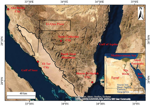
El-Qaa Plain is situated in the South-Western part of Sinai, as shown in Figure 2. It spans between latitudes 27°44’ to 28°54’ North and longitudes 33°12’ to 34°15’ East. This area is a section of the Suez rift margin and stretches along the Gulf of Suez coastline, spanning approximately 95 km in length and 20–30 km in width. It is bordered by the Gebel Qabeliat area to the North-West and the South Sinai Mountains to the East. The major city of El-Tor is located within the El-Qaa Plain, along with Bedouin communities and agricultural settlements. The total area of El-Qaa is approximately 1930 km² (Bakr & El-Beheiry, 2004). Several catchments drain into El-Qaa Plain, encompassing a total catchment area of around 3900 km² (Bakr & El-Beheiry, 2004).

Figure 2. Location of El-Qaa Plain.

Morphology

The topography of the El-Qaa area exhibits a range of slopes, from gentle near the coastline to steep slopes within the mountains (Abuzied & Alrefaee, 2017). The elevation in the area varies from approximately 0 meters to over 2500 meters above Mean Sea Level (MSL), as shown in Figure 3(A). The relief of the study area encompasses low-lying areas as well as high-rugged terrain (Abuzied & Alrefaee, 2017). In the plain region, the surface slope ranges from less than 1% to around 5%, while in the mountainous regions, it varies from around 5% to over 100% (Figure 3(B)).

Figure 3. Morophology of the study area. (A) Elevation. (B) Slope. (C) Land-use. (D) Soil cover.

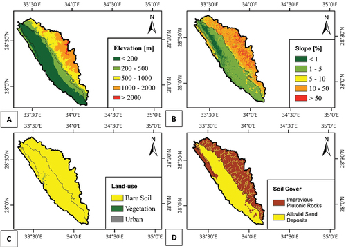
The land-use in the El-Qaa area consists of urban areas, vegetation, and bare soil, as depicted in Figure 3(C). Bare soil covers approximately 99.5% of the total area. Regarding soil cover, Figure 3(D) illustrates the presence of various soil types, including quaternary granular soil, Sabkha deposits (alluvial sand deposits), impervious basaltic soil, pyroclastic soil, and gneiss rocks (impervious rocks). Alluvial sand deposits account for approximately 49% of the total area.

Hydrology

El-Qaa Plain receives water from catchments that drain from the high mountains surrounding it, as shown in Figure 4. These catchments can be categorized into two groups: main catchments, which have an area greater than 10 km², and sub-catchments, which have an area smaller than 10 km². The main catchments in the area include El-Aawag, Isla, El-Mahash, Thoman, El-Raboud, Taalby, Rowais, Abu Markh, Aat El-Gharby, Imaha, and Eghshy (Elewa & Qaddah, 2011; Sherif, 2008).

Figure 4. Catchments draining to El-Qaa Plain (Number of Catchments = 31).

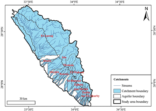
Among these catchments, El-Aawag is the largest catchment in the study area, covering an area of approximately 1920 km². It has the longest stream length of around 71 km and a mean slope of 19%. The mean slope of most catchments ranges from approximately 2% to 24%, while the longest stream length varies from nearly 7 km to 71 km.

Climate

The study area experiences an arid climate, characterized by hot and dry summer days and cold winters with low-intensity precipitation (Abuzied & Alrefaee, 2017). Four meteorological stations are located near the study area: El-Tor, Sharm El-Sheikh, Saint Catherine, and Abo Redies. During summer, the mean temperature is higher than 25°C, while in winter, it is less than 10°C. The annual precipitation in the study area is typically less than 80 mm (Abuzied & Alrefaee, 2017). The mean annual precipitation rate in the study area varies from around 7 mm in El-Tor to 24 mm in Saint Catherine. In the winter season, the mean temperature ranges from approximately 7°C in Saint Catherine to 17°C in Sharm El-Sheikh. During summer, the mean temperature varies from around 25°C in Saint Catherine to approximately 32°C in Sharm El-Sheikh.

Methods

Method selection

Selecting the appropriate method for estimating the recharge depends on different factors including the data availability, feasibility of conducting field measurements and site conditions. Therefore, a thorough literature review was implemented to select the appropriate recharge estimation method based on the aforementioned conditions. Table 1 illustrates the different methods used for estimating the recharge. The table shows the numerical modeling that was chosen to be applied in this study, where many different free numerical models could be applied to estimate the groundwater recharge.

Table 1. List of the applied methods to estimate the mean annual recharge rate by the previous researchers.

Method	Applicability in this study	Reason
Lysimeter method	Not-applicable	Very expensive method
Seepage meter method	Not-applicable	Absence of perennial streams and irrigation channels
Empirical methods	Not-applicable	Doesn’t consider the spatial variability
Zero flux plane method	Not-applicable	Lack of soil moisture parameters data
Estimation of unsaturated zone fluxes	Not-applicable	Lack of soil moisture parameters data
Estimation of saturated fluxes	Not-applicable	Uncertainty of calculating the sink flow to sea and change in storage
Soil moisture budget	Not-applicable	Lack of soil moisture variables data
Watershed budget	Not-Applicable	Lack of flow hydrograph data
Groundwater table fluctuations (aquifer budget)	Not-applicable	Observed groundwater levels in the study area are characterized by low fluctuations
Numerical modeling	Applicable	Can estimate the recharge under limited data availability
Tracer method	Not-applicable	Research potentiality

After conducting a thorough literature review on various numerical models, the Water and Energy Transfer between Soil, Plants, and Atmosphere under quasi-Steady State (WetSpass) model, developed by Batelaan and De Smedt (2001), was selected for estimating the groundwater recharge in this study. The WetSpass model was chosen due to its ability to utilize long-term climate data, topography, land-use information, and soil cover to estimate the spatial distribution of average recharge. By considering these factors, the WetSpass model is expected to provide valuable insights into the groundwater recharge dynamics in the study area.

Data acquisition

Prior to building the WetSpass model, various data sets were acquired to incorporate important factors such as climate, elevation, land-use, and soil cover. Here are the details of the data acquisition process:

• Elevation: Elevation data was processed using ArcGIS 10.7.1 software. The Shuttle Radar Topography Model (SRTM) 90 m Digital Elevation Model (DEM) was obtained from a website of NASA (National Aeronautics and Space Adminstration) (2018). This data source provides detailed elevation information for the study area.

• Surface Slope: The surface slope was calculated using ArcGIS 10.7.1 software based on the acquired elevation data.

• Land-Use Classification: The land-use classification was obtained by processing a Landsat 7 image. Unsupervised image processing techniques were applied using ArcGIS 10.7.1 software. The Landsat 7 image was obtained from USGS (2019).

• Soil Cover: The soil cover data was acquired by digitizing the hydrogeological map of South Sinai created by JICA (Japan International Cooperation Agency) (1999b). This process was performed using ArcGIS 10.7.1 software.

• Climate Data: Climate data was collected from different sources such as WRRI (Water Resources Research Institute) (2016) and UNESCO Cairo office (2005). The nearby meteorological stations, namely Sharm El-Sheikh, El-Tor, Saint Catherine, and Abo-Redies, were chosen to obtain the climate data. The data covers the period from 1986 to 2015 on a monthly basis. The required climate variables for this study include precipitation, maximum temperature, minimum temperature, and surface wind speed.

Data processing

Estimating the potential evapotranspiration

Due to the lack of potential evapotranspiration measurements in the study area, the potential evapotranspiration was estimated using the Hargreaves method. This method was chosen for the following reasons:

• Simple Calculation: The Hargreaves method involves a straightforward calculation that requires only temperature data (maximum and minimum). It does not require additional data related to heat storage of soil, crops, or net solar radiation.

• Applicability in Arid and Semi-Arid Regions: The Hargreaves method has been successfully applied in arid and semi-arid regions. Studies conducted by Di Stefano and Ferro (1997) in Sicily Island, Southern Italy, Vanderlinden, Giraldez, and Meirvenne (2004) in Southern Spain, and El Afandi and Abdrabbo (2015) in the Nile Delta, Egypt, have demonstrated its accuracy in estimating potential evapotranspiration using this method.

Hence, Hargreaves equation, as modified by Hargreaves and Samani (1985), is used to estimate potential evapotranspiration as shown in Equation 1(1) $\mathit{E}{T}_p=\left(\mathit{KT}\right)\left(R_a\right)(\mathit{TD}{)}^{0.5}\left(\mathit{TC}+17.8\right)$(1) .

(1) $\mathit{E}{T}_p=\left(\mathit{KT}\right)\left(R_a\right)(\mathit{TD}{)}^{0.5}\left(\mathit{TC}+17.8\right)$(1)

where $\mathit{E}{T}_p$ is the potential evapotranspiration (mm/day). $R_a$ is the extraterrestrial radiation depending on the latitude (mm/day), TD is the difference between the maximum temperature and the minimum temperature (^oC), TC is the average temperature (^oC). KT is the empirical coefficient (-), ranges from around 0.16 to 0.25 depending on the location (interior regions and coastal regions).

In this study, specific KT values were assigned based on the location of the meteorological gauges. For coastal meteorological gauges, a KT value of 0.21 was assigned, while for inland meteorological gauges, a KT value of 0.16 was assigned. These values were adjusted based on measurement data obtained from a nearby meteorological gauge in Hurghada, which is located near the study area. The measurement data was provided by the Food and Agriculture Organization (FAO) organization.

Interpolating the climate data

To provide spatially distributed climate data for the WetSpass model, interpolation techniques are utilized. In this study, the Inverse Distance Weighting (IDW) method was chosen for climate data interpolation after conducting a thorough literature over the different spatial distribution methods (Table 2). The IDW method is considered an accurate deterministic approach for interpolating climate data and has been verified by Goovaerts (2000), Lu and Wong (2008), Ly, Charles, and Degre (2011), and Chen and Liu (2012).

Table 2. Applicability of the Interpolation techniques.

Spatial distribution method	Applicability	Reason
Uniform distribution (arithmetic average)	Not-applicable	Arid climate is characterized by high spatial and temporal variation especially precipitation.
Kriging weights (Isohetytal contours)	Not-applicable	The number of gauges is small such that variogram analysis is difficult to be applied.
The nearest station (Theissen polygon method)	Not-applicable	Arid climate is characterized by high spatial and temporal variation especially precipitation.
Inverse distance weighting (Reciprocal weighting method)	Applicable	Representing the spatial variability considering the distance from the points

The IDW method can be determined using Equation 2(2) $\hat{P}\left(\mathit{x}\right)=\sum _{\mathit{i}=1}^N{\lambda }_i\mathit{P}\left(x_i\right)$(2) , Equation 3(3) ${\sum }_{i=1}^N{\lambda }_i=1$(3) , and Equation 4(4) ${\lambda }_i=\frac{1/{d_i}^{\mathit{\alpha }}}{{\sum }_{i=1}^N\left(1/{d_i}^{\mathit{\alpha }}\right)}$(4) as mentioned by Chin (2013). By applying the IDW interpolation technique, the available climate point data can be spatially distributed across the study area, providing a climate dataset for the WetSpass model.

(2) $\hat{P}\left(\mathit{x}\right)=\sum _{\mathit{i}=1}^N{\lambda }_i\mathit{P}\left(x_i\right)$(2)

where $\hat{P}\left(\mathit{x}\right)$ is the interpolated rainfall at location x. $\mathit{P}\left(x_i\right)$ is the measured precipitation at rain gauge $\mathit{i}$ that is located at $x_i$, ${\lambda }_i$ is the weight given to measurements at station i, and these weights generally satisfy the relation as shown in Equation 3(3) ${\sum }_{i=1}^N{\lambda }_i=1$(3) .

(3) ${\sum }_{i=1}^N{\lambda }_i=1$(3)

The weight assigned to each is inversely proportional to the distance from the estimation point to the measurement station. This relation is first introduced by Wei (1973) and Simanton and Osborn (1980) as shown in Equation 4(4) ${\lambda }_i=\frac{1/{d_i}^{\mathit{\alpha }}}{{\sum }_{i=1}^N\left(1/{d_i}^{\mathit{\alpha }}\right)}$(4) .

(4) ${\lambda }_i=\frac{1/{d_i}^{\mathit{\alpha }}}{{\sum }_{i=1}^N\left(1/{d_i}^{\mathit{\alpha }}\right)}$(4)

where $d_i$ is the distance to station $\mathit{i}$, and N is the number of stations within some defined radius of where rainfall is to be estimated, $\mathit{\alpha }$ is a power parameter which ranges from 0 to 5. According to Stow (1998), $\mathit{\alpha }$ is set to 2 for the monthly time steps, 3 for the hourly time step, and 1 for the yearly time step. Additionally, Goovaerts (2000) proved that the best value for is 2. Consequently, a power value of 2 was adopted for this study. A python script was written to interpolate the rainfall gauges for all the stations using the inverse distance weighting method.

Numerical modeling

Model description

The WetSpass model (Water and Energy Transfer between Soil, Plants, and Atmosphere under quasi-steady State) is a quasi-steady-state model that is used to estimate the long-term mean recharge rate, taking into account various factors such as spatial distribution, soil texture, land-use, topography, and climate. This model was developed by Batelaan and De Smedt (2001).

The WetSpass model is a grid distributed model, where a mass balance is applied to each grid cell individually rather than considering the mass balance for the entire system. Equation 5(5) $\mathit{R}=\mathit{P}-\mathit{ET}-\mathit{S}-\mathit{I}$(5) represents the main governing equation of the WetSpass model, as described by Batelaan and De Smedt (2001).

By incorporating spatial distribution, soil texture, land-use, topography, and climate factors, the WetSpass model provides a comprehensive approach to estimating recharge rates in a quasi-steady-state. This allows for a better understanding of the groundwater recharge process and its variations across the study area.

(5) $\mathit{R}=\mathit{P}-\mathit{ET}-\mathit{S}-\mathit{I}$(5)

where $\mathit{P}$ is the monthly precipitation (L/T), $\mathit{I}$ is the monthly interception (L/T),$\mathit{ET}$ is the monthly actual evapotranspiration(L/T), $\mathit{S}$ is the monthly runoff (L/T), and $\mathit{R}$ is the monthly recharge (L/T).

The hydrological variables are calculated based on the change in land-use type at a certain grid as shown in Equation 6(6) $\mathit{E}{T}_{\mathit{grid}}=a_v\mathit{E}{T}_v+a_s\mathit{E}{T}_s+a_o\mathit{E}{T}_o+a_i\mathit{E}{T}_i$(6) ), Equation 7(7) $S_{\mathit{grid}}=a_v{S}_v+a_s{S}_s+a_o{S}_o+a_i{S}_i$(7) ), and Equation 8(8) $R_{\mathit{grid}}=a_v{R}_v+a_s{R}_s+a_o{R}_o+a_i{R}_i$(8) .

(6) $\mathit{E}{T}_{\mathit{grid}}=a_v\mathit{E}{T}_v+a_s\mathit{E}{T}_s+a_o\mathit{E}{T}_o+a_i\mathit{E}{T}_i$(6)

(7) $S_{\mathit{grid}}=a_v{S}_v+a_s{S}_s+a_o{S}_o+a_i{S}_i$(7)

(8) $R_{\mathit{grid}}=a_v{R}_v+a_s{R}_s+a_o{R}_o+a_i{R}_i$(8)

where $\mathit{E}{T}_{\mathit{grid}}$, $S_{\mathit{grid}}$, $R_{\mathit{grid}}$ are respectively the actual evapotranspiration, surface runoff, and groundwater recharge of a grid cell, (L), and $a_v$, $a_s$, $a_o$, $a_i$ are respectively a fraction area of vegetation, bare-soil, open-water and impervious area.

Interception is calculated in the model as a ratio of precipitation. This ratio depends on land use and soil texture type (Abdollahi, 2015). Equation 9(9) $\mathit{I}=\mathit{P}\left(1-e^{\left(\frac{-I_D{d}_p}{\mathit{P}}\right)}\right)$(9) shows the interception calculation as described by (Abdollahi, 2015).

(9) $\mathit{I}=\mathit{P}\left(1-e^{\left(\frac{-I_D{d}_p}{\mathit{P}}\right)}\right)$(9)

where I is the monthly interception (L/T), P is the monthly precipitation (L/T), $d_p$ is the number of rainy days per month (-) and $I_D$ is the daily interception threshold (depends on land-use) (-).

Surface runoff is calculated in the model based on the rational method applied on a monthly time step via Equation 10(10) $\mathit{S}=C_{\mathit{sr}}{C}_h\left(\mathit{P}-\mathit{I}\right)$(10) as described by Abdollahi (2015).

(10) $\mathit{S}=C_{\mathit{sr}}{C}_h\left(\mathit{P}-\mathit{I}\right)$(10)

where S is the monthly runoff (L/T), $C_{\mathit{sr}}$ is the actual runoff coefficient (-),$C_h$ is a coefficient that depends on soil moisture condition (-).

Evapotranspiration is calculated per grid by adding the actual evapotranspiration of the vegetated, open water, bare soil, and impervious land-use classes. To calculate the actual evapotranspiration ($\mathit{ET}$), a vegetation coefficient (c) is required as shown in Equation 11(11) $\mathit{ET}=\mathit{cE}{T}_p$(11) as mentioned by Abdollahi (2015).

(11) $\mathit{ET}=\mathit{cE}{T}_p$(11)

Where c is a vegetation coefficient, $\mathit{ET}$ is the actual evapotranspiration, $\mathit{E}{T}_p$ is the potential evapotranspiration.

Setting-up the model

In order to setup WetSpass model, the acquired data were imported to the model. However, the data were processed before importing. As the geomorphological data and climate data were converted to the ASCII file format. The grid size for the ASCII files was discretized to 250 meters.

There are two types of input raster data that need to be imported into WetSpass:

• Spatially Distributed Raster ASCII Files: These include elevation, land-use, soil cover, and surface slope data. Each of these datasets is represented in the ASCII file format with a spatial distribution of 250 meters.

• Spatially and Temporally Distributed Raster ASCII Files: These include precipitation, potential evapotranspiration, surface wind speed, and mean temperature data. These datasets are also represented in the ASCII file format with a spatial distribution of 250 meters. However, in addition to the spatial distribution, these files also capture the temporal distribution on a monthly basis. This allows the model to consider the variability of these climate variables over time.

Calibrating the model

In a research study conducted by Melki, Abdollahi, Fatahi, and Abida (2017) in the Northern Gafsa watershed, Tunisia, the impact of precipitation on natural groundwater recharge was investigated. The WetSpass model was calibrated based on an agreement between the runoff and recharge values obtained from the model and the difference between rainfall and potential evapotranspiration values obtained from 50-year measurements.

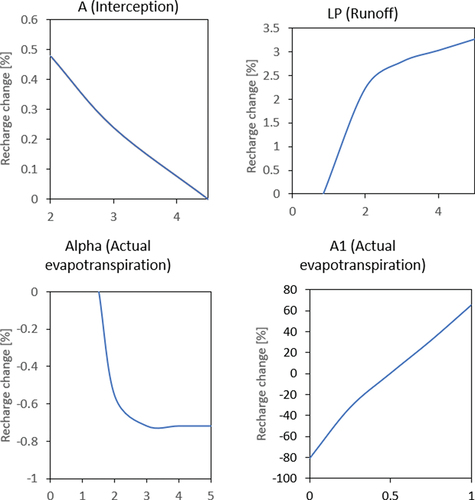
Melki, Abdollahi, Fatahi, and Abida (2017) identified four main parameters that significantly affect the model results (sensitive parameters): a (coefficient related to interception equation), alpha (coefficient related to actual evapotranspiration equation), LP (coefficient related to runoff equation), and A1 (coefficient related to actual evapotranspiration equation). Therefore, in our case study, these four main sensitive parameters determined by Melki, Abdollahi, Fatahi, and Abida (2017) were considered for the calibration process.

Prior to calibrating the model, sensitivity analysis was performed for the determined sensitive model parameters (Figure 5). The analysis results demonstrate that A1 is considered the most sensitive parameter, as it significantly alters recharge by around 80%. Additionally, it has been perceived that alpha and LP coefficient are more sensitive at lower ranges respectively: (1.5 - 2.5), (0.85 - 2). Moreover, recharge is slightly sensitive to a and alpha, as the relative change value always maintains below 1% within the whole range of both parameter.

Figure 5. Model Sensitivity Analysis.

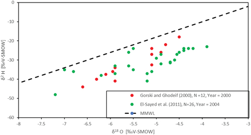
The model was calibrated by analyzing the isotope signature enrichment. According to Clarke and Fritz (1997), rainfall isotopes become enriched due to evaporation processes in arid and semi-arid regions. Therefore, this method is appropriate for estimating the recharge in case that the main source of the groundwater is just the rainfall. Allision, Barnes, Hughes, and Leaney (1984) found that shift of the isotope delta from the Local Meteoric Water Line (LMWL) is inversely proportional to the square root of the annual groundwater recharge. Clarke & Fritz (1997) have formulated this relation as shown in Equation 12.(12) ${\delta }^2{H}_{\mathit{shift}}=\frac{1}{\mathit{GW}{\mathit{R}}^{0.5}}$(12)

(12) ${\delta }^2{H}_{\mathit{shift}}=\frac{1}{\mathit{GW}{\mathit{R}}^{0.5}}$(12)

where δ2 H_shift is the groundwater deuterium shift from LMWL, and GWR is the annual mean groundwater recharge.

The significant recharge of the aquifer system is originated from the new continental and mediterranean rains and precipitated water from dominant wet climate periods with seldom contribution of fossil groundwater as deduced by. Thus, the aforementioned equation could be applied to calculate the mean annual recharge rate. To implement that, isotope signature data were acquired from previous studies for the year 2000 and 2004 respectively: Gorski and Ghodeif (2000), El-Sayed, Sabet, and Ali (2011). Figure 6 shows the plot of the relationship between δ18O and δ2H, where the collected data were plotted along with the Mediterranean Meteoric Water Line (MMWL). MMWL has resembled the LMWL in this region as it was proved by Elewa et al. (2023).

Figure 6. Environmental stable isotopes composition (δ¹⁸O and δ²H) of groundwater samples.

To execute the mean annual recharge rate for both datasets, the deuterium shift was identified by subtracting the deuterium isotope signature of groundwater sample from that of MMWL. Afterwards, the mean annual recharge rate was calculated for both datasets by averaging the mean value of each sample. The calculated value is then used to calibrate the model. Table 3 mentions the values of the adjusted calibrated parameters, whereas Table 4 evaluates the performance of the calibration process.

Table 3. Calibrated parameter values.

Parameter	Equation type	Parameter range assigned by the model developer	Calibrated parameters
A	Interception equation	2 - 4.5	2
Alpha	Evapotranspiration equation	1.5 - 5	1.5
LP	Runoff equation	0.85 - 5	5
A1 (sand)	Evapotranspiration equation	0 - 1	1.0
A1 (Clay)	Evapotranspiration equation	0 - 1	0.4

Table 4. Model calibration performance evaluation.

Dataset	Year	Mean annual recharge rate (isotope) [mm/year]	Mean annual recharge rate (model) [mm/year]	Relative change [%]
Gorski and Ghodeif (2000)	2000	4.15	4.17	0.48
El-Sayed, Sabet, and Ali (2011)	2004	3.99	4.05	1.48

Running the model

After calibrating the WetSpass model, the model was run for a period of 30 years, from 1985 to 2015, with a monthly time step. The successful completion of the model run provided the required outputs for further analysis. To facilitate the visualization and interpretation of the results, Python scripts were prepared. These scripts allow for the graphical representation of the inter-annual variability and seasonal variability of recharge, as well as the quantification of important hydrological variables such as precipitation, runoff, and actual evapotranspiration.

Furthermore, maps were generated to depict the spatial variability of the different hydrological components and their relationship with various factors: topography, soil cover, land-use. These maps help to understand how these factors influence the distribution and behavior of the hydrological variables across the study area. To specify the annual volume range of the hydrological range, a symmetric confidence interval was calculated using the student's t distribution with a confidence level of 95%. With 30 years of data, the t-value is 2.064.

Validating the model results

The MODFLOW model was utilized to validate the recharge results obtained from the WetSpass model. Soliman, Hafiz, Amin, and Bekhit (2022) set up, calibrated, and validated the MODFLOW model using various input data. This included providing the top and bottom elevations of the aquifer, defining sources and sinks, specifying boundary conditions, and determining hydraulic conductivity and specific yield.

To calibrate the MODFLOW model, the hydraulic conductivity parameter was adjusted to match the observed groundwater level contour lines, ensuring a good fit between the model predictions and the actual measurements.

Subsequently, the model was run under the transient state condition from the year 2000 until 2011 using the recharge data generated by the WetSpass model. This period was selected due to the availability of groundwater level measurement data for the study area during this period. The specific yield was set to 0.25 as assumed by Zaghlool and Eissa (2018), while the storativity parameter was estimated as 0.00015. The determination of the storativity paramter involved multiplying the average saturated thickness of the aquifer by a factor of 10⁻⁶, as stated by Todd and Larry (2004).

The recharge values generated by the WetSpass model were incorporated into the MODFLOW model for the period from 2000 to 2011. The MODFLOW model simulated the groundwater levels, which were then compared to the observed groundwater level time series.

The comparison between the observed and simulated groundwater levels revealed a good agreement, as demonstrated in Figure 6, Figure 7, and Table 5. The Mean Absolute Error (MAE) and Root Mean Square Error (RMSE) were both below 0.5 and 0.6 m, respectively, for most of the observation wells. However, it should be noted that Peizometer 8 exhibited larger errors, primarily due to the presence of outlier records in the observed groundwater level time series.

Figure 7. Validating the WetSpass resutls using MODFLOW model by comparing the simulated groundwater level with the measured leved for the period (2000 – 2011).

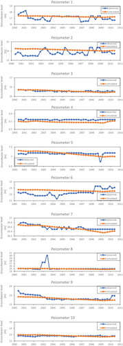
Table 5. Model validation performance evaluation using Mean Absolute Error (MAE) and Root Mean Square Error (RMSE) goodness of fit.

Piezometer	1	2	3	4	5	6	7	8	9	10
MAE [m]	0.35	0.39	0.07	0.06	0.10	0.59	0.07	0.34	0.16	0.12
RMSE [m]	0.44	0.44	0.08	0.06	0.12	0.65	0.08	0.95	0.21	0.14

Overall, the results indicate that the recharge values obtained from the WetSpass model yield reasonable and reliable results when applied in the MODFLOW model. The model’s ability to accurately simulate the groundwater levels, as proved by the performance evaluation indicators, further supports the validity of the recharge estimates obtained from the WetSpass model.

Results and discussion

Temporal variability of recharge

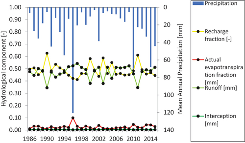
Figure 8 depcits the inter-annual variability of various hydrological variables: recharge, actual evapotranspiration, runoff, interception. The cumulative annual precipitation values are represented by inverted blue bars, while the other hydrological variables are presented as scatter points, represented as a fraction of the precipitation. The inter-annual variability of the hydrological variables can provide valuable information about the water balance and dynamics within the study area. It aids to understand the relationships and interactions between these variables, hence understanding the entire hydrological system in the study area.

Figure 8. Inter-annual variability of the hydrological components fraction.

Table 6 provides an overview of the statistical properties of these hydrological components in relation to the precipitation. It includes various statistical measures such as the mean, standard deviation, minimum, and maximum values. These statistics reflects the variability, distribution, and characteristics of the hydrological variables relative to the precipitation values.

Table 6. Statistical properties of the hydrological components fraction.

Statistical property	Precipitation [mm]	Recharge fraction [-]	Actual evapotranspiration fraction [-]	Runoff fraction [-]	Interception fraction [-]
Mean	26.389	0.471	0.041	0.483	0.003
Median	18.134	0.455	0.022	0.450	0.003
Max	120.699	0.626	0.100	0.543	0.006
Min	2.921	0.411	0.010	0.344	0.002
Standard deviation	25.99	0.05	0.02	0.05	0.001

From the results presented in Figure 8, it can be observed that the recharge fraction ranges from approximately 0.41 to 0.63 (Table 6). The interception coefficient remains relatively constant at around 0.003. The actual evapotranspiration fraction shows slight variations, ranging from about 0.01 to 0.1. The runoff fraction is significantly influenced by precipitation, with wet years exhibiting higher runoff fractions (e.g., around 0.54 in 1996) and dry years showing lower runoff (nearly 0.34). High recharge fractions (>0.55) are observed in certain years (e.g., 1990, 1992, 2000, 2003, 2005, 2011) when cumulative annual precipitation ranges from approximately 5 mm to 10 mm except year 2011. Thus, it has been predicted that a significant portion of precipitation is stored in the soil after interception and evapotranspiration processes, leading to lower runoff discharge. When precipitation exceeds approximately 10 mm, the soil becomes saturated, resulting in increased runoff generation and subsequently higher runoff fractions. However, the actual evapotranspiration remains relatively constant in this precipitation range.

In Figure 9, the relationship between the different hydrological variables is plotted, considering the seasonal variability. It is evident that the summer season (June, July, August) experiences no precipitation events, indicating a seasonal hydrological system where the streams are ephemeral. Precipitation remains relatively constant in other months, with mean monthly precipitation ranging from 1.5 to 2 mm, except in January when it reaches around 3.5 mm. April, May, and September exhibit very low mean monthly precipitation, ranging from 0 to 0.2 mm.

Figure 9. Inter-annual variability of the hydrological components fraction.

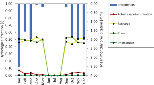
The analysis of seasonal variability reveals that most precipitation is allocated to runoff and recharge flow components, with the recharge fraction ranging from 0.43 to 0.53 and runoff fraction ranging from 0.45 to 0.54. The winter season (December, January, February) exhibits slightly higher actual evapotranspiration fractions (reaching around 0.07 in January). High actual evapotranspiration is expected in Winter due to the availability of water in the vadose zone. The interception fraction remains relatively constant at 0.003, except during the summer season, where it vanishes.

Spatial variability of hydrological components

From the spatial variability analysis shown in Figure 10, several key observations can be distinguished regarding the different hydrological variables. Regarding recharge (Figure 10(A)), it is evident that the recharge fraction is significantly influenced by the soil cover. In areas where impervious plutonic rocks are present, such as the high mountains, the recharge fraction is low (< 0.1) except at the ephemeral streams, where water infiltrates to the vadose zone and then percolates to the groundwater. Conversely, in areas with alluvial sand deposits, such as the plain, high recharge is expected (> 0.5).

Figure 10. Spatial variability of different hydrological variables. (A) Recharge. (B) Actual Evapotranspiration. (C) Runoff. (D) Interception.

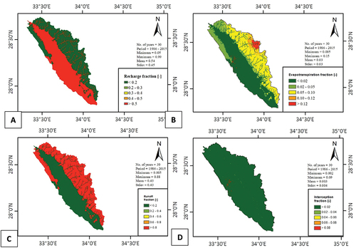
The spatial variability of actual evapotranspiration (Figure 10(B)) is affected by both soil cover, land-use and the spatial variability of precipitation. The map indicates that actual evapotranspiration is generally high at the high mountainous areas (>0.05). However, in agricultural areas, the actual evapotranspiration coefficient ranges from approximately 0.3 to 0.4. Nevertheless, in urban areas and bare soil areas, it maintains below 0.02.

The distribution of runoff (Figure 10(C)) is mainly influenced by the slope and the soil type. High mountainous regions tend to exhibit higher runoff exceeding 0.8. The topography of the system also plays a role, with steep slopes (50-100%) associated with higher runoff, while areas with gentle slopes (1-5%) show lower runoff. Land-use also influences runoff, with higher runoff fractions (> 0.8) observed in urban areas, where impervious surfaces and limited soil storage are present. In contrast, the interception fraction is significantly influenced by the vegetation situated at the agricultural areas exhibiting higher interception fractions (> 0.06), and it diminishes in the latter areas (Figure 10(D)).

Specfying the annual recharge rate

The analysis of the mean annual recharge rate over the period of 1986-2015 reveals that the average recharge rate is approximately 12.36 mm/year. To determine the range of the annual recharge rate. The calculated 95% confidence interval ranges from around 8.10 mm/year to 16.62 mm/year. The mean recharge coefficient, which represents the ratio of recharge to precipitation, is approximately 0.47. The 95% confidence interval for the recharge coefficient ranges from 0.45 to 0.49.

Furthermore, the mean volume of the main hydrological components (recharge, runoff) were calculated along with their 95% confidence intervals (Table 7) The mean annual recharge volume ranges from approximately 16 Mm³ to 32 Mm³, while the mean annual runoff volume ranges from 15 Mm³ to around 34 Mm³.

Table 7. Statistical properties of the annual volume of the different hydrological components (period: 1985 – 2015).

Statistical property	Annual precipitation volume (Mm^3/year)	Annual recharge volume (Mm^3/year)	Annual actual evapotranspiration volume (Mm^3/year)	Annual runoff volume (Mm^3/year)	Annual interception volume (Mm^3/year)
Mean	50.93	23.97	2.08	24.59	0.15
Median	36.71	16.69	0.81	16.54	0.13
Max	232.95	98.01	23.31	121.88	0.37
Min	5.64	2.76	0.06	2.71	0.03
95% Confidence interval (-ve)	13.34	6.28	0.54	6.44	0.04
95% Confidence interval (+ve)	32.23	15.71	0.47	15.12	0.12

The generated map (Figure 11) provides the spatial variability of the mean annual recharge rate across the study area. The map shows different zones with varying recharge values. Low recharge values (less than 4 mm/year) are observed in the high mountains (impervious plutonic rocks cover), and urban areas such as El-Tor city. These areas exhibit limited recharge potential due to geological and landuse characteristics of impervious and semi-impervious surfaces.

Figure 11. Recharge distribution map.

Moderate recharge values (ranging from more than 4 mm/year to less than 8 mm/year) are predominantly found in the agricultural areas characterized by presence of crop vegetation and gentle slope. High recharge values (varying from more than 8 mm/year to less than 12 mm/year) could be located at the bare areas, where just sparse vegetation is situated. These regions have relatively better recharge potential compared to the aforementioned zones. High recharge values (greater than 12 mm/year) are primarily located in the streams present in the high mountainous areas. These streams act as pathways for water to flow into the aquifer, resulting in higher recharge rates.

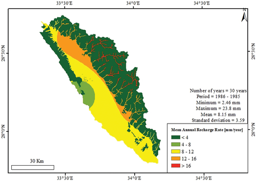
The statistical analysis of the recharge spatial variability indicates that the dispersion of recharge values from the mean is relatively small, with a maximum deviation of 4 mm. The highest recharge value observed in the mountainous streams is approximately 23.8 mm/year, while the lowest value of 2.46 mm/year is recorded in a mountainous area characterized by impervious rock soil cover. These findings highlight the spatial heterogeneity of recharge rates within the study area. They emphasize the influence of geological features, soil cover, and land topography on groundwater replenishment. This information can be valuable for understanding the water balance of the system and informing sustainable water management practices.

Discussion

The study highlights the accuracy and precision of estimating the recharge rate conducted using the WetSpass model. By considering various factors such as land use, soil cover, slope, and precipitation, the model provides reliable estimates of recharge on a long-term basis, incorporating temporal and spatial variability.

Overall, the inter-annual variability highlights the strong influence of runoff and precipitation hydrological components on recharge, as the recharge fraction is inversely proportional to both precipitation and runoff fractions. On the other hand, the actual evapotranspiration is only slightly affected by precipitation (direct relationship), while the interception coefficient is not influenced by precipitation due to lack of presence of canopy surfaces in the study area except at the agricultural areas.

The results demonstrate that land use plays a crucial role in determining recharge rates. Impervious areas at the high mountains exhibit high actual evapotranspiration and high runoff coefficients resulting in extremely low recharge rates. Bare soil at permeable areas has relatively low actual evapotranspiration and low interception due to presence of less dense sparse vegetation, and low runoff coefficients (gentle slopes) causing high recharge rates. Also, agricultural areas are characterized by high interception and actual evapotranspiration leading to lower recharge rates.

Soil texture is another important factor influencing the recharge fraction. Sandy soil areas exhibit higher recharge coefficients compared to areas with impervious plutonic rocks. Additionally, slope significantly affects the runoff coefficient and recharge rates such that low slope areas are characterized by lower runoff and vice versa.

Precipitation is the main driver of the hydrological system and strongly influences recharge. High precipitation events lead to increased runoff and actual evapotranspiration volumes, causing a decrease in recharge. Conversely, low precipitation events lead to minimal runoff and increased recharge volumes.

Comparing the mean annual recharge rate with previous studies, it has been inferred that the mean annual recharge rate obtained in this study aligns closely with the estimated mean annual recharge rate calculated by USAID (1986) and Tamaam (2012). As they estimated the values using the SCS-CN loss and transform method. On the other hand, it might be deduced that the recharge rate in this study is overestimated if it is compared to the estimated values by the latter studies.

Comparing the recharge fraction with the studies around the globe, the recharge in this study might be overestimated (0.47) if it is compared to the rule of thumb claimed by Jyrkama and Sykes (2007). As they stated that the recharge rate in most regions of the world is around 0.33. Nevertheless, the recharge fraction in arid climate regions is expected to be high due to the following reasons: difficulty of soil saturation due to soil characteristics and climate conditions enabling for high recharge rates during precipitation events, low dense sparse vegetation causing reduction of evapotranspiration and interception components, no presence of organic matter in the soil, no presence of base-flow in the system.

The recharge fraction specified from this study approaches the fractions calculated by some researchers at different regions characterized by arid climate environment: Marei et al. (2010) for West Bank, Palestine (0.15 – 0.5), Githui, Selle, and Thayalakumaran (2012) for Southeast Australia (0.4). Yet, the recharge fraction highly relies on the study area characteristics such as topography, soil cover and landuse.

Despite of the capability of Wetspass to estimating the recharge precisely; as it considers the spatial distribution of landuse, soil cover, topography and climate, limitations take place. Firstly, the model can’t be run at smaller time step leading to over-estimated or under-estimated recharge values in case of extreme rainfall events with certain distribution pattern. Secondly, the model grid are not connected together via a flow network. This might cause inaccuracy of estimating the recharge especially if the base flow hydrological component is active in the study area. Finally, the model is based on multiple assumptions that simplifies the hydrological process. If the user lacks experience using this model, he may interpret wrong results.

The mean annual recharge rate might be employed to calibrate groundwater flow models, particularly for determining hydraulic conductivity through inverse groundwater modeling. The precise calculation of the mean annual recharge rate, considering spatial and temporal variability, enhances the accuracy of groundwater flow models. Additionally, the groundwater flow modelers could benefit from the results by importing the annual recharge rate to the groundwater flow model. As they could simulate different groundwater exploitation scenarios to propose groundwater management plans.

Although the current groundwater recharge has been estimated, the groundwater recharge might be altered in the future as a consequence of climate change and change of landuse. As plenty of studies have investigated the link between the climate change and groundwater recharge in terms of quantity and time (Döll, 2009), (Green et al., 2011). Whereas, the latter studied the impact of groundwater abstractions and change in landuse under reduced groundwater recharge (Henrique et al., 2011). Thus, estimation of groundwater recharge under climate change, change in landuse has to be analyzed for the study area.

Conclusion

Groundwater recharge estimation was conducted in the El-Qaa Plain Aquifer, located in Sinai, Egypt, using the WetSpass model considering spatial and temporal variability. The analysis of hydrological variables (precipitation, recharge, actual evapotranspiration, runoff) provided better understanding of the hydrological system. The study also determined the mean annual recharge rate with high precision and specified annual recharge range.

The estimated mean annual recharge rate of 12.36 mm/year provides a reliable measure of groundwater replenishment in the study area along with a 95% confidence interval ranging from 8.10 to 16.62 mm/year. The corresponding annual recharge volume ranged from 16 Mm³ to 32 Mm³, while the runoff volume varied from 15 Mm³ to around 34 Mm³. The recharge coefficient (a measure of the proportion of precipitation contributing to recharge) was determined to be between 0.45 and 0.49, indicating the aquifer potential for replenishing the groundwater. These values align well with similar studies conducted in arid regions worldwide, strengthening the credibility to the results.

These findings have important implications for future water resource management, as they suggest the potential construction of dams to store excess runoff and mitigate flash flood events, where more storage dams could be constructed by total storage capacity of proximately 34 Mm³ to store water in case of extreme flash-flood events. Sand storage dams can be constructed to store harvested water in the unconfined aquifer and protect it from evapotranspiration, ensuring its availability during drought periods.

The results of this study lacks both the effect of the climate change and the change of landuse on the natural groundwater recharge. Additionally, the chosen model unpredicts the recharge value at smaller time steps (day) such that it can not simulate the recharge of high intense and low durational precipitation events. Additionally, the model is based on assumptions that simplifies the hydrological process.

Furthermore, it is recommended that future research should focus on studying the impact of climate change and landuse on groundwater recharge and exploring the feasibility of implementing artificial recharge sites and rainfall harvesting techniques to address potential drought scenarios. Additionally, it is important to estimate the recharge rate using another method to cross validate the studies’ results: tracer method, physical method, numerical model using another model. Moreover, groundwater flow models can be developed to assess the sensitivity of the hydrogeological system to natural recharge. Moreover, water allocation models can optimize the conjunctive use of water resources, including stormwater, desalinated water, and groundwater, to ensure sustainable management practices.

The outcomes of this study hold a significant value for decision-makers involved in water resource management in the study area. The precise estimation of mean annual recharge rates, coupled with the delineation of recharge and runoff volumes, can support the sustainable water resource planning and aid the identification of potential artificial recharge sites. The reliable groundwater flow model derived from the accurate recharge calculations provides a valuable tool for groundwater modelers. Furthermore, hydrogeologists can utilize the groundwater recharge map to identify suitable locations for artificial recharge sites before conducting feasibility studies and pilot projects.

In conclusion, this study’s comprehensive analysis of groundwater recharge in the El-Qaa Plain Aquifer using the WetSpass model, considering spatial and temporal variability, yields valuable insights for sustainable water resource management. The robust findings and recommendations provided herein pave the way for informed decision-making, future research, and the development of effective strategies to mitigate water scarcity challenges in the study area.

Acknowledgments

The authors would like to thank the Water Resources Research Institute (WRRI), National Water Research Center (NWRC), Egypt for providing the necessary data to conduct this research.

Disclosure statement

No potential conflict of interest was reported by the author(s).

References

- Abdelrahman, H. (1996). The potential of water resources in El-Qaa plain. PhD Dissertation. Ain Shams University, Cairo, Egypt.
- Abdollahi, K. (2015). Basin scale water balance modelling for variable hydrological regimes and temporal scales. PhD Dissertation, Vrije Universiteit Brussel, Brussels, Belgium.
- Abuzied, S. M., & Alrefaee, H. A. (2017). Mapping of groundwater propspective zones integrating remote sensing, geographic information systems and geophysical techniques in El-Qaa Plain Area. Hydrogeology Journal, 25(7), 2067–2088.
- Ahmadalipour, A., Moradkhani, H., & Demirel, M. (2017a). A comparative assessment of projected meteorological and hydrological droughts: Elucidating the role of temperature. Journal of Hydrology, 553, 785–797.
- Ahmadalipour, A., Moradkhani, H., & Svoboda, M. (2017b). Centennial drought outlook over the CONUS using NASA-NEX downscaled climate ensemble. International Journal of Climatology, 37(5), 2477–2491.
- Ahmed, M., Sauck, W., Sultan, M., Eugene, Y., Soliman, F., & Rashed, M. (2014). Geophysical constraints on the hydrogeologic and structural settings of the gulf of suez rift-related basins: Case study from the El Qaa Plain, Sinai,Egypt. Surveys in Geophysics, 35(2), 415–430.
- Ali, M., & Mubarak, S. (2017). Approaches and methods of quantifying natural groundwater recharge – A review. Asian Journal of Environment & Ecology, 5(1), 1–27.
- Allison, G. B., Barnes, C. J., Hughes, M. W., & Leaney, F. W. J. (1984). Effect of climate and vegetation on oxygen-18 and deuterium profiles in soils. Isotope hydrology conference 1983, IAEA, Vienna, Austria, 105–123.
- Armanuos, A. M., Negm, A., Yoshimura, C., & Valeriano, O. C. (2016). Application of WetSpass model to estimate groundwater recharge variability in the Nile Delta aquifer. Arab J Geosci, 9(10).
- Bakr, M. I., & El-Beheiry, M. (2004). Stochastic analysis of well capture zones in El-Qaa Plain. Arab Water 2004, Second Regional Conference, Cairo, Egypt.
- Batelaan, O., & De Smedt, F.(2001). WetSpass: A flexible, GIS based, distributed recharge methodology for regional groundwater modelling (pp. 11–18). Wallingford, UK: IAHS Publication.
- Chen, F. W., & Liu, C. (2012). Estimation of the spatial rainfall distribution using inverse distance weighting (IDW) in the middle of Taiwan. Paddy and Water Environment, 10(3), 209–222.
- Chin, D.A.(2013). Water-resources engineering. Newyork, USA: Pearson Education.
- Clarke, I., & Fritz, P. (1997) Environmental isotopes in hydrogeology. Newyork, USA: Lewis Publishers.
- Di Stefano, C., & Ferro, V. (1997). Estimation of evapotranspiration by Hargreaves formula and remotely sensed data in semi-arid Mediterranean areas. Journal of Agricultural and Engineering Research, 68(3), 189–199.
- Döll, P. (2009). Vulnerability to the impact of climate change on renewable groundwater resources: a global-scale assessment. Environmental Research Letters, 4(3), 035006.
- EEC (European Economic Council). (1993). Water resources study in Sinai, Technical Report. Cairo, Egypt.
- El Afandi, G., & Abdrabbo, M. (2015). Evaluation of reference evapotranspiration equations under current climate conditions of Egypt. Turkish Journal of Agriculture - Food Science and Technology, 3(10), 819–825.
- Elewa, H. H., Nosair, A. M., Zelenakova, M., Mikita, V., Abdel Moneam, N. A., &, and Ramadan, E. M. (2023). Environmental Sustainability of Water Resources in Coastal Aquifers, Case Study: El-Qaa Plain, South Sinai, Egypt. Water, 15(6), 1118.
- Elewa, H.H., & Qaddah, A.A.(2011). Groundwater potentiality mapping in the Sinai Peninsula, Egypt, using remote sensing and GIS-watershed-based modeling. Hydrogeology Journal, 19(3), 613–628.
- El-sayed, S. A., Sabet, H. S., & Ali, H. M. H. (2011). Appraisal of groundwater in El Tur Area, Southwest Sinai, Egypt. Isotope and Rad Res, 43(3), 605–632.
- Eltarabily, M. G., Abd-Elaty, I., Elbeltagi, A., Zeleňáková, M., & Fathy, I. (2023). Investigating Climate Change Effects on Evapotranspiration and Groundwater Recharge of the Nile Delta Aquifer, Egypt. Water,15(3), 572.
- Eris, E., Cavus, Y., Aksoy, H., Burgan, H. I., Aksu, H., & Boyacioglu, H. (2020). Spatiotemporal analysis of meteorological drought over Kucuk Menderes River Basin in the Aegean Region of Turkey. Theoretical and Applied Climatology, 142(3–4), 1515–1530.
- Fetter, C.W.(2018). Applied hydrogeology. Illinois, USA: Waveland Press.
- Githui, F., Selle, B., & Thayalakumaran, T. (2012). Recharge estimation using remotely sensed evapotranspiration in an irrigated catchment in southeast Australia. Hydrological Processes, 26(9), 1379–1389.
- Goovaerts, P.(2000). Geostatistical approaches for incorporating elevation into the spatial interpolation of rainfall. Journal of Hydrology, 228(1–2), 113–129.
- Gorski, J., & Ghodeif, K. (2000). Salinization of shallow water aquifer in El-Qaa coastal plain, Sinai, Egypt. 16th Salt Water Intrusion Meeting, Miedyzydoje-Wolin Island, Poland.
- Green, T. R., Taniguchi, M., Kooi, H., Gurdak, J. J., Allen, D. M., Hiscock, K. M., Treidel, H., & Aureli, A. (2011). Beneath the surface of global change: Impacts of climate change on groundwater. Journal of Hydrology, 405(3–4), 532–560.
- Hargreaves, G. H., & Samani, Z. A.(1985). Reference crop evapotranspiration from temperature. Applied Engineering Agriculture, 1(2), 96–99.
- Healy, R. W.(2010). Estimating groundwater recharge. London, UK: Cambridge University Press.
- Henrique, M. L., Chaves, A. P. S., Rejane, M. M. (2011). In Treidel, H., Martin-Bordes, J. L., Gurdak, J. J Eds. Climate change effects on groundwater resources: a global synthesis of findings and recommendations. Poca Raton, Florida, USA: CRC Press. Groundwater discharge as affected by landuse change in small catchments: A hydrologic and economic case study in central Brazil.
- Islam, S., Singh, R. K., & Roohul, A. K. (2015). Methods of estimating groundwater recharge. International Journal of Engineering Associates, 5(2), 6–9.
- JICA (Japan International Cooperation Agency) (1999a). South Sinai groundwater resources study in the arab republic of Egypt, Technical Report, El-Qanater El-Khayriya, Egypt.
- JICA (Japan International Cooperation Agency) (1999b). Hydrogeological map of South Sinai, Data. Egypt: El-Qanater El-Khayriya.
- Jyrkama, M. I., & Sykes, J. F. (2007). The impact of climate change on spatially varying groundwater recharge in the grand river watershed (Ontario). Journal of Hydrology, 338(3–4), 237–250.
- Lanen, V. H., & Peters, E. (2000). Definition, effects and assessment of groundwater droughts. J. V. Vogt & F. Somma Eds. Drought and drought mitigation in Europe Dordrecht: Springer. Amsterdam, Netherlands. 49–61.
- Li, Z., Eladly, A. S., Amen, E. M., Salem, A., Hassanien, M. M., Yahya, K.E., & Liang, J. (2024). Spatial–Temporal Water Balance Evaluation in the Nile Valley Upstream of the New Assiut Barrage, Egypt, Using WetSpass-M. Water, 16(4), 543.
- Lu, G. Y., & Wong, D. W. (2008). An adaptive inverse-distance weighting spatial interpolation technique. Computers and Geosciences, 34(9), 1044–1055.
- Ly, S., Charles, C., & Degre, A. (2011). Geostatistical interpolation of daily rainfall at catchment scale : The use of several variogram models in the Ourthe and Ambleve catchments, Belgium. Hydrology and Earth System Sciences, 15(7), 2259–2274.
- Marei A., Khayat S., Weise S., Ghannam S., Sbaih M., & Geyer, S. (2010). Estimating groundwater recharge using the chloride mass-balance method in the West Bank, Palestine. Hydrological Sciences Journal, 55(5), 780–791.
- Melki, A., Abdollahi, K., Fatahi, R., & Abida, H. (2017). Groundwater recharge estimation under semi arid climate: Case of Northern Gafsa watershed, Tunisia. Journal of African Earth Sciences, 132, 37–46.
- MWRI (Ministry of Water Resources and Irrigation). (2024). water (in arabic). Accessed 25 4, 2024. https://www.mwri.gov.eg/water.
- NASA (National Aeronautics and Space Adminstration) (2018). Digital elevation model image 90 m, surface land elevation data. https://earthdata.nasa.gov.
- Sherif, Y. S. Y. (2008). Flash floods and their effects on the development in El-Qaa Plain Area in South Sinai, Egypt, PhD Dissertation, Johannes Gutenberg Universität Mainz, Mainz, Germany. 10.25358/openscience-2209.
- Simanton, J. R., & Osborn, H. B. (1980). Reciprocal-distance estimate of point rainfall. Journal of Hydraulic Division, 106(7), 1242–1246.
- Soliman, K., Hafiz, M. G., Amin, D., & Bekhit, H. (2022). Specifying the hydrogeological parameters range for a groundwater flow model in El-Qaa Plain aquifer, Sinai. Egypt. Arabian Journal of Geosciences, 15(21), 1631.
- Sophocleous, M. (2004). Groundwater recharge. L. Silveira & E. J. Usunoff Eds. Groundwater, UNESCO: EOLSS Publishers. Oxford, UK 41.
- Stow, C. D. (1998). High-resolution studies of rainfall on Norfolk Island. Part IV: Observations of fractional time raining. Journal of Hydrology, 263(1–4), 187–193.
- Tamaam, K.(2012). Intergrated water resources management of El-Qaa plain area, South Sinai, Egypt. PhD Dissertation, El-Azhar university, Cairo, Egypt.
- Tate, E. L., & Gustard, A. (2000). Drought definition: A hydrological perspective. Heidelberg, Germany: Springer.
- Todd, D. K., & Larry, W. M. (2004). Groundwater hydrology. Newyork, USA: John Wiley and Sons.
- UNESCO Cairo office (2005). Climatic Atlas of Sinai, Egypt. Cairo, Egypt: UNESCO.
- USAID. (1986). Sinai development study, Technical Report, Cairo, Egypt.
- USGS. (2019). LULC landSAT satellite image data, land cover data. https://earthexplorer.usgs.gov/
- Vanderlinden, K., Giraldez, J. V., & Meirvenne, M. V. (2004). Assessing reference evapotranspiration by the hargreaves method in Southern Spain. Journal of Irrigation and Drainage Engineering, 130(3), 184–191.
- Wei, T. C.(1973). Reciprocal distance squared method, a computer technique for estimating areal precipitation. Technical Report, Agricultural Research Service, US Department of Agriculture, North Central Regions, USA.
- WRRI (Water Resources Research Institute) (2012). A study of assessing the water resources in El-Qaa plain. Technical Report, El-Qanater El-Khayriya, Egypt.
- WRRI (Water Resources Research Institute). (2016). Precipitaiton Data. El-Qanater El-Khayriya, Egypt. Retrieved 2018.
- Zaghlool, E., & Eissa, M.(2018). Integrated geochemical indicators and geostatistics to asses processes governing groundwater quality in principal Aquifers, South Sinai, Egypt. Middle East Journal of Applied Science, 8(3), 939–956.