Minimum distortion pointed-polar projections for world maps by applying graticule transformation

ABSTRACT

Both the media and the geosciences often use small-scale world maps for demonstrating global phenomena. The most important demands on the projection of these maps are: (1) the map distortions have to be reduced as much as possible; (2) the outline shape of the mapped Earth must remind the viewer of the Globe. If the map theme to be illustrated requires neither equivalency (nor, which rarely happens, conformality) nor prescriptions for the map graticule, an aphylactic non-conical projection with simultaneously minimized angular and area distortions is advisable. In this paper, a graticule transformation by a parameterizable function helps to convert minimum distortion pointed-polar pseudocylindrical projections for world maps into general non-conical projections with further minimized distortions. The maximum curvature of the outline shape will be moderated at the same time in order to obtain a definitely pointed-polar character.

RÉSUMÉ

Aussi bien les médias que les géosciences utilisent souvent les cartes du monde à petite échelle pour illustrer des phénomènes globaux. Les attentes les plus importantes à propos des projections de ces cartes sont les suivantes : 1) la distorsion géométrique doit être réduite autant que possible 2) la forme du contour de la terre doit rappeler au lecteur l’aspect du globe. Si le thème à cartographier ne requiert ni équivalence (ni conformité, ce qui arrive rarement), ni des contraintes sur le quadrillage cartographique, une projection aphylactique non conique minimisant conjointement les distorsions des angles et des surfaces est conseillée. Dans ce papier une transformation de graticule par une fonction paramétrable aide à convertir des projections polaire pointue pseudo-cylindriques pour planisphère à distorsions minimales en projections non coniques standard pour davantage minimiser les distorsions. La courbure maximale du contour sera ainsi modérée afin d’obtenir également un caractère résolument de type polaire pointu.

ZUSAMMENFASSUNG

Die Massenmedien sowie auch die Erdwissenschaften benutzen meistens kleinmaßstäbige Karten zur Demonstration globaler Phänomene. Die wichtigsten Erwartungen an die Netzentwürfe dieser Karten sind: (1) die Verzerrungen der Abbildungen sollen bestmöglich reduziert werden; (2) die Form der Konturlinie des abgebildeten Globusses soll an die Erdkugel erinnern. Wenn die darzustellende Thematik der Karte weder Flächentreue (oder sehr selten Winkeltreue) noch Vorschrift für das Gradnetz erfordert, kann eine vermittelnde unechte Abbildung mit gleichzeitig minimierten Winkel- und Flächenverzerrungen empfohlen werden. In diesem Aufsatz handelt es sich darum, unechte Zylinderabbildungen mit Polpunkt und mit minimierten Verzerrungen mit Hilfe einer Transformation des Gradnetzes durch eine parametrierbare Funktion in allgemeine, unechte Netzentwürfe mit Polpunkt und mit weiter verminderten Verzerrungen umzuwandeln. Die maximale Krümmung der Konturlinie wird gleichzeitig ermäßigt, um einen ausdrücklichen Charakter mit Polpunkt zu erhalten.

KEYWORDS:

• Minimum error projection
• pointed-polar projection
• non-conical projection
• pseudocylindrical projection
• graticule transformation

1. Introduction

World maps often appear in the media and on the internet for global geographical phenomena, and they are an integral part of atlases for experts or the general public, too. The map user wants to perceive the size proportions concerning the distances, areas and angles of represented map objects. This is unfavourably influenced by the map distortions hindering the map reader from the right interpretation of the graticule and thereby the map content. In contrast to the designed, sometimes bizarrely shaped world maps spread in the media, when editing a small-scale map and selecting a proper projection, these distortions should be kept at a low level (Snyder, 1993, p. 10).

Apart from map distortion claims of conformality or equivalency (necessitated mostly by thematic maps), these maps, like geographic maps in atlases for the public or in school atlases, have not any special requirements of distortions, but the diminishing of scale, angular and area distortions, on the whole, are generally expected. On the other hand, the requirement of the expressiveness comes to the front in small-scale world maps; in other words, the map has to keep the shape of the mapped geographic objects, for example, the continents, as far as possible (Baranyi, 1987, p. 13; Canters, 2002, p. 85). The raster maps used in web cartography make further demands on the applied projections. So, the change or loss of information induced by the shape distortions in the course of projection conversions (e.g. reprojection) of raster maps, Mulcahy (2000, p. 8) have to be avoided or moderated. Both angular and area distortions can be eliminated separately. Conformal world maps show large area distortions generating shape deformations of the continents by disproportionate dimensional changes of different continent parts. Equal-area world maps have strong angular distortions, causing shape deformations of the continents by twisting. The extremes are avoidable by application of ‘aphylactic’ (‘compromise’: neither conformal nor equal-area) projections. This kind keeps the balance between the two mentioned distortions, in this way they keep the shape of the continents better and this explains why they are suggested for world maps (Canters, 2002, p. 32).

Looking at a world map, the outline of the mapped Earth gives a first impression. The map has to satisfy the principle of similarity for the whole Earth, too, which means that the outline should possibly reflect the sphere (or the ellipsoid). This principle originates in Ptolemy's Geography (Klinghammer, 2015, p. 16; Lelgemann, Kleineberg, & Marx, 2012; Mitchell, 2007, p. 48; Snyder, 1993, p. 10). With regard to this, the circle- or oval (e.g. ellipse-shaped) outlines may come into account. In the case of an elliptic shape, the outline considerably curves near the equator, the curvature decreases at higher latitudes, and becomes minimal at the poles.

It cannot be considered advantageous aesthetically if the curvature along the outline changes very much. Breakpoints on the outline are even less favoured because the differentiability demand of the mapping functions (‘projection equations’) fails in general at them, and some of the distortions tend mostly to infinity in their environment, not to speak of the aesthetic principle of geometric harmony (Mitchell, 2007, p. 48). This highlights the ‘pointed-polar’ projections representing the pole as a point and overshadows most of the ‘flat-polar’ projections representing the pole as a (mainly straight) line, even though the distortions around the poles are in general less disadvantageous. Demands in connection with the similarity principle can set a limit to the minimization of the distortions.

Battista Agnese constructed an aphylactic map projection in 1544 (known as Ortelius oval projection), which represents the Earth in a roughly oval-shaped outline (Livieratos, 2016, p. 109). Since then, during the advance of cartography, numerous projections were developed for World maps. Some of the often applied ones will be reviewed briefly, according to graticule categories. The groups of projections are listed in order of the increasing number of degrees of freedom taking into account that the pointed-polar property means a force reducing the number of degrees of freedom (the mapping function formulae of almost all of the 16 mappings are available in Snyder & Voxland, 1989).

• Cylindrical projections (Equirectangular alias Plate Carrée, Web Mercator which is identical to Mercator conformal between $\pm {85.051129}^{\circ }$, conformal cylindrical with the standard parallel ${\varphi }_s=\pm {42}^{\circ }$)

• Pointed-polar pseudocylindrical projections (extended Apianus II, Mercator-Sanson equal-area, Mollweide equal-area, Baranyi IV, formulae in Baranyi & Györffy, 1989, pp. 79–80, pseudocylindrical with minimized distortion, labelled as ‘version (c)’ later, formulae in Györffy, 2016, p. 264)

• Mixed (partly pointed-polar, partly flat-polar) pseudocylindrical projection (Ortelius oval)

• Flat-polar pseudocylindrical projections (Eckert III, Eckert V, Kavrayskiy VII as well as Robinson, formulae in Beineke, 1991, p. 93)

• Pointed-polar pseudoconical projection (van der Grinten)

• Pointed-polar non-conical projection (Aitoff)

• Flat-polar non-conical projection (Winkel Tripel with ${\varphi }_s=\arccos \left(2/\pi \right)$)

The cylindrical and pseudocylindrical projections illustrate expediently the zonal geographic phenomena (Baranyi, 1987, p. 15) which brings them to the forefront in the case of thematic maps representing such topics, but non-conical projections with slightly curved parallels (e.g. Winkel Tripel) are also suitable for this purpose. However, the distortions of the non-conical projections can be further reduced because of more degrees of freedom.

Many investigations and user studies deal with the advantages and disadvantages of flat-polar and pointed-polar projections from the aspect of world maps (Šavrič, Jenny, White, & Strebe, 2015). Some of the projections, listed above were studied by Frančula (1971, pp. 66–67) according to their distortions. One of his results was that the flat-polar projections are generally less distorted than the pointed-polar ones, aside from the cylindrical projections. On the other hand, the interpretation of the pole line is not evident for common people, mainly for schoolchildren (Szigeti & Kerkovits, 2018). Some investigations show that map readers prefer to see the poles represented as points, not lines (Werner, 1993, p. 35). In a special case, the oblique aspect of the Winkel Tripel demonstrates that understanding the intersection of the pseudopole line and the mapped graticule line is difficult (Lapaine & Frančula, 2016, p. 49). The problems of representing the area near the poles on global raster maps and their reprojection between the two above types of projections were analysed in Steinwand, Hutchinson, and Snyder (1995).

This paper aims to construct new pointed-polar non-conical projections with minimized distortions in the hope that significantly lower distortions can be reached than that of the projections listed above. However, some observations show that in the case of minimum distortion projections the curvature near the poles can be so little that the graticule is barely distinguishable from a flat-polar projection (Györffy, 2016, p. 265; Snyder, 1985, p. 130). Therefore, the curvature at the poles is aimed to rise at the expense of minimized distortions by a further modification.

The substantive part of this study contains the following:

• an applied method of the measurement of overall map distortions for world maps

• a method to reduce distortions by transformation of pointed-polar pseudocylindrical projection to a non-conical one

• a method to correct the outline shape of the obtained non-conical projection in order to highlight the pointed-polar character of the mapped Earth

• numerical results and the finally achieved non-conical projection

2. Methodology

2.1. Measurement of overall map distortions for world maps

The aim is to rank projections of maps representing the same territory (in this case the Earth) in respect to map distortions. In cartography, the distortions of scale, areas and angles are taken into account. Let $x(\varphi ,\lambda )$ and $y(\varphi ,\lambda )$ denote the mapping functions, which assign the map coordinates x, y to the geographic latitude ϕ and the geographic longitude λ. The map coordinates x, y are used in the normal mathematical way, in addition the projection equations are considered with a unit spherical Earth and a unit nominal map scale.

At a point on the map, the area distortion can be measured by the area scale p $p=a\cdot b$ and the angular distortion by the quotient$\frac{a}{b},$where a and b are the maximal and minimal local linear scales (Canters, 2002), given by the formulae$\begin{array}{rl}& a=\frac{\sqrt{{\displaystyle \frac{{\left({\displaystyle \frac{\mathrm{\partial }x}{\mathrm{\partial }\lambda }}\right)}^2+{\left({\displaystyle \frac{\mathrm{\partial }y}{\mathrm{\partial }\lambda }}\right)}^2}{{\cos }^2\varphi }+\left[{\left(\frac{\mathrm{\partial }y}{\mathrm{\partial }\varphi }\right)}^2+{\left(\frac{\mathrm{\partial }x}{\mathrm{\partial }\varphi }\right)}^2\right]+2\cdot \frac{∥{\displaystyle \frac{\mathrm{\partial }x}{\mathrm{\partial }\lambda }\cdot \frac{\mathrm{\partial }y}{\mathrm{\partial }\varphi }-\frac{\mathrm{\partial }y}{\mathrm{\partial }\lambda }\cdot \frac{\mathrm{\partial }x}{\mathrm{\partial }\varphi }}∥}{\cos \varphi }}}}{2}\\ & +\frac{\sqrt{{\displaystyle \frac{{\left({\displaystyle \frac{\mathrm{\partial }x}{\mathrm{\partial }\lambda }}\right)}^2+{\left({\displaystyle \frac{\mathrm{\partial }y}{\mathrm{\partial }\lambda }}\right)}^2}{{\cos }^2\varphi }+\left[{\left(\frac{\mathrm{\partial }y}{\mathrm{\partial }\varphi }\right)}^2+{\left(\frac{\mathrm{\partial }x}{\mathrm{\partial }\varphi }\right)}^2\right]-2\cdot \frac{∥{\displaystyle \frac{\mathrm{\partial }x}{\mathrm{\partial }\lambda }\cdot \frac{\mathrm{\partial }y}{\mathrm{\partial }\varphi }-\frac{\mathrm{\partial }y}{\mathrm{\partial }\lambda }\cdot \frac{\mathrm{\partial }x}{\mathrm{\partial }\varphi }}∥}{\cos \varphi }}}}{2}\end{array}$ and$\begin{array}{rl}& b=\frac{\sqrt{{\displaystyle \frac{{\left({\displaystyle \frac{\mathrm{\partial }x}{\mathrm{\partial }\lambda }}\right)}^2+{\left({\displaystyle \frac{\mathrm{\partial }y}{\mathrm{\partial }\lambda }}\right)}^2}{{\cos }^2\varphi }+\left[{\left(\frac{\mathrm{\partial }y}{\mathrm{\partial }\varphi }\right)}^2+{\left(\frac{\mathrm{\partial }x}{\mathrm{\partial }\varphi }\right)}^2\right]+2\cdot \frac{∥{\displaystyle \frac{\mathrm{\partial }x}{\mathrm{\partial }\lambda }\cdot \frac{\mathrm{\partial }y}{\mathrm{\partial }\varphi }-\frac{\mathrm{\partial }y}{\mathrm{\partial }\lambda }\cdot \frac{\mathrm{\partial }x}{\mathrm{\partial }\varphi }}∥}{\cos \varphi }}}}{2}\\ & -\frac{\sqrt{{\displaystyle \frac{{\left({\displaystyle \frac{\mathrm{\partial }x}{\mathrm{\partial }\lambda }}\right)}^2+{\left({\displaystyle \frac{\mathrm{\partial }y}{\mathrm{\partial }\lambda }}\right)}^2}{{\cos }^2\varphi }+\left[{\left(\frac{\mathrm{\partial }y}{\mathrm{\partial }\varphi }\right)}^2+{\left(\frac{\mathrm{\partial }x}{\mathrm{\partial }\varphi }\right)}^2\right]-2\cdot \frac{∥{\displaystyle \frac{\mathrm{\partial }x}{\mathrm{\partial }\lambda }\cdot \frac{\mathrm{\partial }y}{\mathrm{\partial }\varphi }-\frac{\mathrm{\partial }y}{\mathrm{\partial }\lambda }\cdot \frac{\mathrm{\partial }x}{\mathrm{\partial }\varphi }}∥}{\cos \varphi }}}}{2}\end{array}$using the partial derivatives of the projection equations (expressions a and b provide the semi-major and semi-minor axes of the Tissot indicatrix ).

The third distortion type, the local linear scale, is considered as the consequence of the above area and angular distortions (Györffy, 2016, p. 256). Namely, it can be expressed as a function of them, therefore, it is sufficient to calculate only with the value of area and angular distortions. So to obtain the local overall distortion at a point of the map, the index number ${\epsilon }_K^2$ based on the principle of Kavrayskiy (Kavrayskiy, 1958; Bayeva, 1987) will be used:${\epsilon }_K^2=\frac{{\ln }^2\left(a\cdot b\right)+{\ln }^2\left({\displaystyle \frac{a}{b}}\right)}{2}$composed of the measure of the area and angular distortions ${\ln }^2(a\cdot b)$ and ${\ln }^2\left(a/b\right)$. Multiplying by 2 the quantity known as the Airy–Kavrayskiy index number of local distortion ${\displaystyle \frac{1}{2}\cdot [{\ln }^2(a)+{\ln }^2(b\left)\right]}$, the product gives the index number ${\epsilon }_K^2$ (Canters, 2002, p. 43).

Representing the same territory, in the case of conformal projections, the area scale p can grow large, and similarly, in the case of equivalent projections, the quotient $a/b$ characterizing the angular distortion can grow large. In suitable aphylactic projections where both area and angular distortions occur, the value of the index number ${\epsilon }_K^2$ is generally lower than in the equivalent and conformal projections. If the two distortions are balanced, the index number ${\epsilon }_K^2$ can be minimal.

Then the mean value $E_K^2$ of the local overall distortions is calculated in the representation of the territory T on Earth by the formula$E_K^2=\frac{1}{\mu \left(T\right)}\cdot \int {\int }_T{\epsilon }_K^2\mathrm{d}T,$which is cited as the Airy–Kavrayskiy criterion further on. The surface integral represents the aggregated local overall distortions ${\epsilon }_K^2$ and is computable by the projection equations $x(\varphi ,\lambda )$ and $y(\varphi ,\lambda )$. The division by the size $\mu \left(T\right)$ of the territory T results in the averaging (Györffy, 2016, p. 257).

This criterion gives a way to rank the projections of maps representing the whole Earth. A projection with minimal criterion value $E_K^2$ provides the entity with minimum distortion in a family of map projections. Since here the spherical Earth will be mapped, the surface integral mentioned above turns into a double integral of the function ${\epsilon }_K^2\cdot \cos \varphi$. Furthermore, to avoid the distortion values tending to infinity at and near the poles, the values of the function above assigned to the points of the $5^{\circ }-5^{\circ }$ environment of poles will be omitted from the double integral (Frančula, 1971; Gede, 2011, p. 218; Grafarend & Niermann, 1984, p. 104). So the final formula for $E_K^2$ is:$E_K^2=\frac{1}{2\cdot \sin {85}^{\circ }}\cdot {\int }_{-{85}^{\circ }}^{{85}^{\circ }}{\int }_{-{180}^{\circ }}^{{180}^{\circ }}{\epsilon }_K^2\cdot \cos \varphi \mathrm{d}\lambda \mathrm{d}\varphi .$ The mean overall map distortions for the above listed 16 projections are compiled in Table 1 in descending order of the criterion values $E_K$, arising from the two-dimensional Simpson's rule (segments of $1^{\circ }$) (Davis & Rabinowitz, 1975, pp. 269–270; Kerkovits, 2017, p. 123).

Table 1. Mean overall distortion values $E_K$ of some often used projections (pp: pointed-polar; fp: flat-polar; mixed: partly pointed-polar, partly flat-polar).

Projection	$E_k$	Pole	Projection	$E_k$	Pole
Web Mercator	0.69104	fp	Extended Apianus II	0.46485	pp
Mercator–Sanson	0.66474	pp	Eckert V	0.42009	fp
van der Grinten	0.57682	pp	Baranyi IV	0.40674	pp
conformal cylindrical $({\varphi }_s=\pm {42}^{\circ })$	0.54896	fp	Eckert III	0.40345	fp
Mollweide	0.53375	pp	Robinson	0.39287	fp
Aitoff	0.52187	pp	Kavrayskiy VII	0.36930	fp
Equirectangular	0.48864	fp	Winkel Tripel $({\varphi }_s={50}^{\circ }{28}^{\prime })$	0.36699	fp
Ortelius	0.47146	mixed	Pseudocylindrical with minimized distortion	0.35184	pp

In Table 1 the higher $E_K$ values (in the left column), apart from the three cylindrical projections, belong to pointed-polar ones, while the majority of projections with low $E_K$ values (in the right column) represent the poles as lines (the $E_K$ value of the equirectangular cylindrical projection above can diminish if ${\varphi }_s$ is picking up $\pm {42.00}^{\circ }$ for their standard parallels Grafarend & Niermann, 1984). Note that, for instance, there is a considerable difference between the $E_K$ values of nearly related (pointed-polar) Aitoff and (flat-polar) Winkel projections in favour of the latter.

In addition, some projections were created representing the poles as concave curves (bent towards the equator) by suitable renumbering of Aitoff and ordinary polyconic, with even lower $E_K$ values 0.3336 and 0.3377, respectively (Frančula, 1971, p. 66). They are ignored in the praxis of cartography because of their appearance.

2.2. Minimization of map distortions for pointed-polar pseudocylindrical projections

The final goal is to create an oval-shaped world map with minimal distortions, where the double symmetry of the graticule is also preferred, and the poles are represented as a point, accepting the slightly larger distortions in the environment of the poles. Namely, the meridians in the pointed-polar projections are forced to converge at the poles, which causes competition disadvantages because of distortion risings at higher geographic latitudes, but under $\pm {85}^{\circ }$. The effectiveness of the approximation of the mapping functions depends substantially on the chosen approximating function. Because of the double symmetry of the graticule, a simpler projection type, for example, the pseudocylindrical offers itself as a start-up. In this way, the minimum distortion projections for world maps will be achieved through pointed-polar pseudocylindrical projections, where the lines of latitude are parallel straight lines on the map, that is the map coordinate y does not depend on the longitude λ.

It can be proved that the minimum distortion pseudocylindrical projections have a true scale central meridian (Györffy, 2016, pp. 258–259), that is $y=\varphi ,$while the mapping function $x(\varphi ,\lambda )$ can be approximated by a comparatively simple and parameterizable product of a function of the latitude ϕ and the function of the longitude λ (both in radians) which is able to create a double symmetrical graticule with an oval-shaped outline:$c_1\cdot {\left[1-{\left(\frac{2\cdot ∥\varphi ∥}{\pi }\right)}^{c_2}\right]}^{1/c_3}\cdot \left(\lambda +c_4\cdot {\lambda }^3\right),$where the coefficients $c_2$ and $c_3$ regulate the running down of the meridian arcs on the map, furthermore $c_1$ and $c_4$ regulate the linear scale along the parallels. If there is a special case when $c_1=1$, $c_2=2$, $c_3=2$ and $c_4=0$, it would lead to the extension of Apian's second projection with true scale equator and central meridian, which represents the Earth in the shape of an ellipse, and the mapped poles are points.

The coefficients $c_i$ were calculated by the downhill simplex method, a robust method of minimization working without derivatives but converging relatively slowly (Press, Teukolsky, Vetterling, & Flannery, 1992, pp. 402–406). The author made efforts to shorten the running time and to avoid the local minima in the course of computation. For this, the initial functions were simpler projection equations (with fewer coefficients), and each new parameter was involved one by one, at first with zero as its initial value. The resulting minimum function was inserted in the initial functions, and the computer program was executed again; this phase was repeated several times.

2.3. Graticule transformation for conversion of the pseudocylindrical to a minimumdistortion non-conical projection

Such pseudocylindrical projections will be converted into general non-conical projections (without any restriction on the graticule). It is achieved with the help of a transformation realigning the graticule lines inside of the mapped world outline. An auxiliary variable ψ will be substituted into the latitude ϕ. Let ψ be a strictly increasing, odd function of ϕ, and an even function of λ, too, in favour of the double symmetry and the injectivity of the projection. The transformation function $\psi (\varphi ,\lambda )$ which, in effect, is a type of generalized renumbering of the cartographic grid (Canters, 2002, p. 119), needs to be parameterizable, so a polynomial of variables ϕ and λ with the above properties will be used.

The distortions along the central meridian are allowed to vary, changing the true scale central meridian property of the minimum distortion pseudocylindrical projections. Thus the function ψ is not linear with respect to ϕ if $\lambda =0$. A possible form of the polynomial ψ with the coefficients $f_{ij}$ is:$\psi =\left(f_{11}\cdot \varphi +f_{12}\cdot {\varphi }^3\right)+{\lambda }^2\cdot \left(f_{21}\cdot \varphi +f_{22}\cdot {\varphi }^3\right)+{\lambda }^4\cdot \left(f_{31}\cdot \varphi +f_{32}\cdot {\varphi }^3\right),$where the expression within the first parentheses determines the distortions along the central meridian.

In order to exclude the graticule lines running over the outline, $\psi =\pm \pi /2$ must be assigned to the poles $(\varphi =\pm \pi /2)$ for each value of λ by the function $\psi (\varphi ,\lambda )$, that is$\psi \left(\pm \frac{\pi }{2},\lambda \right)=\pm \frac{\pi }{2},$ which implies the relation$f_{12}=\left(1-f_{11}\right)\cdot {\left(\frac{2}{\pi }\right)}^2.$To avoid the discontinuities and other anomalies around the poles, a second condition has to be added to this equation: the multiplicator polynomials of ${\lambda }^2$ and ${\lambda }^4$ have to become zero at the poles, that is$\left[f_{21}\cdot \frac{\pi }{2}+f_{22}\cdot {\left(\frac{\pi }{2}\right)}^3\right]=0\mathrm{and}\left[f_{31}\cdot \frac{\pi }{2}+f_{32}\cdot {\left(\frac{\pi }{2}\right)}^3\right]=0.$ Consequently,$f_{22}=-f_{21}\cdot {\left(\frac{2}{\pi }\right)}^2\mathrm{and}{f}_{32}=-f_{31}\cdot {\left(\frac{2}{\pi }\right)}^2.$ In this way, the transformation function $\psi (\varphi ,\lambda )$ can be approximated as follows:$\psi =\left[c_5\cdot \varphi +\left(1-c_5\right)\cdot {\left(\frac{2}{\pi }\right)}^2\cdot {\varphi }^3\right]+\left({\lambda }^2\cdot c_6+{\lambda }^4\cdot c_7\right)\cdot \left[\varphi -{\left(\frac{2}{\pi }\right)}^2\cdot {\varphi }^3\right],$ where the denotations $c_5=f_{11}$, $c_6=f_{21}$ and $c_7=f_{31}$ are used.

Then the function $\psi (\varphi ,\lambda )$ will be substituted into the projection equations for ϕ, that is the form of the transformed projection equations are:$x=c_1\cdot {\left[1-{\left(\frac{2\cdot ∥\psi \left(\varphi ,\lambda \right)∥}{\pi }\right)}^{c_2}\right]}^{1/c_3}\cdot \left(\lambda +c_4\cdot {\lambda }^3\right),$ $\begin{array}{rl}y& =\psi \left(\varphi ,\lambda \right).\end{array}$ As a result of this, the latitude line shapes are transformed from parallel straight lines to curves. So, the pseudocylindrical projection changes to a general non-conical one, whilst the outline of the map also varies slightly, adapting oneself to the minimization condition. The pointed-polar character remains in the transformed projections, too.

Finally, the coefficients of the projection equations are selected by the minimization of the Airy–Kavrayskiy criterion, with the help of the downhill simplex method.

A further similar transformation function could be established by substituting another auxiliary variable $\zeta (\varphi ,\lambda )$ into the geographic longitude λ but its effect on the reduction of the $E_K^2$ is an order of magnitude smaller and therefore it was ignored.

2.4. Reshaping the outline of the mapped Earth

As mentioned in the introduction, in the case of some of the known minimum distortion pseudocylindrical and non-conical projections, the curvature of the outline is specifically formed. Near the equator, the curvature is small or medium, while moving on towards the poles the curvature increases. It reaches its maximum value, and decreases further towards the poles to a small value, even to zero. In this case, the mapped Earth looks as if it had been mapped in a flat-polar projection.

The outline can be corrected, if the maximal curvature can be reduced, while the smaller curvatures rise, and the pointed-polar character becomes dominant. From now on, the exact concept of the curvature in a point of a plane curve, known from the differential geometry, will be used. It can be defined by the reciprocal of the radius of the osculating circle at the point in question. The formula of the curvature (Stoker, 1989, p. 26) on the outline of a world map given by the equation $\lambda =\pm \pi$ can be written:${\kappa }_{{\parallel }_{\lambda =\pm \pi }}={\frac{∥{\displaystyle \frac{\mathrm{\partial }x}{\mathrm{\partial }\varphi }\cdot \frac{{\mathrm{\partial }}^{2}y}{\mathrm{\partial }{\varphi }^2}-\frac{\mathrm{\partial }y}{\mathrm{\partial }\varphi }\cdot \frac{{\mathrm{\partial }}^{2}x}{\mathrm{\partial }{\varphi }^2}}∥}{{\left[{\left({\displaystyle \frac{\mathrm{\partial }x}{\mathrm{\partial }\varphi }}\right)}^2+{\left({\displaystyle \frac{\mathrm{\partial }y}{\mathrm{\partial }\varphi }}\right)}^2\right]}^{3/2}}∥}_{\lambda =\pm \pi },$ where the functions $x(\varphi ,\lambda =\pm \pi )$ and $y(\varphi ,\lambda =\pm \pi )$ give the parametric equation of the outline. Since the graticule is mostly preferably double symmetrical, it was enough to calculate the curvature only in one quarter of the whole outline, for example, on the meridian of $\lambda =\pi$ from the Equator to the North Pole. The change of the curvature is relatively slow, therefore it was sufficient to compute the curvature values taking the steps per $1^{\circ }$, and because of the singularity of the pole and the crosspoint of the outline and the Equator, it was calculated from $1^{\circ }$ to ${89}^{\circ }$, averaging them (${\kappa }_{\mathrm{mean}}$), and selecting the maximal curvature ${\kappa }_{\max }$ assigned to the latitudes ${\varphi }_{{\kappa }_{\max }}$. Finally, ${\kappa }_{\max }$ was divided by the averaged curvature ${\kappa }_{\mathrm{mean}}$ in order to eliminate the curvature changes which originate in sizing ( enlarging–reducing) of the map.

So far the mean overall distortion $E_K$ was the objective function value to be minimized. In this examination phase the absoluteness of the aspect of criterion value decrease was sacrified in order to correct the outline shape, and a new objective function was prepared containing the maximal curvature, too, in the form of the product of the two characteristics.

Let g denote the quotient $g=\frac{{\kappa }_{\max }}{{\kappa }_{\mathrm{mean}}},$where the maximal curvature is normed by dividing it by the mean curvature, so the values g belonging to different projections can be compared. If in this way both the mean overall distortion and the maximal curvature have to be reduced simultaneously, then for example, the product$\mathrm{Err}=E_K\cdot \sqrt[2^i]{g}$ $(i=0,1,2,\dots )$ has to be minimized. The raising to the power of a factor influences its share in the objective function. The less the value i is, the more dominant the effect of g is in the product during the minimization. Consequently, the maximal curvature drops faster, and the outline is closer to the oval shape while the distortion decreases to a lesser extent.

During these calculations, an increase of 1–2% of the mean overall distortion was considered to be acceptable, which came true by choosing i=1, that means the square root of g.

3. The attributes of the initial, transformed and outcome projections

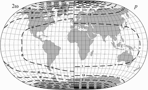
Three versions were studied for initial projections according to the chosen coefficient values of $c_2$ and $c_3$, all of them are pointed-polar pseudocylindrical with minimized distortions presented as follows. For two of them the distribution of angular and area distortions were represented on the figures, where the angular distortions were characterized, as usual, instead of $a/b$, by the maximum angular deformation $2\omega$ given by the formula$2\omega =2\cdot \arcsin \left(\frac{a-b}{a+b}\right)=2\cdot \arcsin \left(\frac{a/b-1}{a/b+1}\right),$ and the area distortions were given by p. The introduced versions with the mapping functions (1$y=\varphi ,$) and (2$c_1\cdot {\left[1-{\left(\frac{2\cdot ∥\varphi ∥}{\pi }\right)}^{c_2}\right]}^{1/c_3}\cdot \left(\lambda +c_4\cdot {\lambda }^3\right),$) are Györffy (2016, p. 262):

1. $c_2\ne 2$ and $c_3=2$ in Expression (2$c_1\cdot {\left[1-{\left(\frac{2\cdot ∥\varphi ∥}{\pi }\right)}^{c_2}\right]}^{1/c_3}\cdot \left(\lambda +c_4\cdot {\lambda }^3\right),$). The coefficients in the first row of Table 2 resulted in $E_K^2=0.13510$, $E_K=0.36756$ (Figure 1).

   The pointed-polar character of the graticule is manifested. On lower latitudes, the curvature of the map outline is zero or almost zero and the graticule can favourably fit in the rectangle of a map page.

2. $c_2=2$ and $c_3\ne 2$ in Expression (2$c_1\cdot {\left[1-{\left(\frac{2\cdot ∥\varphi ∥}{\pi }\right)}^{c_2}\right]}^{1/c_3}\cdot \left(\lambda +c_4\cdot {\lambda }^3\right),$). The second row of the Table 2 lists the coefficients resulting in $E_K^2=0.12406$, $E_K=0.35222$ (Figure 2).

   The mean overall distortion is lower, the curvature of the map outline in the environment of the poles is zero or almost zero, therefore the pointed-polar character is not so much visible, so it is more similar to a flat-polar projection.

3. $c_2\ne 2$ and $c_3\ne 2$ in Expression (2$c_1\cdot {\left[1-{\left(\frac{2\cdot ∥\varphi ∥}{\pi }\right)}^{c_2}\right]}^{1/c_3}\cdot \left(\lambda +c_4\cdot {\lambda }^3\right),$). The coefficients in the third row of the Table 2 produced $E_K^2=0.12379$, $E_K=0.35184$.

   The mean overall distortion is the lowest in this third case. The map outline is similar to the previous one, but the curvature converges to infinity approaching the Equator which causes an inconspicuous singularity on the outline.

   Figure 1. The isolines of the maximum angular deformation $2\omega \left({}^{\circ }\right)$ and the area scale p for the minimum distortion pseudocylindrical projection (a).

   

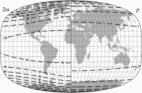
   Figure 2. The isolines of the maximum angular deformation $2\omega \left({}^{\circ }\right)$ and the area scale p for the minimum distortion pseudocylindrical projection (b).

   

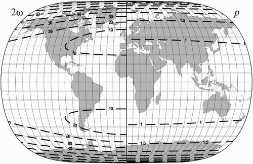
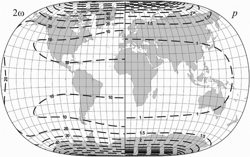
   Table 2. Coefficients $c_i$ and mean overall distortion values of the studied projections.

   proj.	$c_1$	$c_2$	$c_3$	$c_4$	$c_5$	$c_6$	$c_7$	$E_k$
   (a)	0.73044	4.20041	$2.00000$	0.00471	–	–	–	0.36756
   (b)	0.75762	$2.00000$	4.63375	0.00264	–	–	–	0.35222
   (c)	0.76158	1.67084	5.17538	0.00272	–	–	–	0.35184
   (d)	0.71416	3.79209	$2.00000$	0.00902	0.87550	0.01004	0.00273	0.34558
   (e)	0.74532	$2.00000$	4.04753	0.00730	0.93884	0.00271	0.00450	0.31959
   (f)	0.77172	$2.00000$	3.26655	0.00649	0.88525	0.00950	0.00305	0.32531

The graticule transformation presented in Section 2.3. was adapted to the foregoing minimum distortion pseudocylindrical projections (a) and (b). The criterion values arose from the two dimensional Simpson's rule (segments of $1^{\circ }$), and the coefficients $c_i$ were calculated by the downhill simplex method. The numerical results of the coefficients $c_i$, concerning (d) and (e) (corresponding to (a) and (b)), for the mapping functions (4$x=c_1\cdot {\left[1-{\left(\frac{2\cdot ∥\psi \left(\varphi ,\lambda \right)∥}{\pi }\right)}^{c_2}\right]}^{1/c_3}\cdot \left(\lambda +c_4\cdot {\lambda }^3\right),$) and (5$\begin{array}{rl}y& =\psi \left(\varphi ,\lambda \right).\end{array}$) as well as the transforming function ψ (3$\psi =\left[c_5\cdot \varphi +\left(1-c_5\right)\cdot {\left(\frac{2}{\pi }\right)}^2\cdot {\varphi }^3\right]+\left({\lambda }^2\cdot c_6+{\lambda }^4\cdot c_7\right)\cdot \left[\varphi -{\left(\frac{2}{\pi }\right)}^2\cdot {\varphi }^3\right],$) are available in the Table 2. The criterion values $E_K^2$ and $E_K$ are given below, furthermore, the distribution of the area and angular distortions are given by $2\omega$ and p on the figures:

• (d) The shape of the formula (4$x=c_1\cdot {\left[1-{\left(\frac{2\cdot ∥\psi \left(\varphi ,\lambda \right)∥}{\pi }\right)}^{c_2}\right]}^{1/c_3}\cdot \left(\lambda +c_4\cdot {\lambda }^3\right),$) is in this case:$x=c_1\cdot \sqrt{1-{\left(\frac{2\cdot ∥\psi (\varphi ,\lambda )∥}{\pi }\right)}^{c_2}}\cdot \left(\lambda +c_4\cdot {\lambda }^3\right)$and the coefficients in the fourth row of Table 2 give E_K² = 0.11943, E_K = 0.34558 (Figure 3)

• (e) The shape of the formula (4$x=c_1\cdot {\left[1-{\left(\frac{2\cdot ∥\psi \left(\varphi ,\lambda \right)∥}{\pi }\right)}^{c_2}\right]}^{1/c_3}\cdot \left(\lambda +c_4\cdot {\lambda }^3\right),$) is now:$x=c_1\cdot {\left(1-{\left(\frac{2\cdot \psi (\varphi ,\lambda )}{\pi }\right)}^2\right)}^{{\displaystyle \frac{1}{c_3}}}\cdot \left(\lambda +c_4\cdot {\lambda }^3\right)$and the coefficients in the fifth row of Table 2 results in E_K² = 0.10214, E_K = 0.31959 (Figure 4).

Figure 3. The isolines of the maximum angular deformation $2\omega \left({}^{\circ }\right)$ and the area scale p for the minimum distortion non-conical projection (d).

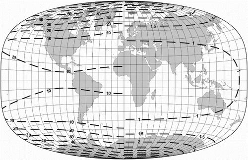
Figure 4. The isolines of the maximum angular deformation $2\omega {(}^{\circ })$ and the area scale p for the minimum distortion non-conical projection (e).

The transformation of version (c) was abandoned because there is not a notable difference between the criterion values of the version (b) and (c), and the outline of the latter has the mentioned quasi-breakpoint. So the version (a) and (b) underlies the developments.

Due to this graticule transformation, the mapped parallel curves become concave upward on the northern hemisphere and concave downward on the southern hemisphere, and their curvatures increase approaching the poles. Version (d) shows a definite pointed-polar character, while version (e) shows it less. Apart from the nominal scale, the entire length of the mapped central meridian does not change, but it is no longer divided equally by parallels, resulting in larger linear scale along the central meridian towards the poles compared to the equatorial regions. The entire length of the mapped equator is about three-quarters of the real Earth length.

Both versions of the transformed projections have a substantially reduced ($6\mathrm{\%}$ respectively $9\mathrm{\%}$) criterion value compared to the starting pseudocylindrical projections. As it is foreseeable on the basis of the pointed-polar character, the stronger distortions are concentrated at higher latitudes, while they barely increase towards the bounding meridians. Both the low angular and area distortions occur in the temperate zones, and they rise towards both the equator and the poles. The shape of the distortion isolines on the transformed maps are similar to the ones on the starting maps, but the zones of low distortions are wider.

It should be noted that the above introduced graticule transformation ψ can be applied to other types of projections, for example, to the well-known Aitoff projection, too. It shows a decline of 25% of the criterion value.

The appearance of the poles in version (e) gives a reason for reshaping the outline introduced in 2.4. The projection coefficients were calculated in the same way as previously. The results are:

• (f) According to (3$\psi =\left[c_5\cdot \varphi +\left(1-c_5\right)\cdot {\left(\frac{2}{\pi }\right)}^2\cdot {\varphi }^3\right]+\left({\lambda }^2\cdot c_6+{\lambda }^4\cdot c_7\right)\cdot \left[\varphi -{\left(\frac{2}{\pi }\right)}^2\cdot {\varphi }^3\right],$), (4$x=c_1\cdot {\left[1-{\left(\frac{2\cdot ∥\psi \left(\varphi ,\lambda \right)∥}{\pi }\right)}^{c_2}\right]}^{1/c_3}\cdot \left(\lambda +c_4\cdot {\lambda }^3\right),$) and (5$\begin{array}{rl}y& =\psi \left(\varphi ,\lambda \right).\end{array}$) where the coefficients are taken from the sixth row of the Table 2: $E_K^2=0.10583$, $E_K=0.32531$ (Figure 5).

  Figure 5. The isolines of the maximum angular deformation $2\omega {(}^{\circ })$ and the area scale p for the non-conical projection (f) derived from the projection (e) with reduced maximal outline curvature.

  

The curvature values are: ${\kappa }_{\max }=0.71586$, ${\varphi }_{{\kappa }_{\max }}={44}^{\circ }$, ${\kappa }_{\mathrm{mean}}=0.61116$, g=1.17131. (The same values before the outline correction, for the version (e) are: ${\kappa }_{\max }=0.83436$, ${\varphi }_{{\kappa }_{\max }}={57}^{\circ }$, ${\kappa }_{\mathrm{mean}}=0.62635$,$g=1.33210$.)

The distortion isolines hardly change on the whole, only the angular distortions grew somewhat at lower latitudes near the bounding meridians.

To compare the results of the upper calculations, Table 2 contains the coefficients $c_i$ of the projection equations and the mean overall distortions $E_K$ for all mentioned projections.

4. Discussion

The 16 projections reviewed in the introduction together with the 6 studied projections were compared with respect of the mean overall distortions $E_K$ and some characteristics of the outline shape.

Table 1 shows that, as expected, the reviewed conformal and equal-area projections have the highest $E_K$ value, and the aphylactic van der Grinten fits in among them. That's why these projections are not recommended for geographic world maps (Baranyi, 1987, pp. 11–12) except, at times, for cylindrical time-zone maps. The above constructed pointed-polar projections have the lowest $E_K$ value (see Table 2). If the flat-polar property is highlighted, then the Winkel Tripel is by far the best (its $E_K$ value is roughly equal to that of version (a)), and even more, the Kavrayskiy VII is also advisable, while the Robinson and the two mentioned aphylactic projections of Eckert are just on the line. If excluding the flat-polar projections, versions (d) and (f) are the main candidates with their lowest $E_K$ value, and the Baranyi IV is barely acceptable. Note that a flat-polar projection with an even slightly lower $E_K$ value can be generated by a method similar to the one presented in Section 2.2.

An accepted method measures the shape deformations on the map by the distortion of finite distances (Canters, 2002, p. 108). The distortion of distances is closely linked with the scale distortions, whose mean can be measured, for example, by the Jordan–Kavrayskiy criterion (Canters, 2002, p. 43). The correlation coefficient between the Jordan–Kavrayskiy and Airy–Kavrayskiy criteria calculated for the 23 projections reviewed equals 0.8696, which shows a close linear relationship between the two criteria. This confirms the low shape deformations of the represented objects, for example, continents, in the case of projections with minimal Airy–Kavrayskiy criterion.

The connections between the outline shapes and the mean overall distortions are worth noting. The cylindrical projections with bounding meridians as straight lines (without any curvature) have high $E_K$ value, therefore it does no good to take them into account. The projections with elliptic shape have a slightly higher $E_K$ value. The bounding meridians of Eckert III, Ortelius and van der Grinten are semicircle arcs of constant curvature, with medium or high mean overall distortions. The pointed-polar projections with minimized distortion produce the peculiar outline shape with lower curvature near the equator and the poles and higher curvature between them (see Figures 3 and 4), as introduced in Section 2.4. The shape of the mapped Earth in the renumbered Aitoff and ordinary polyconic as well as the run of the parallels in the minimized distortion pointed-polar non-conical projection together suggest that a minimized distortion projection, representing the pole as a line, generates an outline with concave pole lines similar to that mentioned above. The unfamiliar shape of the mapped Earth provokes the neglect of these projections.

In addition, the size of the angle at the intersection point of the pole line with the tangent line of the bounding meridian at its endpoint was checked. The smaller the angle is at the breakpoints, the more unfavourable they are considered. Apart from the cylindrical projections with rectangular corners, this angle is under ${150}^{\circ }$ in the case of the Eckert V. The greatest angle belongs to the Robinson $\left({165.86}^{\circ }\right)$, while the same of the Winkel and Kavrayskiy VII are between ${158}^{\circ }$ and ${163}^{\circ }$. In the case of the concavely curved pole line mentioned above, the angles are between ${100}^{\circ }$ and ${120}^{\circ }$, and it is a further aesthetic disadvantage. The bounding meridians appearing as semicircular arcs in the case of the flat-polar Eckert III and Ortelius are linked to the pole line by a smooth transition, without any breakpoint. The Mercator–Sanson is the only listed pointed-polar projection with breakpoints at the poles constructing an angle of ${144.69}^{\circ }$. The two bounding meridians of all of the others are linked at the poles smoothly. Both the advantage of the flat-polar projections and the disadvantage of the Mercator–Sanson are in this regard consistent with the mean overall distortion values.

5. Conclusions

A minimum distortion pointed-polar projection was sought for world maps, without any additional restriction concerning the map graticule. The minimization of the distortions was carried out by minimization of the Airy–Kavrayskiy criterion (giving the mean overall distortion of the map), so the angular and area distortions were reduced at the same time. Such a projection is inevitably aphylactic and non-conical. Some examples of aphylactic pointed-polar projections often used for world maps are: van der Grinten $(E_K=0.57687)$, Aitoff $(E_K=0.5218)$, Baranyi IV. pseudocylindrical $(E_K=0.4067)$, which show that the demand of keeping distortions at a level as low as possible, is often ignored.

Starting from of a minimum distortion pointed-polar pseudocylindrical projection $(E_K=0.3522)$ and changing it to a non-conical one by a polynomial graticule transformation with suitably chosen coefficients, the mean overall distortion of a world map was reduced to $E_K=0.31959$ which shows a decrease by $9.3\mathrm{\%}$. The fall is compared to some flat-polar projections: $54\mathrm{\%}$ to the Web Mercator, $19\mathrm{\%}$ to the Robinson and $13\mathrm{\%}$ to the Winkel Tripel one, see Table 1.

Zero or very small curvature of the map-outline in the environment of the poles was raised by decreasing the maximal outline curvature, so the pointed-polar character of the map became more visible (see Figure 5). The aesthetic outline correction caused a 1.8% raise $(\mathrm{to}{E}_K=0.32531)$ of the mean overall distortion on the other hand, but even so, the shapes of the continents are kept favourably.

If the theme of the map requires first and foremost minimal overall distortions (e.g. world political map), then the projection version (e) can be suggested. In the case of such maps where the pointed-polar character is expected beyond minimal overall distortions (e.g. any world maps in school atlases), version (f) is recommended. If there is relevant information on higher latitudes (e.g. map of world wind currents) the use of version (d)) is advisable.

Disclosure statement

No potential conflict of interest was reported by the author.

ORCID

János Györffy http://orcid.org/0000-0001-5303-3090

References

- Baranyi, J. (1987). Konstruktion anschaulicher Erdabbildungen. Kartographische Nachrichten, 37(1), 11–17.
- Baranyi, J., & Györffy, J. (1989). New form-true projections in Hungarian Atlases. In Hungarian cartographical studies (pp. 75–85). Budapest: Hungarian National Committee ICA.
- [Bayeva] v, E. (1987). pep oe ococa apopaecx poe, coyex cocae ap pa. eoe ApooocLea, 31(3), 109–112.
- Beineke, D. (1991). Untersuchung zur Robinson-Abbildung und Vorschlag einer analytischen Abbildungsvorschrift. Kartographische Nachrichten, 41(3), 85–94.
- Canters, F. (2002). Small-scale map projection design. London: Taylor & Francis.
- Davis, P. J., & Rabinowitz, P. (1975). Methods of numerical integration. New York, NY: Academic Press.
- Frančula, N. (1971). Die vorteilhaftesten Abbildungen in der Atlaskartographie. Bonn: Institut für Kartographie und Topographie der Rheinischen Friedrich-Wilhelms–Universität.
- Gede, M. (2011). Optimizing the distortions of sinusoidal-elliptical composit projections. In A. Ruas (Ed.), Advances in cartography and GIScience (Vol. 2, pp. 209–225). Heidelberg: Springer.
- Grafarend, E., & Niermann, A. (1984). Beste echte Zylinderabbildungen. Kartographische Nachrichten, 34(3), 103–107.
- Györffy, J. (2016). Some remarks on the question of pseudocylindrical projections with minimum distortions for world maps. In Gartner et al. (Ed.), Progress in cartography (pp. 253–265). Switzerland: ICA, Springer International.
- [Kavrayskiy] apac, B. B. (1958). pae py. Moca: C BM.
- Kerkovits, K. (2017). Vorteilhafteste flächentreue Kegelentwürfe für unregelmässig begrenzte Gebiete. Kartographische Nachrichten, 69(3), 122–128.
- Klinghammer, I. (2015). A kartográfia alapjairól: A térképvetületek kezdetei [On the basics of cartography: The development of projections]. Geodézia és kartográfia, 67(7–8), 14–19.
- Lapaine, M., & Frančula, N. (2016). Map projection aspects. International Journal of Cartography, 2(1), 38–58. doi: 10.1080/23729333.2016.1184554
- Lelgemann, D., Kleineberg, A., & Marx, Ch. (2012). Europa in der Geographie des Ptolemaios – Die Entschlüsselung des ‘Atlas Oikumene’, Zwischen Orkney, Gibraltar und der Dinariden, Zwischen Orkney, Gibraltar und der Dinariden. Darmstadt: Wissenschaftliche Buchgesellschaft.
- Livieratos, E. (2016). The Matteo Ricci 1602 Chinese World Map: The Ptolemaean echoes. International Journal of Cartography, 2(2), 186–201. doi: 10.1080/23729333.2016.1184553
- Mitchell, P. (2007). Cartographic strategies of postmodernity: The figure of the map in contemporary theory and fiction. London: Taylor & Francis.
- Mulcahy, K. A. (2000). Two new metrics for evaluating pixel-based change in data sets of global extent due to projection transformation. Cartographica: The International Journal for Geographic Information and Geovisualization, 37(2), 1–12. doi: 10.3138/C157-258R-2202-5835
- Press, W. H., Teukolsky, S. A., Vetterling, W. T., & Flannery, B. P. (1992). Numerical recipes in FORTRAN 77. Cambridge: Cambridge University Press.
- Šavrič, B., Jenny, B., White, D., & Strebe, D. R. (2015). User preferences for world map projections. Cartography and Geographic Information Science, 42(5), 398–409. doi: 10.1080/15230406.2015.1014425
- Snyder, J. P. (1985). Computer-assisted map projection research. Washington, DC: U.S. Geological Survey Bulletin no. 1629, United States Government Printing Office.
- Snyder, J. P. (1993). Flattening the Earth: Two thousand years of map projections. Chicago: The University of Chicago Press.
- Snyder, J. P., & Voxland, P. M. (1989). An album of map projections. Washington, DC: U.S. Government Printing Office.
- Steinwand, D. R., Hutchinson, J. A., & Snyder, J. P. (1995). Map projections for global and continental data sets and an analysis of pixel distortion caused by reprojection. Photogrammetric Engineering and Remote Sensing, 61(12), 1487–1497.
- Stoker, J. J. (1989). Differential geometry. Hoboken, NJ: John Wiley & Sons.
- Szigeti, Cs., & Kerkovits, K. (2018). A vetületválasztás hatása kis méretarányú térképek olvasására [Measuring map projection's effects on the interpretation of small scale maps]. Geodézia és kartográfia, 70(2), 20–31.
- Werner, R. J. (1993). A survey of preference among nine equator-centered map projections. Cartography and Geographic Information Systems, 20(1), 31–39. doi: 10.1559/152304093782616733