Comparing finite and infinitesimal map distortion measures

ABSTRACT

The traditional way to calculate the global distortion of a given area in a map projection is to create what we call a local distortion criterion that is a function of the infinitesimal semi-axes of the Tissot's indicatrix. Some contemporary scholars criticize this method, saying that the map readers face distortion of the finite type. These researchers suggest taking plenty of simple random spherical elements (line sections, triangles) and average the distortion on them. Although the aforementioned researchers all state that their approach is something fundamentally different from the traditional method, the major disadvantage is that this method is irreproducible. Therefore, it has to be investigated whether the difference is really significant between these methods and if it is, what its nature is. At first, different distortion values are evaluated on a huge number of various projections showing the whole Earth. Correlation analysis shows that there exists a strong linear dependence between the corresponding infinitesimal and finite measures. A considerable difference can be observed if the examined area is not the whole globe rather a part of it. After optimizing a projection for different distortion measures, the isolines of equal distortion follow the boundary lines significantly closer using the traditional approach.

RÉSUMÉ

une façon classique pour calculer la distorsion globale pour une surface donnée pour une projection cartographique est de créer ce que l’on appelle un critère local de distorsion qui est une fonction des demi-axes infinitésimaux de l’indicatrice de Tissot. Certains chercheurs contemporains critiquent cette méthode, en disant que les lecteurs de carte font face à la distorsion du type fini. Ces chercheurs suggèrent de prendre de nombreux éléments sphériques aléatoires simples (sections de lignes, triangles) et de calculer leur distorsion. Bien que ces chercheurs déclarent tous que leur approche est fondamentalement différente de la méthode traditionnelle, le principal inconvénient est que leur méthode n’est pas reproductible. Ainsi, il faut examiner si la différence entre ces méthodes est vraiment significative et si c'est le cas, quelle est sa nature. Pour commencer, différentes valeurs de distorsion sont évaluées sur un grand nombre de projections différentes montrant la Terre entière. L'analyse de corrélation montre qu'il existe une forte dépendance linéaire entre les mesures infinitésimales et finies. Une différence importante peut être observée si la zone examinée n'est pas le globe entier mais seulement une partie. Après avoir optimisé une projection pour différentes mesures de distorsion, on voit que les isolignes de distorsion égale suivent les limites de manière significativement plus proche en utilisant l'approche traditionnelle.

KEYWORDS:

• Map distortion measures
• optimal projection
• distortion of finite elements
• pseudoazimuthal projection

1. Introduction

Distortions of projections are traditionally measured by Tissot's indicatrix (Tissot, 1878). Airy (1861) was the first to apply distortion criteria based on the semi-axes of Tissot's indicatrix. The theory of such infinitesimal distortions was later developed by Kavrayskiy (1934), Frančula (1971) and Meshcheryakov (1968). These studies define the overall distortion of a map as the quadratic mean of distortions measured on the infinitesimal scale and calculate them practically using integral forms.

Some scholars state that map readers face distortion of the finite type. Methods considering finite shapes should also be applied. The first publication in this topic (Fisher & Miller, 1944) chose 20 spherical triangles, projected them onto the plane and replaced the curved sides of the projected triangles with straight lines. Then the lengths of the sides, the angles and the areas were compared with those of the spherical triangles. Tobler (1964) generalized the method by using a huge number of randomly chosen spherical elements in the area of interest. Later publications (Canters, 2002; Gott III, Mugnolo, & Colley, 2007; Laskowski, 1997; Peters, 1975) tried to fine-tune the method by describing different functions of the spherical and planar quantities to correctly compute the finite distortion. A common point in these research papers is that their results consistently show a big difference between the infinitesimal and finite measures. It is in compliance with the assumption: as any conformal mapping preserves the shapes of infinitesimal objects but has visible shape distortion at finite scales, these measures should differ substantially.

These different approaches generated a scientific debate. Peters (1975) argued that Frančula calculated only areal and angular distortions and neglected the effect of linear scale. In this paper, it is showed that the areal and angular distortions of the Kavrayskiy type used by Frančula (1971) contain all information about linear scales.

Canters (2002) and Peters (1975) both state that infinitesimal measures should not be used for world maps, as the distribution of the distortions is captured only by using measurements on the finite scale. Here, a theoretical explanation will show that the finite distance method differs from the infinitesimal counterpart not by considering the ‘pattern of distortion’ but by capturing the effects of flexion and skewness. Furthermore, empirical research here shows that the effects of flexion and skewness on finite distances are negligible; and even for large distances, the method of finite distances closely resembles to its infinitesimal counterpart.

On the other hand, two major disadvantages of the finite methods are shown. Due to the random sampling, calculations are irreproducible and unreliable; and finite measures hold the risk of uneven distribution when applied for a region.

2. Definitions of criteria

2.1. Distortion criteria using Tissot's indicatrix

It is easy to calculate local linear and areal scales using the infinitesimal semi-axes a and b. In case of no distortion, these areal and linear scales are equal to 1. To express local distortion, it is useful to have a measure that shows the deviation from the state without distortion. They are called local distortion criteria. These measures must always be equal to 0 wherever no distortion occurs.

For example, as the areal scale p=ab, the simplest method to create a local areal distortion criterion is to subtract one from the scale and square it in order to eliminate negative numbers:(1) ${\epsilon }_p^2=(ab-1{)}^2.$(1)

This method was first used by Airy (1861). Bayeva (1987) showed that this method does not treat areal scales 2 and 1/2 the same, although they equally distort the map. Furthermore, areal and angular distortion measures of this type are not balanced. Therefore, Bayeva suggests using the natural logarithm instead of subtracting one:(2) ${\epsilon }_p^2={\ln }^2\left(ab\right).$(2)

Such criteria are usually referred as Kavrayskiy's type (Kavrayskiy, 1934). To treat all measures coherent, logarithms of any quantities will be used in this paper, when needed.

Some researchers think that the use of such logarithms is inappropriate in the global scale, but Frančula (1980) showed that such arguments are lack of strong scientific evidence. Requiring Bayeva's aforementioned conditions of symmetry, some rational functions may also seem appropriate. Among others, Peters (1975) and Laskowski (1997) proposed using rational functions, which can be rewritten in the general form of $|x-1|/(x+1)$. These functions also fulfil the conditions described by Bayeva. However, such kinds of measures inevitably raise problems when applying for a global scale. First, the absolute value is not a differentiable function making it impossible to effectively approximate its integral using traditional numerical integration methods. Second, the use of such functions reduces the relative impact of extreme distortion, typically present closer to the boundary of projections used for world maps, as the limit of such rational functions is one as the examined (linear or areal) scale approaches infinity or zero. Using logarithms, areal or linear scales close to zero or infinity may result in an arbitrarily great value correctly reflecting the result of extreme distortion.

In small-scale cartography, the most popular method to calculate the distortion for a region S (called global distortion criterion) is to average local values throughout the region (Meshcheryakov, 1968). As the local measure is continuous, this average can be calculated as a surface integral:(3) $E_p^2=\frac{1}{S}\int {\int }_S{\epsilon }_p^2\mathrm{d}S.$(3)

Expressed in another way:(4) $E_p=\sqrt{\frac{1}{S}\int {\int }_S{\ln }^2\left(ab\right)\mathrm{d}S.}$(4)

Calculation of angular distortion is almost the same:(5) $E_a=\sqrt{\frac{1}{S}\int {\int }_S{\ln }^2\frac{a}{b}\mathrm{d}S}.$(5)

The linear scale does not only depend on the location but also on the ϑ direction. To get a local linear distortion measure, it also has to be averaged through all directions using a closed integral (Jordan, 1896). This is the Jordan–Kavrayskiy criterion:(6) $E_l=\sqrt{\frac{1}{S}\int {\int }_S\frac{1}{2\pi }\oint {\ln }^2\left(\sqrt{a^2{\cos }^2\vartheta +b^2{\sin }^2\vartheta }\right)\mathrm{d}\vartheta \mathrm{d}S}.$(6)

It is usually desired to create a single measure that summarizes the effects of these different kinds of distortions. As Bayeva (1987) points it out, Kavrayskiy's local angular and areal distortion measures have the same scale, their average is a meaningful quantity, and is the same as the Airy–Kavrayskiy criterion multiplied by $\sqrt{2}$:(7) $E_K=\sqrt{\frac{1}{S}\int {\int }_S\frac{{\ln }^2\left(ab\right)+{\ln }^2\left(\frac{a}{b}\right)}{2}\mathrm{d}S}=\sqrt{\frac{1}{S}\int {\int }_S{\ln }^{2}a+{\ln }^{2}b\mathrm{d}S}=\sqrt{\frac{E_p^2+E_a^2}{2}}.$(7)

The Jordan–Kavraysky criterion has a different origin and scale, making it impossible to sum it simply with the other two. As a consequence, one may either use the Airy–Kavrayskiy criterion stating that the linear scale is only a result of areal scale and angular distortion, or treat the linear scale as the source of the other two distortions using the Jordan–Kavrayskiy criterion. The latter approach is quite unpopular due to the complicated triple integral.

All of these criteria (except the angular distortion) have a property that after applying a similarity transform of scale c to the projection (hence changing the nominal scale), these values all change without any visible difference on the map. A scale-independent measure may be developed by changing the nominal scale. This change in the scale is selected by minimizing the corresponding measure (Canters, 2002; Gott III et al., 2007). In case of the areal distortion and the Airy–Kavrayskiy criterion, this scale correction is(8) $\ln \frac{1}{c^2}=\frac{1}{S}\int {\int }_S\ln \left(ab\right)\mathrm{d}S.$(8)

The recommended scale-correction using the Jordan–Kavrayskiy criterion is (9) $\ln \frac{1}{c}=\frac{1}{S}\int {\int }_S\frac{1}{2\pi }\oint \ln \sqrt{a^2{\cos }^2\vartheta +b^2{\sin }^2\vartheta }\mathrm{d}\vartheta \mathrm{d}S.$(9)

Aformentioned measures will be referred to as corrected global distortion, and denoted by $E_p^{\prime },E_l^{\prime }$ and $E_K^{\prime }$ if such a scale-correction has been applied. These scale-independent values have the advantage of not being sensitive to the map scale. On the other hand, it may also be a disadvantage when doing optimization. Infinitely many projections will have the same, optimal distortion value, differing only by a similarity transformation. To have only one ‘best’ projection in a projection class, as it is desired by Meshcheryakov (1968), scale-dependent measures should be used.

Distortion measures may diverge to infinity in singular points of the map (usually in the poles). Furthermore, the resulting improper surface integral on the whole globe might also not converge in this case. So the integration limits are usually chosen at latitudes $\pm {85}^{\circ }$ (Frančula, 1971; Gede, 2011; Grafarend & Niermann, 1984).

2.2. Flexion and skewness

Tissot's distortion theorem states that every projection is locally an affine transformation, and all distortions are simply the consequences of these local transformations. However, map projections as a whole are not affine transformations, since they also have projective types of distortion, which can be measured even in the infinitesimal scale. Therefore, Goldberg and Gott introduced two other criteria: flexion and skewness (Goldberg & Gott III, 2007).

Skewness shows that when moving an infinitesimal distance dt on a geodesic with azimuth ϑ, how fast the linear scale l changes:(10) $s=\frac{1}{l}\frac{\mathrm{d}l}{\mathrm{d}t}.$(10)

It is clear from this formula that s = 0 along lines with constant scale. It is impossible to create a projection without skewness: if such projection existed, it would have constant scale in all points and in all directions, so it would not have any distortion at all.

On the other hand, flexion analyses the orthogonal component of the scale variation. It is the α turn (in radians) that is taken on the map when moving along a geodesic with ϑ azimuth and dt length on the generating globe:(11) $f=\frac{\mathrm{d}\alpha }{\mathrm{d}t}.$(11)

Definition makes it clear that if a geodesic is projected to a straight line, then f = 0. Moreover, when a geodesic maps itself onto a whole circle with constant scale along it, then f = 1. It is known that in the gnomonic projection every geodesic is a straight line, so it has no flexion. It is impossible to extend such a projection to show more than half of the sphere without flexion, as the Equator is a circle in the normal aspect of all azimuthal projections, so f here must be 1.

Both f and s are hard to compute, furthermore, calculation necessitates inverse projection formulas. However, Goldberg and Gott created easy to use numerical codes.

Goldberg and Gott estimated overall flexion and skewness by Monte Carlo Integration, and eliminated negative values by taking the absolute values. To enhance similarity to the traditional criteria, overall flexion and skewness are defined here as their quadratic mean throughout the examined area:(12) $\begin{array}{rl}{E}_f& =\sqrt{\frac{1}{S}\int {\int }_S\frac{1}{2\pi }\oint f^2\mathrm{d}\vartheta \mathrm{d}S},\end{array}$(12) (13) $\begin{array}{rl}{E}_s& =\sqrt{\frac{1}{S}\int {\int }_S\frac{1}{2\pi }\oint s^2\mathrm{d}\vartheta \mathrm{d}S}.\end{array}$(13)

Flexion and skewness are in similar relationship as the areal and the angular distortion: they have similar origin, and their scaling is the same. Conformal projections even have equal amount of flexion and skewness in each point. Therefore, their cumulated effect may be calculated in a manner similar to the angular and areal distortions:(14) $E_G=\sqrt{\frac{1}{S}\int {\int }_S\frac{1}{2\pi }\oint \frac{f^2+s^2}{2}\mathrm{d}\vartheta \mathrm{d}S}=\sqrt{\frac{E_f^2+E_s^2}{2}}.$(14)

2.3. Finite distortion criteria

In order to be consistent with the measures of the Kavrayskiy type, the finite distortion measures in this paper will all use the square mean of logarithms of the ratio of spherical and planar quantities. If n random point pairs are considered in the area of interest, and their distance are denoted by d on the globe and $d^{\prime }$ on the plane, then the finite distance error is defined as in Gott III et al. (2007):(15) $E_{\mathrm{\Delta }d}=\sqrt{\frac{1}{n}\sum _{i=1}^n{\ln }^2\frac{d_i^{\prime }}{d_i}},$(15) where $d^{\prime }$ is always measured along straight lines on the map, disregarding the curvature of the mapped geodesics.

Tobler (1964) calculated the finite areal error similarly, by randomly choosing spherical triangles having all their vertices within the examined area, and the sides of their planar counterparts being replaced by straight lines. Written consistently with logarithms and squares to make comparison possible:(16) $E_{\mathrm{\Delta }p}=\sqrt{\frac{1}{n}\sum _{i=1}^n{\ln }^2\frac{A_i^{\prime }}{A_i}},$(16) where A is the spherical and $A^{\prime }$ is the planar area of these triangles.

Both $E_{\mathrm{\Delta }d}$ and $E_{\mathrm{\Delta }p}$ depend on the nominal scale of the map. Their corrected, scale-independent variants are also defined after the calculations of Gott III et al. (2007) and are denoted by a prime.(17) $\begin{array}{rl}{E}_{\mathrm{\Delta }d}^{\prime }& =\sqrt{\frac{1}{n}\sum _{i=1}^n{\left(\ln \frac{d_i^{\prime }}{d_i}-\frac{1}{n}\sum _{j=1}^n\ln \frac{d_j^{\prime }}{d_j}\right)}^2},\end{array}$(17) (18) $\begin{array}{rl}{E}_{\mathrm{\Delta }p}^{\prime }& =\sqrt{\frac{1}{n}\sum _{i=1}^n{\left(\ln \frac{A_i^{\prime }}{A_i}-\frac{1}{n}\sum _{j=1}^n\ln \frac{A_j^{\prime }}{A_j}\right)}^2}.\end{array}$(18)

Measuring the shape distortion is not so straightforward. Canters, for example, mapped random spherical circles, and he examined their deviation from a circle in the projected plane.

However, using this method the stereographic projection would be free of shape distortion due to its circle-preserving attribute. This is clearly unwanted. Therefore, a new measure, the finite shape distortion is introduced with the following desired attributes:

• It is not sensitive to changing the map scale.

• Its value may be 0 if and only if the shape of the spherical element is identical to the planar one. Otherwise it reflects the degree of the deviation.

• Its scale is comparable to other measures listed here. (It should also use the logarithms of the deviations.)

The shapes of two planar triangles are identical if and only if the lengths of corresponding sides have a constant ratio. This definition is extended here to spherical triangles. (Although a spherical and a planar triangle may never have three congruent angles, they may have identical shapes according to this definition.)

If a geometric mean of a dataset with logarithmic scale is μ, then its deviation from the mean is expressed with the geometric standard deviation (Kirkwood, 1979):(19) $\sigma ={\mathrm{e}}^{\sqrt{\sum (\ln x_i-\ln \mu {)}^2/n}}.$(19) This standard deviation is dimensionless and is not dependent on the scaling. If the shape distortion (deviation) between a spherical and a planar triangle is defined as the geometric standard deviation for the ratios of the lengths of the corresponding sides, then the definition fulfils the aforementioned conditions. So the finite shape distortion on an area is (20) $E_{\mathrm{\Delta }\delta }=\sqrt{\frac{1}{n}\sum _{i=1}^n{\ln }^2{\mathrm{e}}^{\sqrt{\left({\left(\ln \left(a_i^{\prime }/a_i\right)-\ln {\mu }_i\right)}^2+{\left(\ln \left(b_i^{\prime }/b_i\right)-\ln {\mu }_i\right)}^2+{\left(\ln \left(c_i^{\prime }/c_i\right)-\ln {\mu }_i\right)}^2\right)/3}}},$(20) where $a_i$, $b_i$ and $c_i$ are the sides of a random spherical triangle having all its vertices in the examined area, $a_i^{\prime }$, $b_i^{\prime }$ and $c_i^{\prime }$ are the sides of the corresponding mapped triangle and(21) ${\mu }_i=\left[3\right]\sqrt{\frac{a_i^{\prime }}{a_i}\cdot \frac{b_i^{\prime }}{b_i}\cdot \frac{c_i^{\prime }}{c_i}}.$(21)

The formula above may be simplified as(22) $E_{\mathrm{\Delta }\delta }=\frac{1}{\sqrt{3n}}\sqrt{\sum _{i=1}^n\left({\ln }^2\frac{a_i^{\prime }}{a_i{\mu }_i}+{\ln }^2\frac{b_i^{\prime }}{b_i{\mu }_i}+{\ln }^2\frac{c_i^{\prime }}{c_i{\mu }_i}\right)}.$(22)

3. Comparison of criteria applied for the whole globe

3.1. Methodology

Distortion criteria were evaluated for 50 different projections. These projections were chosen to represent the characteristics of each major projection family. Azimuthal, cylindrical and all types of non-conical projections are also represented as well as conformal, equal-area and aphylactic ones.

Limits of integration were chosen at $\pm {85}^{\circ }$, and because of the symmetry they were practically evaluated on a half hemisphere (Gede, 2011). Surface integrals were approximated by Simpson's rule, with the interval of $1^{\circ }$.

Whenever it was not possible to avoid Monte Carlo integration, ∼100,000 random spherical triangles were generated in equal distribution. Canters (2002) showed that the maximum size of these finite elements should be constrained. This constraint should be well chosen. As this constraint is set shorter, approaching zero, the result converges to an infinitesimal measure. To overemphasize the differences between the finite and infinitesimal distortions, a greater constraint was chosen than that of Canters. The chosen 90${}^{\circ }$ is the typical size of oceans and continents, the largest objects that map users meet in small-scale maps.

Equal distribution was achieved using the following algorithm. First, three random points were generated on the sphere in uniform distribution. Then, if one of the sides was longer than the threshold, a completely new set of points were generated. Finite distances were measured between the first two generated points of each triangle.

It is important to treat finite measures with caution, as these measures are sensitive to the discontinuities of the projection. It is common to have two points that are close to each other on the sphere that are at the opposite edges of the map. (This is generally the case near the antimeridian.) This measure would show extreme error in such situations. This is unwanted, as pseudocylindrical projections with circular contour would have smaller distortion than their more appealing elliptical counterparts. These line sections should not be simply left out, as the largest distortions are usually measured at the map edge. Therefore, any affected spherical line section will be split into two parts at the boundary cut, and its length on the plane is interpreted as the sum of the lengths of these parts (Albinus, 1981). (Both parts are still considered as if they were straight lines on the map.) A user study conducted at the time of writing this article showed that the vast majority of map users treat discontinuities in a similar manner (Szigeti & Kerkovits, 2018).

Finite areal distortion was calculated based on straight line representations of each triangle side in the plane; thus there are non-negligible deviations between the spherical and planar area caused by this straight-line approximation, especially for larger triangles. As such, even for equal-area projections, finite areal distortion is different from zero. Spherical triangles were also at the discontinuities of the projection. Whenever any of the spherical triangles contains a point that is mapped to infinity (e.g. the poles in the Mercator projection), then this measure cannot be calculated in this way, hence it is undefined. Spherical triangles were also split when calculating the finite shape distortion.

Please refer to Appendix 1 to see all the calculated distortion values. Projections were classified as equivalent if $E_p=0$ and conformal if $E_a=0$.

3.2. Relations of criteria

Relations between criteria were analysed by the calculation of the correlation matrices (Table 1). Many of the correlations are very high ($>0.9$), negative correlations are rare. The only somewhat significant negative correlation is found between areal and angular distortions, but this phenomenon is well known: equal-area maps have great angular distortion, while conformal maps considerably distort areas. It is interesting that both infinitesimal and finite area distortions have high correlation with other scale-dependent measures, but their scale-independent variants do not share this attribute, their correlations are significantly lower.

Table 1. Correlation matrices for scale-dependent and scale-independent distortions.

	$E_K$	$E_p$	$E_l$	$E_{\mathrm{\Delta }d}$	$E_{\mathrm{\Delta }p}$
$E_K$	1	0.7537	0.9694	0.9601	0.9042
$E_p$	0.7537	1	0.8834	0.9017	0.9294
$E_l$	0.9694	0.8834	1	0.997	0.9612
$E_{\mathrm{\Delta }d}$	0.9601	0.9017	0.997	1	0.9711
$E_{\mathrm{\Delta }p}$	0.9042	0.9294	0.9612	0.9711	1
	$E_a$	$E_K^{\prime }$	$E_p^{\prime }$	$E_l^{\prime }$	$E_f$	$E_s$	$E_G$	$E_{\mathrm{\Delta }\delta }$	$E_{\mathrm{\Delta }d}^{\prime }$	$E_{\mathrm{\Delta }p}^{\prime }$
$E_a$	1	0.6296	−0.5918	0.262	0.5895	0.3986	0.5749	0.5867	0.219	0.0566
$E_K^{\prime }$	0.6296	1	0.1615	0.8867	0.5673	0.5131	0.6183	0.9397	0.8672	0.6367
$E_p^{\prime }$	−0.5918	0.1615	1	0.5871	−0.1476	0.0176	−0.0872	0.2258	0.6125	0.6557
$E_l^{\prime }$	0.262	0.8867	0.5871	1	0.4068	0.4645	0.4929	0.8783	0.9938	0.8612
$E_f$	0.5895	0.5673	−0.1476	0.4068	1	0.575	0.8688	0.6633	0.3881	−0.0583
$E_s$	0.3986	0.5131	0.0176	0.4645	0.575	1	0.8997	0.5684	0.4496	0.0494
$E_G$	0.5749	0.6183	−0.0872	0.4929	0.8688	0.8997	1	0.7046	0.4716	−0.019
$E_{\mathrm{\Delta }\delta }$	0.5867	0.9397	0.2258	0.8783	0.6633	0.5684	0.7046	1	0.8662	0.5448
$E_{\mathrm{\Delta }d}^{\prime }$	0.219	0.8672	0.6125	0.9938	0.3881	0.4496	0.4716	0.8662	1	0.8609
$E_{\mathrm{\Delta }p}^{\prime }$	0.0566	0.6367	0.6557	0.8612	−0.0583	0.0494	−0.019	0.5448	0.8609	1

Goldberg's flexion and skewness are also outstanding. They have no other similar quantity, their correlations are low. Only the correlation between the distortion observed on finite shapes and the average of flexion and skewness exceeds 0.7.

In some cases, further interrelations are revealed between measures by displaying them in a coordinate system.

If the Jordan–Kavrayskiy ($E_l$) and Airy–Kavrayskiy ($E_K$) values are chosen as the horizontal and vertical axes, equal-area and conformal projections arrange into two trend lines (Figure 1a). The lower line contains the equal-area projections, conformal are in the upper line. These criteria are replaced by their corrected counterparts ($E_l^{\prime },E_K^{\prime }$) in Figure 1(b) eliminating the effect of the nominal scale. The two trend lines are still in the figure suggesting that the distortion in the local linear scale largely depends on the linear combination of the local areal and angular distortions.

Figure 1. Relations between various criteria.

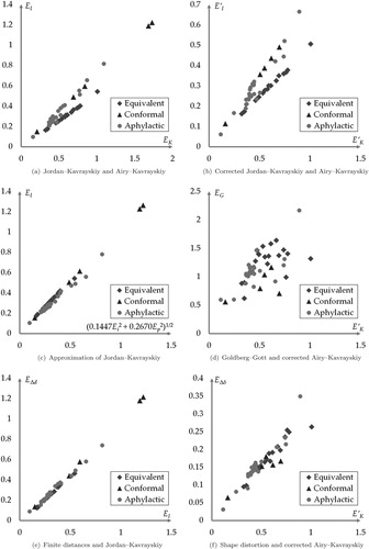
It turned out that the coefficients that fit best for the examined projections are around $E_l^2\approx 0.1447E_a^2+0.2670E_p^2$. The errors of this approximation are negligible for these projections. (The correlation is 0.9938.) See Figure 1(c). The result of a simulation with fictional Tissot indicatrices in log-normal distribution showed a similar result: $E_l^2\approx 0.1816E_a^2+0.2462E_p^2$. Therefore, it seems that the Jordan–Kavrayskiy criterion is almost twice as sensitive to areal distortions as to angular distortions.

The Jordan–Kavrayskiy criterion measures the linear scale, and the Airy–Kavrayskiy criterion shows the combined effect of areal scale and angular distortion. Consequently, the effect of the linear scale can be disregarded when using the Airy–Kavrayskiy criterion because the linear distortion can be deduced from areal and angular distortions.

Flexion, skewness and their average show only a weak correlation with any other examined criterion. (The correlation between the corrected Airy–Kavrayskiy criterion and the average of flexion and skewness is, for example, only 0.6183. In Figure 1(d), no trivial relationship is revealed between them.) It implies that the difference observed between the distortion on infinitesimal and finite objects is effectively captured by the measures of Goldberg and Gott III (2007).

The value of scale-dependent variant of the finite distance error $E_{\mathrm{\Delta }d}$ is approximately equal to the Jordan–Kavrayskiy criterion (see Appendix 2). (Their correlation is 0.9970.) See Figure 1(e). Their scale-independent variants $E_{\mathrm{\Delta }d}^{\prime }$ and $E_l^{\prime }$ also share this attribute. Difference between the method finite distances and the use of the corresponding infinitesimal measure was turned out to be negligible. In the following, this result is interpreted from a theoretical view.

The Jordan–Kavrayskiy criterion is the geometric quadratic mean of linear scales. Taking a random geodetic section, projecting it onto the plane, a curved line is obtained. The projected length is the integral (sum) of the linear scales along the line (Albinus, 1979). Division by the spherical length results in the average of the linear scale. Then, the quadratic mean for many random sections differs from the Jordan–Kavrayskiy criterion only by calculating local averages, thus eliminating local extreme distortions. Given that practically used projections are at least twice differentiable and well behaved, the variability of the linear scale originates exclusively from skewness (the derivative of the linear scale). The local averaging before taking the quadratic mean should theoretically result in a minor difference, if the examined line sections are short enough. Until this point, the curvature of mapped geodesics was not considered. As the mapped geodesics are replaced for straight line sections during calculation, the curvature (flexion) also affects measurement. Again, the longer the line section is, the greater the expected difference is. Thus the theoretically possible factors behind the finite distance method are the linear scale, flexion (curvature) and skewness (local variability of linear scale). Calculations here showed that even for large distances (up to 90${}^{\circ }$) the main factor is the linear scale; the effects of flexion and skewness are negligible. (See correlations in Table 1.)

The shape distortion can be correlated to the corrected criterion of Airy–Kavrayskiy (Figure 1f), but their correlation is slightly looser (0.9397). It corresponds to the experience that continents usually have more favourable shapes in projections in which the criterion of Airy–Kavrayskiy is lower.

4. Comparison of criteria applied for the Atlantic Ocean

4.1. The oblique transverse pseudoazimuthal projection

Until this point, all criteria were evaluated for the whole globe. However, it is usually desired to apply projections for huge regions of the world. To examine how finite criteria work applied to a region, the Atlantic Ocean was chosen for a case study, because there are an overwhelming number of papers regarding optimal projections for continental area, and only a few about oceans (Márton, 2006). It turned out that the pseudoazimuthal projection introduced in this section is flexible enough to be optimized for the ocean, and its distortion isolines can almost exactly follow the shape of the ocean.

If a projection maps the parallels to concentric full circles, but the meridians are not straight lines on the map, then this mapping is called a pseudoazimuthal projection. Projection formulas can be written using polar coordinates, as they are similar to true azimuthal projections, but now the polar angle ω is a function of both latitude and longitude. It is comfortable to use the polar distance instead of latitude:(23) $\delta :=\frac{\pi }{2}-\varphi .$(23)

Let(24) $\varrho :=\varrho \left(\delta \right)\omega :=\omega (\delta ,\lambda ),$(24) where ϱ is the polar radius and ω the polar angle:(25) $x=\varrho \sin \omega ,y=\varrho \cos \omega .$(25)

Pseudoazimuthal projections are quite rarely used in direct aspect. Being non-conical projections, they have six other aspects according to the nomenclature of Wray (1974). Ginzburg and Salmanova (1957) showed that distortion isolines in such projections follow an oval shape, making it really suitable to display nearly oval areas.

ϱ is an odd function of one variable, so an odd Maclaurin series can approximate the optimal function with any desired accuracy:(26) $\varrho =r_1\delta +r_3{\delta }^3+r_5{\delta }^5+\cdots$(26)

To conform to the traditions of cartography, the projection should be symmetric to both its horizontal and vertical axes. Thus the following ω is chosen for optimization:(27) $\begin{array}{rl}\omega & =\lambda +\xi =\lambda +(w_{11}\sin 2\lambda +w_{12}\sin 4\lambda +w_{13}\sin 6\lambda +\cdots )\delta \\ & +(w_{21}\sin 2\lambda +w_{22}\sin 4\lambda +\cdots ){\delta }^2+(w_{31}\sin 2\lambda \dots ){\delta }^3\dots \end{array}$(27)

The Atlantic Ocean can be approximated by an oval shape and is approximately symmetrical to the Equator. However, this oval shape is not extending to a true North–South direction, but it is tilted with about 25 degrees westwards. Therefore, the most suitable aspect of this projection is the oblique transverse. In the former projection formulas, everywhere ${\delta }^{\ast }$ is substituted for δ and ${\lambda }^{\ast }$ for λ (meaning metacoordinates). These metacoordinates are computed around the $({\varphi }_P=0,{\lambda }_P)$ metapole with prime metameridian ${\lambda }_M$, bringing two other parameters into optimization. See transformation formulae of aspects in Lapaine and Frančula (2016).

4.2. Minimum-distortion projections of the Atlantic Ocean according to differentcriteria

To demonstrate how different criteria work when not applied to the whole globe, rather to a region, this projection is optimized numerically for the Atlantic Ocean. The idea to characterize criteria by their optimal projection can also be found in Laskowski (1997). Here, the boundary of the ocean is the same as defined by the IHO; the optimization includes bays and neighbouring open seas.

Two corresponding criteria were chosen to optimize this projection for the Atlantic Ocean. The infinitesimal one was the Jordan–Kavrayskiy, and the finite one was the finite distance error, because these criteria showed the strongest relationship with each other. A corrected version of the Downhill Simplex Method was used for the optimization process (Kaczmarczyk, 1999). Simpson's rule was generalized for surface integrals over irregular areas to estimate the Jordan–Kavrayskiy criterion, as it is described in Kerkovits (2017). While determining the best projection according to the finite distance error, random point pairs were chosen within the area of the ocean. It was calculated several times, setting maximum allowed distance of random point pairs to different values: 30${}^{\circ }$, 60${}^{\circ }$ and 90${}^{\circ }$. The optimized coefficients are in Appendix 2.

Please note that the optimal projections according to the finite distances may slightly vary because of the irreproducibility of the Monte Carlo integration. The coefficients are similar after each calculation ($\pm 1\mathrm{\%}$), but the parameters of the projection aspect may change even $\pm 1^{\circ }$.

A digital map of the Atlantic Ocean was reprojected to display the properties of the optimal projections (Figures 2 and 3). There are green and violet isolines in these figures. The green lines show the maximal angular deviation and the red lines are there to display the local areal scale. Isolines are drawn only in the half of the map to enhance readability. The projection is symmetrical to the metapole, thus distortions are easily deduced in the other half.

Figure 2. The best pseudoazimuthal projections for the Atlantic Ocean according to different criteria.

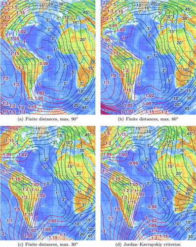
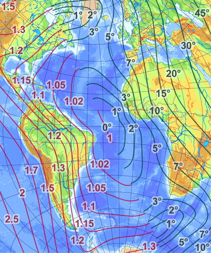
Figure 3. The best pseudoazimuthal projection for the Atlantic Ocean according to the average of flexion and skewness.

It turned out as expected that distortion isolines of the optimal projection according to the Jordan–Kavrayskiy criterion approximately follow the boundary of the area. However, the finite distance error does not have this property: as the allowed distance increases, isolines of the best projection follow the boundary less and less strictly; see Figure 2. Although, the latter projections have more favourable distortions in the centre of the map, peripheral parts (like the Gulf of Mexico) suffer bigger distortion.

As the distances were constrained shorter, the optimal projection converged to the optimal projection according to the Jordan–Kavrayskiy criterion. This strengthens the results obtained in Section 3.2: the shorter the line sections are, the stronger the influence of linear scale is.

Similar would be the result if the corrected Airy–Kavrayskiy criterion and the finite shape distortion were compared. When the maximum allowed size of spherical triangles is decreased, the distortion distribution becomes more and more even throughout the ocean, converging to the best projection according to the Airy–Kavrayskiy criterion.

This phenomenon is a consequence of how the finite methods work: the midpoint of a random line section within any area has greater probability of being in the vicinity of the geometrical centre than near the boundary. Laskowski (1997) called this the ‘edge effect’. A simple simulation can substantiate this. When a huge number of random point pairs are chosen in a rectangle, midpoints will show much lower density near the edges than in the middle, and this difference increases as the random point pairs are allowed to be further from each other.

The projection was also optimized to minimize flexion and skewness together. Because flexion and skewness are the derivatives of the local scale, and they are not sensitive to the nominal scale of the map, a boundary condition was needed: constant $r_1$ was set to 1, hence no distortion is in the metapole. Distortion isolines in the resulting projection (Figure 3) follow the boundary lines the least among the projections discussed.

5. Conclusions

In contrast to earlier studies, no considerable difference is found between some finite and infinitesimal distortions of Kavrayskiy's type. Claimed differences in earlier studies might have emerged from not examining the Jordan–Kavrayskiy criterion, and from the use of rational functions in the finite distance method instead of logarithms.

Other major results of this study:

• The finite distance error gives similar value to the Jordan–Kavrayskiy criterion. One may minimize the Jordan–Kavrayskiy criterion if the mapped finite distances should correspond to the spherical distances as much as possible.

• The finite shape distortion is closely related to the Airy–Kavrayskiy criterion. To create a map showing continents or seas with low shape distortion, the Airy–Kavrayskiy criterion may also be used.

• The Jordan–Kavrayskiy criterion can be approximated as the linear combination of angular and areal distortions in global scale, with a correlation higher than 0.99. Such a high correlation means according to the fundamentals of factor analysis that this factor (i. e. the linear scale) carries no further relevant information. The effect of linear scale may be neglected if the areal scale and angular distortion is already calculated, as it does not provide considerable additional information.

• The method of finite distances has a great disadvantage that it does not treat peripheral regions equally. The optimal projection according to the criterion of Jordan–Kavrayskiy has isolines of equal distortion following the boundary of the area more closely than these isolines do when optimizing the projection for finite distances.

• A further disadvantage of this method is the irreproducibility of the Monte Carlo Integration. Even with a huge number of shapes, the calculated parameters of optimal projections may differ $\pm 1^{\circ }$ or $\pm 1\mathrm{\%}$.

• Results imply that flexion and skewness do not have close relationship with traditional measures. Though they are likely to have some common factors and even optimization results in a similar projection, these criteria might measure substantially different kinds of distortion. Low correlation with other quantities shows that these are the measures that carry the information about non-affine distortion present in maps.

Acknowledgments

The author thanks Györffy János for his valuable ideas on the topic of the research and Gercsák Gábor for improving this article with his helpful comments on an earlier version of the manuscript.

Disclosure statement

No potential conflict of interest was reported by the author.

Notes on Contributor

Kerkovits Krisztián is a PhD student in cartography. He is interested in the theory of minimum-distortion map projections.

Appendix 1. Calculated distortions for the whole globe

Table

Projection	$E_K$	$E_p$	$E_a$	$E_l$	$E_K^{\prime }$	$E_p^{\prime }$	$E_l^{\prime }$	$E_{\mathrm{\Delta }d}$	$E_{\mathrm{\Delta }p}$	$E_{\mathrm{\Delta }\delta }$	$E_{\mathrm{\Delta }d}^{\prime }$	$E_{\mathrm{\Delta }p}^{\prime }$	$E_f$	$E_s$	$E_G$
Lambert Azim. (Transverse)	1.0073	0	1.4245	0.5419	1.0073	0	0.506	0.4614	1.1688	0.2631	0.4232	1.1661	1.2157	1.4055	1.314
Postel (Transverse)	0.8698	0.8698	0.8698	0.6548	0.7477	0.6013	0.5201	0.5785	1.2859	0.2146	0.4396	1.1913	1.294	1.3256	1.3099
Lambert cylindrical	0.691	0	0.9773	0.3636	0.691	0	0.35	0.3315	0.79	0.1976	0.3029	0.7894	0.9052	1.7152	1.3714
Behrmann	0.59	0	0.8344	0.3095	0.59	0	0.3009	0.2698	0.79	0.1668	0.252	0.7894	0.9863	1.6501	1.3594
Gall–Peters	0.5535	0	0.7827	0.286	0.5535	0	0.2779	0.2446	0.79	0.172	0.233	0.7894	1.1019	1.5565	1.3485
Plate carrée	0.4886	0.4886	0.4886	0.3508	0.4413	0.3882	0.3033	0.3376	0.883	0.1622	0.2772	0.8543	0.911	1.386	1.1728
Equrectangular	0.4172	0.4172	0.4172	0.2976	0.403	0.3882	0.2814	0.2775	0.858	0.1495	0.2567	0.8543	0.9547	1.3156	1.1494
Mercator	0.691	0.9773	0	0.4886	0.549	0.7763	0.3882	0.4389	–	0.1801	0.331	–	1.0353	1.0353	1.0353
Perspectíve cylindrical	1.0926	1.4659	0.4886	0.8159	0.893	1.1645	0.6647	0.7384	–	0.3493	0.5841	–	2.1662	2.1651	2.1657
Braun	0.5208	0.667	0.3123	0.379	0.4291	0.5204	0.3083	0.3595	0.9615	0.1547	0.279	0.8993	0.9463	1.2157	1.0893
Gall	0.4154	0.5277	0.258	0.2942	0.4107	0.5204	0.292	0.2664	0.9143	0.148	0.2634	0.8993	1.0105	1.1012	1.0568
Miller	0.5534	0.7474	0.2322	0.3993	0.4452	0.5852	0.3198	0.3736	1.0106	0.1555	0.2853	0.9322	0.9599	1.1302	1.0485
Mercator–Sanson	0.6647	0	0.9401	0.34	0.6647	0	0.3247	0.2839	0.7645	0.2074	0.2734	0.7638	1.8029	1.4543	1.6379
Sanson–Wagner	0.4321	0.3222	0.5192	0.2778	0.4117	0.2635	0.2479	0.2406	0.8027	0.1384	0.2084	0.7927	1.1339	1.0548	1.0951
Kavrayskiy VI	0.4884	0	0.6908	0.2484	0.4884	0	0.242	0.2044	0.77	0.1512	0.1994	0.7692	1.4102	1.3877	1.399
Eckert V	0.4201	0.2683	0.5301	0.2476	0.4168	0.2577	0.2476	0.2088	0.8041	0.14	0.2086	0.793	1.1436	1.0529	1.0992
Eckert VI	0.494	0	0.6986	0.2511	0.494	0.0001	0.2445	0.2072	0.7703	0.1535	0.2022	0.7695	1.3972	1.3791	1.3882
Apian II	0.4607	0.2766	0.5899	0.2882	0.4446	0.2178	0.2589	0.242	0.7663	0.1465	0.2124	0.759	1.2601	1.033	1.1522
Apian–Wagner	0.4282	0.3543	0.491	0.2853	0.4011	0.2841	0.2514	0.2492	0.8053	0.135	0.2108	0.7913	1.0983	1.0682	1.0833
Mollweide	0.5337	0	0.7547	0.2722	0.5337	0	0.2641	0.2215	0.7505	0.1645	0.2162	0.7494	1.6612	1.3959	1.5343
Mollweide–Wagner	0.476	0	0.6732	0.2424	0.476	0	0.2366	0.1971	0.759	0.1449	0.1922	0.7582	1.4829	1.4405	1.4619
Eckert III	0.4035	0.3312	0.4646	0.261	0.3973	0.3161	0.2599	0.2217	0.8176	0.1352	0.2207	0.8003	1.0055	1.1204	1.0645
Eckert IV	0.4698	0.0001	0.6644	0.2405	0.4698	0	0.2351	0.1909	0.7512	0.1374	0.1852	0.7505	1.452	1.4709	1.4615
Kavrayskiy VII	0.3693	0.2921	0.433	0.2386	0.3662	0.2841	0.2317	0.2001	0.7913	0.1239	0.1941	0.7913	1.1045	0.9873	1.0476
Baranyi IV	0.4066	0.2916	0.4957	0.2574	0.4032	0.2819	0.2487	0.2146	0.7746	0.1365	0.2079	0.7745	1.2824	1.049	1.1715
Robinson	0.3929	0.2003	0.5182	0.2333	0.3922	0.1976	0.2328	0.1939	0.7751	0.1284	0.1936	0.7698	1.2262	1.1837	1.2051
Loximuthal	0.4348	0.3301	0.5189	0.2844	0.4114	0.2631	0.252	0.2436	0.7785	0.1376	0.2085	0.7678	1.1217	1.001	1.0631
Werner	0.7793	0	1.1021	0.4006	0.7793	0	0.3768	0.3488	0.9102	0.2486	0.332	0.9096	1.5927	1.1801	1.4017
Bonne	0.7386	0	1.0445	0.3794	0.7386	0	0.3591	0.3287	0.8666	0.2351	0.3144	0.866	1.6533	1.2587	1.4693
American polyconic	0.7682	0.7469	0.7888	0.551	0.6558	0.4878	0.4206	0.4918	1.1119	0.2065	0.3643	1.0047	1.1235	0.645	0.9161
War Office	0.7738	0.6285	0.8958	0.5118	0.7398	0.5404	0.4441	0.4375	1.0333	0.2328	0.3708	0.9913	1.3636	1.0065	1.1984
Equal-area polyconic	0.7618	0	1.0773	0.3898	0.7618	0	0.3666	0.3498	0.8943	0.2543	0.3343	0.8935	1.2371	0.6512	0.9886
Lagrange	0.8416	1.1903	0	0.5951	0.5042	0.7131	0.3565	0.5771	1.4039	0.1526	0.3167	0.9787	0.791	0.791	0.791
Van der Grinten I	0.5767	0.7972	0.172	0.4083	0.4413	0.5999	0.3096	0.3657	1.0191	0.1422	0.2624	0.9098	0.9114	0.7167	0.8198
Ginzburg V	0.3738	0.2036	0.4878	0.2166	0.3725	0.1988	0.2105	0.1852	0.7876	0.1285	0.1819	0.7876	1.1546	0.8616	1.0187
Aitoff	0.5219	0.2383	0.6985	0.3097	0.5022	0.1284	0.2662	0.2658	0.7911	0.1655	0.2284	0.7778	1.2824	0.8808	1.1001
Aitoff–Wagner	0.4184	0.341	0.4835	0.2736	0.3866	0.2553	0.2342	0.24	0.8143	0.1326	0.1993	0.7962	1.0806	0.9267	1.0066
Hammer	0.5792	0	0.8191	0.2946	0.5792	0	0.284	0.2505	0.7833	0.1885	0.2442	0.7823	1.4	1.0187	1.2243
Hammer–Wagner	0.4592	0	0.6494	0.2327	0.4592	0	0.2273	0.1994	0.7764	0.1511	0.1958	0.776	1.306	1.2428	1.2748
Eckert-Greifendorff	0.6119	0	0.8653	0.3129	0.6119	0	0.3009	0.2602	0.765	0.1912	0.2516	0.7641	1.7211	1.4246	1.5798
Winkel III	0.367	0.2027	0.4779	0.2112	0.367	0.2024	0.2085	0.1841	0.774	0.1299	0.1834	0.7727	1.1852	0.8412	1.0277
Lee elliptical	1.7291	2.4453	0	1.2227	0.6167	0.8721	0.4361	1.2147	2.5811	0.1563	0.4043	1.0817	0.9847	1.3208	1.1649
Eisenlohr	1.681	2.3772	0	1.1886	0.6945	0.9822	0.4911	1.1781	2.5184	0.1672	0.4593	1.1562	0.7059	0.7059	0.7059
Goode	0.3482	0	0.4924	0.1763	0.3482	0	0.1739	0.1303	0.6108	0.0982	0.128	0.6103	1.0356	0.7268	0.8946
Boggs	0.3226	0	0.4562	0.1634	0.3226	0	0.1615	0.1245	0.6172	0.0948	0.1233	0.6169	1.0394	0.6884	0.8815
Berghaus	0.3733	0.2505	0.4646	0.2079	0.3631	0.2187	0.1886	0.1532	0.9429	0.0902	0.1317	0.8863	0.9081	0.85	0.8795
William–Olsson	0.3491	0	0.4937	0.1753	0.3491	0	0.1728	0.126	0.7993	0.0967	0.1238	0.795	0.794	0.3588	0.6161
Cahill gnomonic	0.388	0.5205	0.1735	0.2729	0.2449	0.2997	0.166	0.2536	0.9159	0.0806	0.1108	0.7379	0	0.8442	0.5969
Cahill conformal	0.2108	0.2981	0	0.149	0.1608	0.2275	0.1137	0.1353	0.8048	0.0644	0.0895	0.7514	0.5587	0.5587	0.5587
Waterman	0.1577	0.1691	0.1455	0.0962	0.1141	0.0697	0.061	0.0879	0.7258	0.0309	0.042	0.7256	0.6392	0.5438	0.5934

Appendix 2. Coefficients of the optimal projections for the Atlantic Ocean

Table

Figure	$r_1$	$r_3$	$r_5$	$w_{11}$	$w_{12}$	$w_{13}$	$w_{21}$	$w_{22}$	$w_{31}$	${\lambda }_P$	${\lambda }_M$
2(a)	0.9871	−0.0030	−0.0016	−0.0717	0.0246	−0.0037	−0.0408	−0.0082	0.0365	−31.1451${}^{\circ }$	19.7945${}^{\circ }$
2(b)	0.9905	0.0065	−0.0059	−0.1245	0.0358	−0.0076	0.0073	−0.0054	0.0179	−27.8526${}^{\circ }$	22.1870${}^{\circ }$
2(c)	0.9973	0.0036	−0.0049	−0.1994	0.0476	−0.0099	0.1211	−0.0107	−0.0274	−26.3221${}^{\circ }$	24.2428${}^{\circ }$
2(d)	0.9940	0.0015	−0.0026	−0.1891	0.0450	−0.0112	0.1023	−0.0069	−0.0198	−25.5266${}^{\circ }$	23.2368${}^{\circ }$
3	1	0.0287	−0.0024	−0.1817	0.0310	−0.0076	0.0727	0.0015	−0.0144	−28.5086${}^{\circ }$	24.3099${}^{\circ }$

References

- Airy, G. B. (1861). Explanation of a projection by balance of errors for maps applying to a very large extent of the Earth's surface; and comparison of this projection with other projections. The London, Edinburgh, and Dublin Philosophical Magazine and Journal of Science, 22(149), 409–421. doi: 10.1080/14786446108643179
- Albinus, H.-J. (1979). Lokale und globale Aspekte bei Verzerrungsfunktionen kartographischer Netzentwürfe. Kartographische Nachrichten, 29(3), 90–93.
- Albinus, H.-J. (1981). Anmerkungen und Kritik zur Entfernungsverzerrung. Kartographische Nachrichten, 31, 179–83.
- Bayeva, Ye. Yu. (1987). Kriterii otsenki dostoinstva kartograficheskikh proyektsiy ispolzuemykh dlya sostavleniya kart mira. Geodeziya i Aerofotosyomka, 3, 109–112.
- Canters, F. (2002). Small-scale map projection design. London: Taylor & Francis.
- Fisher, I., & Miller, O. M. (1944). World maps and globes. New York: Essential Books.
- Frančula, N. (1971). Die vorteilhaftesten Abbildungen in der Atlaskartographie (Doctoral dissertation). Reinischen Friedrich Wilhelms Universität, Hohen Landwirtschaftlichen Fakultät.
- Frančula, N. (1980). Über die Verzerrungen in den kartographischen Abbildungen. Kartographische Nachrichten, 30(6), 214–215.
- Gede M. (2011). Optimising the distortions of sinusoidal–elliptical composite projections. Lecture notes in geoinformation and cartography advances in cartography and GIScience (Vol. 2, pp. 209–225). Berlin: Springer.
- Ginzburg, G. A., & Salmanova, T. D. (1957). Atlas dlya vybora kartograficheskikh proyekciy (No. 110.) Trudy TsNIIGAiK, Geodezizdat, Moscow.
- Goldberg, D. M., & Gott III, J. R. (2007). Flexion and skewness in map projections of the earth. Cartographica: The International Journal for Geographic Information and Geovisualization, 42(4), 297–318. doi: 10.3138/carto.42.4.297
- Gott III, J. R., Mugnolo, C., & Colley, W. N. (2007). Map projections minimizing distance errors. Cartographica: The International Journal for Geographic Information and Geovisualization, 42(3), 219–234. doi: 10.3138/carto.42.3.219
- Grafarend, E. W., & Niermann, A. (1984). Beste echte Zylinderabbildungen. Kartographische Nachrichten, 34(3), 103–107.
- Jordan, W. (1896). Der mittlere verzerrungsfehler. Z. Vermessungswesen, 25, 249–252.
- Kaczmarczyk, G. (1999). Downhill simplex method for many dimensions. Retrieved from http://paula.univ.gda.pl/∼dokgrk/simplex.html (Last accessed: 16. 03. 2002).
- Kavrayskiy, V. V. (1934). Matematicheskaya kartografiya. Redbaza Goskartotresta, Moscow & Leningrad.
- Kerkovits K. (2017). Vorteilhafteste flächentreue Kegelentwürfe für unregelmäßig begrenzte Gebiete. Kartographische Nachrichten, 67(3), 122–128.
- Kirkwood, T. B. L. (1979). Geometric means and measures of dispersion. Biometrics, 35, 908–909.
- Lapaine, M., & Frančula, N. (2016). Map projection aspects. International Journal of Cartography, 2(1), 38–58. doi: 10.1080/23729333.2016.1184554
- Laskowski, P. (1997). Part 1: Distortion-spectrum fundamentals a new tool for analyzing and visualizing map distortions. Cartographica: The International Journal for Geographic Information and Geovisualization, 34(3), 3–18. doi: 10.3138/Y51X-1590-PV21-136G
- Márton M. (2006). Die Kartographische Darstellung der Ozeane in der geänderten Projektion IV. von Baranyi. Kartographische Nachrichten, 56(3), 145–148.
- Meshcheryakov, G. A. (1968). Teoreticheskie osnovy matematicheskoy kartografii. Moscow: Nedra.
- Peters, A. B. (1975). Wie man unsere Weltkarten der Erde ähnlicher machen kann. Kartographische Nachrichten, 25(5), 173–183.
- Szigeti Cs., & Kerkovits K. (2018). A vetületválasztás hatása kis méretarányú térképek olvasására. Geodézia és Kartográfia, 70(2), 20–30.
- Tissot, A. (1878). Mémoire sur la représentation des surfaces et les projections des cartes géographiques. Nouvelles annales de mathématiques, journal des candidats aux écoles polytechnique et normale, 17, 145–163.
- Tobler, W. R. (1964). Geographical coordinate computations. Part II. Finite map projection distortions. Defense Technical Information Center, Ann Arbor, Michigan.
- Wray, T. (1974). The Seven aspects of a general map projection. Toronto: York University.