Bayesian sparsity estimation in compressive sensing with application to MR images

Abstract

The theory of compressive sensing (CS) asserts that an unknown signal $\mathbf{x}\in {\mathbb{C}}^N$ can be accurately recovered from m measurements with $m\ll N$ provided that x is sparse. Most of the recovery algorithms need the sparsity $s={\Vert \mathbf{x}\Vert }_0$ as an input. However, generally s is unknown, and directly estimating the sparsity has been an open problem. In this study, an estimator of sparsity is proposed by using Bayesian hierarchical model. Its statistical properties such as unbiasedness and asymptotic normality are proved. In the simulation study and real data study, magnetic resonance image data is used as input signal, which becomes sparse after sparsified transformation. The results from the simulation study confirm the theoretical properties of the estimator. In practice, the estimate from a real MR image can be used for recovering future MR images under the framework of CS if they are believed to have the same sparsity level after sparsification.

Keywords:

• Compressive sensing
• sparsity
• Bayesian hierarchical model
• Matérn covariance
• MRI

1 Introduction

Compressive sensing (CS) initially emerged around the year 2006 (Donoho 2006; Candès, Romberg, and Tao 2006). The aim of CS is to recover a s-sparse signal $\mathbf{x}\in {\mathbb{C}}^N$ from m noisy observations $\mathbf{y}\in {\mathbb{C}}^m$: (1) $$\mathbf{y}=A\mathbf{x}+\mathbf{e}.$$(1)

In (1), x has s nonzero elements implying that $s={\Vert \mathbf{x}\Vert }_0,A\in {\mathbb{C}}^{m\times N}$ is a measurement matrix with $m\ll N$ satisfying restricted isometry property (?, Chapter 6) and $\mathbf{e}\in {\mathbb{C}}^m$ is additive noise such that ${\Vert \mathbf{e}\Vert }_2\le \eta$ for some $\eta \ge 0$.

To recover x in (1), it can be translated into a quadratically constrained ${\ell }_1$-minimization problem: $$\underset{\mathbf{z}\in {\mathbb{C}}^N}{\text{minimize}}\hspace{1em}{\Vert \mathbf{z}\Vert }_1\hspace{1em}\text{subject}\text{to}\hspace{1em}{\Vert A\mathbf{z}-\mathbf{y}\Vert }_2\le \eta .$$

There are several specific algorithms to solve the optimization problem, e.g., orthogonal matching pursuit (OMP), compressive sampling matching pursuit (CoSaMP), iterative hard thresholding (IHT), and hard thresholding pursuit (HTP) (?, Chapter 3). All the algorithms mentioned above need sparsity s as an input. However, s is typically unknown in practice. The difficulty to recover x consists in estimating the sparsity s.

In this study, we propose a novel estimator for sparsity by using Bayesian hierarchical model (BHM). By assuming the sparsity s to be random, our target parameter is the mathematical expectation of s, E(s). The assumption of the randomness of s is reasonable in practice, since noise commonly exists in the process of acquiring signals such that it is impossible to obtain two sparse signals that are exactly the same even under the same control (Henkelman 1985). We estimate E(s) by using an observed 2D sparse image x. The unbiasedness of the estimator is derived analytically, and it can be confirmed through a simulation study. Another interesting finding is that the estimator is asymptotically normally distributed under regular conditions, which could be used to construct confidence interval of E(s). This property is also confirmed through the simulation study. In the simulation study, 2D magnetic resonance (MR) image is considered as an input signal. MR images are not sparse in general, but they are compressible (Haldar, Hernando, and Liang 2010). For instance, they can be transformed into a sparse image, x, through wavelet thresholding techniques (Prinosil, Smekal, and Bartusek 2010). In MR imaging circumstance, the measurement matrix A is a partial Fourier matrix and y is the measurements in frequency domain called k-space. In practice, once the estimate from the model is obtained for a sparsified image, it could be directly used for recovering future MR images under the framework of CS if the MR scanner can implement the wavelet thresholding techniques to sparsify the future dense images at the scanning stage and all the relevant images are believed to have the same sparsity level $(E(s))$ after sparsification, for example, but not limited to two scans of one person’s brain within a short time interval.

This article is organized as follows. The statistical theory is introduced in Sec. 2. In Sec. 3, the methods used for the simulation study and real data analysis are specified. Results are presented in Sec. 4, followed by conclusion and discussion in Sec. 5. The article is closed with proofs of the statistical properties in Appendix.

2 Theory

Since $s={\Vert \mathbf{x}\Vert }_0$, the concrete nonzero value of each element in x is not of interest. Assume that s is random, in the sense of that each element of x is randomly assigned by either zero or nonzero value. Thus, instead of s, the mathematical expectation of s, E(s), is the parameter of interest. In this section, we introduce a BHM (Cressie and Wikle 2011) to construct a new estimator for E(s) of an observed sparse image x.

BHM is a statistical model consisting of multiple layers. It is common to have three layers in the model. The first layer is data model used to model observed data, the second layer is process model used to model the unknown parameters of interest in data model, and the last one is hyperparameter model used to model unknown hyperparameters. Let $o_i=1_{(x_i\ne 0)},\text{where}1$ is the indicator function. A Bernoulli distribution can be used to describe the assumption of randomness of s: $$\text{Layer}1\hspace{1em}{o}_i|p_i\sim \text{Ber}(p_i),\hspace{1em}0<p_i<1.$$

Let $\mathbf{o}=\{o_1,o_2,\dots ,o_N\}$ and $\mathbf{p}=\{p_1,p_2,\dots ,p_N\}$, where N is the number of elements in o as well as in x.

Then a second layer is needed to describe the distribution of p_i given by $$\text{Layer}2\hspace{1em}\text{logit}(p_i)=\mu +m_i+{ϵ}_i,$$ where μ is intercept term, m_i represents structured spatial effect, and ${ϵ}_i$ represents unstructured spatial effect. It is very common to include these two types of spatial effects, since there is typically a correlated random structure that induces correlation based on neighborhood structure as well as an uncorrelated random noise that varies from pixel to pixel (Carroll et al. 2015). Let $\mathbf{m}=\{m_1,m_2,\dots ,m_N\}$ be normal distributed with common mean $0$ and precision matrix $Q(\mathit{\theta })$, i.e., $\mathbf{m}\sim N(0,Q(\mathit{\theta }))$. The precision matrix is defined as the inverse of covariance matrix of the random field. Let $\mathit{ϵ}=\{{ϵ}_1,{ϵ}_2,\dots ,{ϵ}_N\}$ be independent and identically distributed normal with common mean $0$ and precision matrix ${\tau }_{\text{iid}}·{\mathrm{I}}_N$, i.e., $\mathit{ϵ}\sim N(0,{\tau }_{\text{iid}}·{\mathrm{I}}_N)$, where ${\tau }_{\text{iid}}$ is marginal precision and ${\mathrm{I}}_N$ is an identity matrix with dimension N × N. There are several spatial models using Markov property to construct the precision matrix Q such that the random field m is called as Gaussian Markov random field (GMRF), for instance, Besag model (Besag, York, and Mollié 1991), Leroux model (Leroux, Lei, and Breslow 2000) by using neighborhood information. The advantage of using GMRF is to produce great computational benefits (Rue and Held 2005). To use such models, conditional properties of the GMRF should be specified in advance, i.e., the order of neighborhood structure. More often a GMRF with Matérn covariance is more intuitive and easier to specify for two distinct sites i and j than to specify the conditional properties, especially in geostatistics. Matérn covariance is defined as (Matérn 1960): $$\text{cov}(m_i,m_j)=\frac{{\sigma }^2}{\Gamma (\nu )\times 2^{\nu -1}}{(\kappa {\Vert i-j\Vert }_2)}^{\nu }{K}_{\nu }(\kappa {\Vert i-j\Vert }_2),$$ where $K_{\nu }$ is the modified Bessel function of the second kind, Γ is the Gamma-function, ν is a smoothness parameter, κ is a range parameter, and ${\sigma }^2$ is marginal variance. Two important properties of a random field with Matérn covariance are that the random field is stationary and isotropic (when the distance is Euclidean) and the covariance decreases as the distance between two sites i and j increases (Matérn 1960; Stein 1999). In this study, a GMRF with Matérn covariance is used. Actually, a continuous Gaussian random field with Matérn covariance function is a solution to stochastic partial differential equation (Whittle 1954, 1963), $${({\kappa }^2-\Delta )}^{\alpha /2}z(\mathbf{s})=\mathcal{W}(\mathbf{s}),\hspace{1em}\alpha =\nu +d/2,$$ where d is the dimension of the Gaussian random field $z(\mathbf{s})$ with location index s, Δ is the Laplacian operator and $\mathcal{W}(\mathbf{s})$ is a random field with Gaussian white noises. Lindgren, Rue, and Lindström (2011) have proposed that a GMRF defined on a regular unit distance lattice with a sparse precision can be used to represent a continuous Gaussian random field with Matérn covariance for $\nu \in {\mathbb{Z}}^{+}$. The sparseness of the precision matrix Q is controlled by ν. The smaller the ν is, the sparser the Q is. For example, if ν = 1, Q can be regarded as a precision matrix defined through the third order of neighborhood structure, and the nonzero values of Q are controlled by κ. $$\begin{array}{c}\text{Layer}3\hspace{1em}\text{It}\text{provides}\text{the}\text{prior}\text{distributions}\text{of}\text{the}\text{unknown}\text{hyperparameters}\\ \text{such}\text{as}\\ \mu ,\mathit{\theta }=\{\sigma ,\kappa ,\nu \}\text{and}{\tau }_{\text{iid}}.\end{array}$$

Bayesian inference is applied to obtain the posterior distribution of p, i.e., the distribution of $\mathbf{p}|\mathbf{o}$.

By using the posterior mean of p, we construct an estimator for the mean sparsity E(s): $$\widehat{E(s)}=\sum _{i=1}^{N}E\left(p_i|\mathbf{O}\right),$$ where O is a random field from which o is sampled. Its statistical properties are presented in the following propositions, of which the proofs are left in Appendix.

Proposition 1.

$\widehat{E(s)}$ is an unbiased estimator and its variance equals to the summation over all the elements of the covariance matrix of $E(\mathbf{p}|\mathbf{O})$.

Before presenting the next proposition, we introduce one definition and some notations which help to understand the proposition as well as its proof.

Definition. A

set of random variables, of which the dimension could be any positive integer, is said to be ρ-radius dependent if any two random variables in the set are independent as long as the distance between the two random variables is greater than ρ, where $\rho \ge 0$.

Remark 1.

ρ = 0 implies that the random variables are independent.

Remark 2.

Under the model setting with Matérn covariance, $\{\text{logit}(p_i),1\le i\le N\}$ are ρ-radius dependent random variables $(\rho >0)$, where the smoothing parameter ν is related to the spatial dependence ρ. For example, if ν = 1, ρ = 2 and if ν = 2, ρ = 3.

Let ${\rho }^{*}=\lceil \rho \rceil$, the smallest integer greater than or equal to ρ. Let $\varphi$ be a positive integer greater than ${\rho }^{*}$. Let n₁, n₂ be the dimensional size of a sparse image such that $n_1\times n_2=N$. And the sparse image can be divided into a set of independent squares and borders which separate the squares. Each square has dimension $(2\varphi +1)\times (2\varphi +1)$ and consists of ${(2\varphi +1)}^2$ random variables (pixels). The width of each border is ${\rho }^{*}$ and the border regions surrounding each square consist of $2(2\varphi +1){\rho }^{*}+{({\rho }^{*})}^2$ random variables. Let $n_{\text{sq}}$ be the number of squares. Let S_k be the sum of the random variables in the kth square, $S_k^B$ be the sum of the random variables in the borders surrounding the kth square, where $k=1,2,\dots ,n_{\text{sq}}$, also ${\sigma }_k^2$ be the variance of S_k and $r_k^3=E|S_k{|}^3.$

Proposition 2.

$\widehat{E(s)}$ is asymptotically normally distributed as $n_1,n_2\to \infty$, if

1. $E(p_i|\mathbf{O})$’s are absolutely continuous random variables for $1\le i\le N$, and

2. $n_{\text{sq}}\to \infty$, and $\varphi \to \infty$ at a rate slower than $n_{\text{sq}}^{1/6}$.

Remark 3.

Condition (b) says that one can choose a relatively smaller smoothness parameter ν compared to the size of the image, implying that the spatial dependence is not strong, otherwise this assumption may not hold.

Remark 4.

The asymptotics in the proposition refers to increasing-domain asymptotics. There is another type of asymptotics, i.e., infill asymptotics (fixed-domain asymptotics). The infill asymptotics can lead the spatial dependence ρ to increase rapidly as well as $\varphi$, which might break down condition (b). This is in line with what Cressie (1993) mentioned, infill asymptotics is preferable in geostatistical data, whereas increasing-domain asymptotics is often more appropriate for lattice data.

3 Methods

In this section, we briefly introduce background about MR images to be used and specify how to sparsify the images such that it can be analyzed using the BHM described in Sec. 2. Furthermore, how to set the prior distributions for the BHM and how to evaluate the performance of the estimator are also presented in this section.

3.1 Input data

Two kinds of MR images are analyzed in the study. One kind is simulated brain images with resolution 128 × 128, and the other kind is a real brain image with resolution 256 × 256. The simulated images were produced by using simulated gradient echo based dynamic contrast enhanced MRI scans at 3T with a noise level equivalent of a 12-channel head coil based on an anatomical model from BrainWeb (Aubert-Broche, Evans, and Collins 2006). Each image consisted of background/air and 13 tissue labels annotating CSF, gray matter, white matter, fat, muscle, muscle/skin, skull, vessels, connective tissue, dura matter, bone marrow, tumor necrosis, and tumor rim (Brynolfsson et al. 2014). The real brain image was acquired with a 2D spin-echo sequence on a 3T GE Signa Positron emission tomography (PET)/MR scanner.

To be able to fit the BHM to a sparsified MR image, the following question should be answered. Is the sparsity of sparsified MR image random? Assume ${\mathbf{x}}_1,{\mathbf{x}}_2$ are two sparse images transformed from two sequential scans of MR images, ${\mathbf{x}}_{{\text{MRI}}_1}\text{and}{\mathbf{x}}_{{\text{MRI}}_2}$, of the same brain under the same conditions, any slight difference between the two images may result in the positions as well as the numbers of nonzero values in ${\mathbf{x}}_1\text{and}{\mathbf{x}}_2$ are different, i.e., $s_1\ne s_2$, which implies that s is varying and can be considered as random.

3.2 Sparsification

Since MR image is not sparse in general, one discrete wavelet transform (DWT) followed by one thresholding method could be used to transform a MR image to a sparse image in wavelet domain. There are many DWT and thresholding methods can be used (Vanithamani and Umamaheswari 2011). Since this study does not focus on evaluation of the performance among these methods, DWT of Daubechies 1 with level 3 is used and followed by the hard thresholding method to eliminate the noise. The reason of using wavelet thresholding method is that wavelet transform is good at energy compaction, the smaller coefficients represent noise and larger coefficients represent the image features. DWT decomposes the image into four sub-bands in general (i.e., A, DH, DV, and DD) shown in Fig. 1.

Fig. 1 Discrete wavelet transform with three levels.

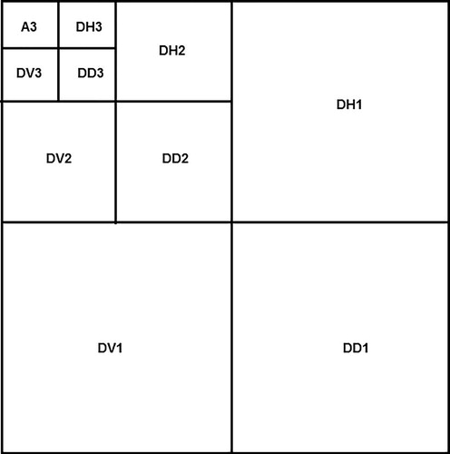
The numbers $1,2,\text{and}3$ in Fig. 1 indicate the three levels of the DWT, while DH, DV, and DD are the detail sub-bands in horizontal, vertical, and diagonal directions, respectively and A sub-band is the approximation sub-band.

The hard thresholding method eliminates coefficients that are smaller than a certain threshold value T. The function of hard thresholding is given by $$f(c)=\{\begin{array}{cc}c,\hfill & \text{if}\left|c\right|\ge T\hfill \\ 0,\hfill & \text{otherwise},\hfill \end{array}$$ where c is the detailed wavelet coefficient. Note that when the threshold value T is too small, the noise reduction is not sufficient. In the other way around, when T is too large, the noise reduction is over sufficient. In this study, one of the most commonly used method is considered to estimate the value T (Braunisch, Wu, and Kong 2000; Prinosil, Smekal, and Bartusek 2010; Vanithamani and Umamaheswari 2011), and the estimator is defined as $$\widehat{T}={\sigma }_{\text{image}}\sqrt{2\hspace{0.17em}\text{log}\hspace{0.17em}(N)},$$ where N is the number of image pixels, ${\sigma }_{\text{image}}$ is the standard deviation of noise of the image which can be estimated by Donoho (1995), Prinosil, Smekal, and Bartusek (2010), and Vanithamani and Umamaheswari (2011) $${\widehat{\sigma }}_{\text{image}}=\frac{\text{median}\left|c_D^1\right|}{0.6745},$$ where $c_D^1$ indicates detailed wavelet coefficients from level 1.

3.3 Priors of the BHM

After thresholding, a sparse image in wavelet domain is obtained. Before fitting the BHM to the sparse image, prior distributions of the unknown random variables in the third layer should be specified. A flat prior is assigned to μ which is equivalent to a Gaussian distribution with 0 precision. The priors for $\text{log}\hspace{0.17em}({\tau }_{\text{iid}})$ and $\text{log}\hspace{0.17em}(1/{\sigma }^2)$ are set to be Log-Gamma$(1,5\times {10}^{-5})$. The Log-Gamma distribution is defined as that a random variable $X\sim$ Log-Gamma(a, b) if $\text{exp}\hspace{0.17em}(X)\sim$ Gamma(a, b) (Martino and Rue 2010). Thus, a Log-Gamma(a, b) distribution is assigned to the logarithm of the precision, e.g., $\text{log}\hspace{0.17em}({\tau }_{\text{iid}})$, which is equivalent to assign a Gamma(a, b) to ${\tau }_{\text{iid}}$, and the prior knowledge about ${\tau }_{\text{iid}}$ is reflected through a and b. The prior for $\text{log}\hspace{0.17em}(\sqrt{8\nu }/\kappa )$ is set to be Log-Gamma$(1,{10}^{-2})$. $\sqrt{8\nu }/\kappa$ represents a distance where the covariance is about 0.1.

ν is treated as a fixed number. In this study, ν = 1 is used, which implies that for a pixel in the sparse image, the conditional mean of this pixel given remaining pixels is only affected by its third order nearest neighbors.

R-INLA (Rue, Martino, and Chopin 2009) is used to implement the BHM.

3.4 Evaluation

E(s) is the parameter of interest, which can also be estimated by another unbiased estimator, i.e., the sample mean $\widehat{E_{\text{sim}}(s)}=\frac{1}{n}{\sum }_{i=1}^n{s}_i$, where n is the number of simulated images and s_i is the sparsity of the ith sparse image. We use $\widehat{E_{\text{sim}}(s)}$ as a reference of the true mean value by choosing a larger value for n according to law of large numbers (LLN). A series of ${\widehat{E(s)}}_I$ can be obtained from the simulated images, which can be used to compare with $\widehat{E_{\text{sim}}(s)}$ in order to confirm the theoretical property of the unbiasedness. The unbiasedness is measured by the mean of absolute difference in percentage $|\widehat{E_{\text{sim}}(s)}-{\widehat{E(s)}}_I|*100/N$ over the series of ${\widehat{E(s)}}_I$. The range of I should not be too small in terms of LLN, whereas it should not be too large in terms of computational time. To state that the estimator is unbiased, the measurement should be close to zero. Besides the unbiasedness, the measurement also indicates the difference in terms of image size. Furthermore, the asymptotic normality of the BHM estimator could also be examined in the simulation study, since in this case $n_1=n_2=128$ (large dimensional size) and ${\rho }^{*}=2$ (weak spatial dependence), which indicates the condition (b) in Proposition 2 could be possibly met.

The evaluation methods mentioned above cannot be extended to real images analysis, since it is not practical to scan one brain even for several times. We only compare $\widehat{E(s)}$ with the true sparsity and measure the absolute difference in percentage, i.e., $|\widehat{E(s)}-s|*100/N$.

4 Results

4.1 Simulated MR images

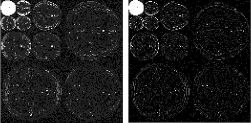
Figure 2 is one slice of simulated MR image of human brain with resolution 128 × 128. The DWT of Daubechies 1 with level 3 is shown in the left sub-figure of Fig. 3. The most upper left corner of the sub-figure is the approximation sub-band, while the remaining parts are the detail sub-bands. The estimated threshold value $\widehat{T}\approx 0.01$, implying that the detailed coefficients which are less than 0.01 are set to 0. The sparsified image is shown in the right sub-figure of Fig. 3. It is difficult to see the difference between these two sub-figures except that the right sub-figure in general is darker than the left sub-figure, which is a consequence of thresholding. From the right sub-figure in Fig. 3, it also shows that the nonzero coefficients are clustered, implying that given a pixel with higher probability to be a nonzero coefficient, its neighboring pixels should also have higher probabilities to have nonzero coefficients, and this relationship falls apart as the distance between two pixels becomes larger. This phenomenon could be described either by Matérn covariance or by its correspond sparse precision matrix. Thus, it confirms the reasonability of using BHM with Matérn covariance.

Fig. 2 A slice of simulated human brain with resolution 128 × 128.

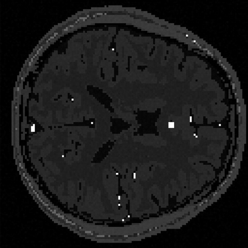
Fig. 3 Wavelet transformed image. Left: Discrete wavelet transformed image. Right: The sparsified image.

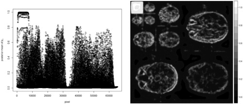
After fitting the BHM to the sparsified image, the posterior mean of p_i for each pixel can be estimated and is shown in Fig. 4.

Fig. 4 Posterior mean of p_i for every pixel Left: Scatter plot of the posterior mean of p_i. Right: Image form of the posterior mean of p_i.

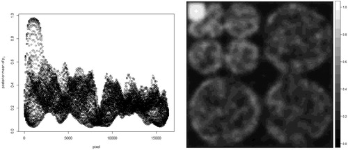
The left sub-figure of Fig. 4 is scatter plot of the posterior mean of p_i, while the right sub-figure of Fig. 4 shows the posterior mean of p_i in image form which is easier to relate the posterior mean of p_i to the sparse image in Fig. 3. It shows some pixels, located at the most upper left corner of the right sub-figure of Fig. 4, are with higher probabilities to have nonzero coefficients, while most of the remaining pixels are with lower probabilities to have nonzero coefficients. The summation of the posterior mean of p_i over all pixels, i.e., the estimator of E(s), is 4241.768. The true sparsity of the sparsified MR image is 4213. The absolute difference between the estimate and the true sparsity in percentage $|\widehat{E(s)}-s|*100/N\approx 0.2$. Afterwards, 1000 simulated MR images were generated under the same settings as the one in Fig. 2. $\widehat{E_{\text{sim}}(s)}=4219.289$ and the absolute difference between $\widehat{E_{\text{sim}}(s)}$ and the estimate in percentage $|\widehat{E_{\text{sim}}(s)}-\widehat{E(s)}|*100/N\approx 0.1$.

By far, we only illustrate the performance of the BHM estimator from a single image. Further, to evaluate the unbiasedness and stability of the estimator, 90 images out of the 1000 simulations are randomly chosen and their estimates $\widehat{E(s)}$ are calculated, respectively. The scatter plot of the absolute difference in percentage $|\widehat{E_{\text{sim}}(s)}-{\widehat{E(s)}}_I|*100/N$ for the 90 simulations, where $I=1,2,\dots ,90$, is shown in Fig. 5.

Fig. 5 $|\widehat{E_{\text{sim}}(s)}-\widehat{E(s)}|*100/N$ for 90 simulations.

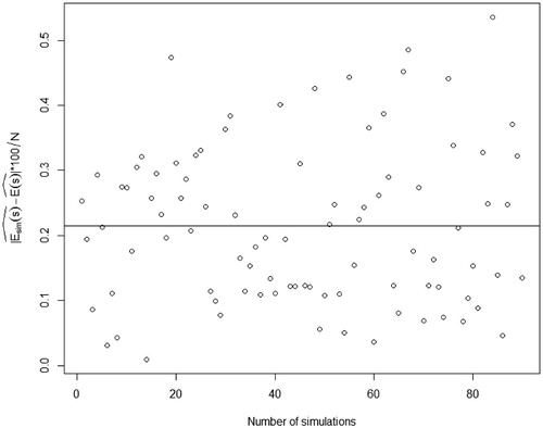
The black line is the mean of $|\widehat{E_{\text{sim}}(s)}-{\widehat{E(s)}}_I|*100/N$ over the 90 simulations, and its value is about 0.21, which is a relatively small number that could confirm the theoretical property of unbiasedness. From Fig. 5, $|\widehat{E_{\text{sim}}(s)}-\widehat{E(s)}|*100/N\in [0.01,0.53]$. The variance of $\widehat{E(s)}$ based on the 90 simulations is 480.069. All of these show that the BHM estimator from an image does not diverge too much from $\widehat{E_{\text{sim}}(s)}$. 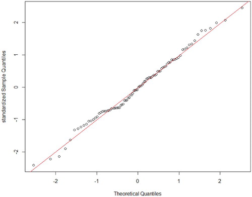Furthermore, a normal quantile-quantile plot of standardized $\widehat{E(s)}$ from the 90 simulations is shown in Fig. 6. The Shapiro–Wilk test of normality is performed and p-value $=0.7715$, implying that the estimator is normal distributed. It confirms the theoretical result about asymptotic normality of the estimator.

Fig. 6 Normal quantile-quantile plot of standardized $\widehat{E(s)}$ from 90 simulations.

4.2 Real MR image

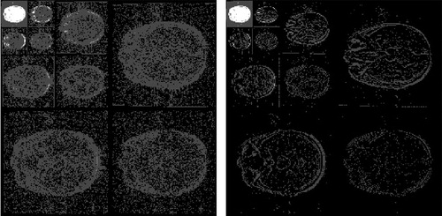
The same sparsification procedure as for the simulated images is applied here. One slice of real MR image of human brain with resolution 256 × 256 is shown in Fig. 7. The DWT of Daubechies 1 with level 3 is shown in the left sub-figure of Fig. 8. Sequentially, the hard thresholding method is used to eliminate the noise, and the result is shown in the right sub-figure of Fig. 8.

Fig. 7 One slice of real human brain with resolution 256 × 256.

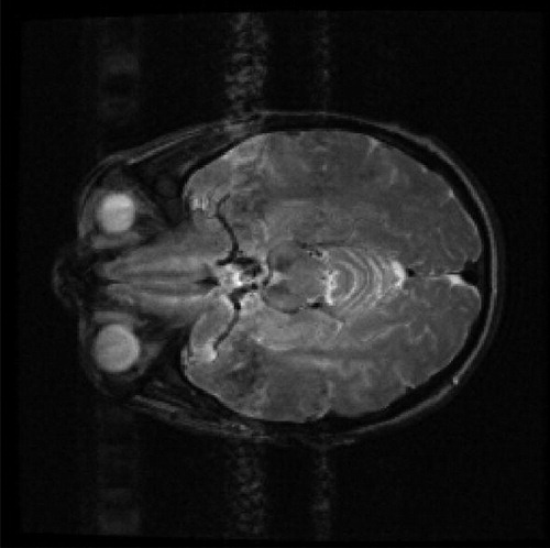
Fig. 8 Wavelet transformed image Left: Discrete wavelet transformed image. Right: The sparsified image.

By analyzing the sparsified image using the BHM, the posterior mean of p_i for each pixel is estimated and shown in Fig. 9. The left sub-figure of Fig. 9 is scatter plot of the posterior mean of p_i. The right sub-figure of Fig. 9 is the posterior mean of p_i in the image form. The summation of the posterior mean of p_i over all pixels is 8254.679. The true sparsity of the sparsified MR image is 8120. The absolute difference in percentage $|\widehat{E(s)}-s|*100/N\approx 0.2$.

Fig. 9 Posterior mean of p_i for every pixel. Left: Scatter plot of the posterior mean of p_i. Right: Image form of the posterior mean of p_i.

5 Conclusion and Discussion

In the study, we propose a novel estimator for the mathematical expectation of sparsity, E(s), and prove that it is unbiased and asymptotically normally distributed. Its variance can also be derived analytically. Simulation study is used to confirm the theoretical results. The absolute difference in percentage, i.e., $|\widehat{E_{\text{sim}}(s)}-\widehat{E(s)}|*100/N$, is about 0.21 in average, which indicates the unbiasedness. The asymptotic normality is also examined through the simulation study. The real data analysis is used for demonstration of the model and corresponding theoretical results that are not only valid for simulations, but also for real images, and illustration of the new method’s applicability in the sense of that $\widehat{E(s)}$ could be used directly in the recovery algorithms of CS for future MR images if the MR scanner can implement the wavelet thresholding techniques to sparsify the future dense images and all the relevant images are believed to have the same sparsity level after sparsification, e.g., two images of the same subject are scanned within a short time interval that could be several weeks or months. It is worth noticing that the stability of the sparsified images in terms of the sparsity is definitely related to the time interval, thus the relationship therein can be an interesting research direction.

There are some issues that are not considered in this study. Relatively conservative priors are used in the study, thus more informative priors could be used according to properties of MR images. Also different models can be used to model the GMRF, e.g., Besag and Leroux model, and comparisons are made among different models. Besides these, it is possible to fit the model to a 3D image and prove that the statistical properties still hold for 3D images. Based on the image patterns of the posterior means shown in Figs. 4 and 9, the dimension of measurement matrix, $A\in {\mathbb{C}}^{m\times N}$, is possible to be further reduced. Since if some pixels in $\mathbf{x}\in {\mathbb{C}}^N$ are believed to have zero coefficients, i.e., the probabilities are close to 0, then these pixels do not need to be measured through CS. Similarly, if some pixels are believed to possess image features, i.e., the probabilities are close to 1, then the values can be measured by a direct method rather than by CS. And CS is only applied to the remaining pixels, which leads to dimension reduction.

Acknowledgments

We would like to thank two anonymous reviewers for their detailed and insightful comments and suggestions that helped to improve the quality of the article.

Additional information

Funding

This work was supported by the Swedish Research Council grant [Reg. No.: 340-2013-5342]. The computations were performed on resources provided by the Swedish National Infrastructure for Computing (SNIC) at High Performance Computing Center North (HPC2N).

Appendix

Proof of Proposition 1.

The unbiasedness follows from the fact that $$\begin{array}{c}E\left(\widehat{E(s)}\right)=E\left(\sum _{i=1}^{N}E\left(p_i|\mathbf{O}\right)\right)=\sum _{i=1}^{N}E(p_i)=E\left(\sum _{i=1}^N{p}_i\right)=E\left(\sum _{i=1}^{N}E\left(1_{(x_i\ne 0)}|p_i\right)\right)\\ \hspace{1em}=\sum _{i=1}^{N}E\left(1_{(x_i\ne 0)}\right)=E\left(\sum _{i=1}^N{1}_{(x_i\ne 0)}\right)=E(s).\\ \text{Calculation}\text{of}\text{variance}\text{is}\text{straightforward:}\\ \text{var}\left(\widehat{E(s)}\right)=\text{var}\left(\sum _{i=1}^{N}E\left(p_i|\mathbf{O}\right)\right)=\sum _{i=1}^N\text{var}\left(E\left(p_i|\mathbf{O}\right)\right)\\ \hspace{1em}+2\sum _{1\le i<j\le N}\text{cov}\left(E\left(p_i|\mathbf{O}\right),E\left(p_j|\mathbf{O}\right)\right).\end{array}$$

□

Proof of Proposition 2.

We prove this proposition by verifying that all conditions in the theorem in Harvey, Weng, and Beckett (2010) are met, since Harvey, Weng, and Beckett (2010) have proven that the sum of ρ-radius dependent three dimensionally indexed random variables is asymptotically normally distributed under conditions. The proof for two dimensionally indexed random variables in our case follows similar to that given in Harvey, Weng, and Beckett (2010) if

1. $\{E(p_i|\mathbf{O}):1\le i\le N\}$ are ρ-radius dependent random variables, and

2. ${\sigma }_k^2$ and $r_k^3$ are finite for a given square size, and

3. $n_{\text{sq}}\to \infty$ and $\varphi \to \infty$ at a rate slower than n₁, n₂ as well as $n_{\text{sq}}$ such that (B1) $$\frac{\sum _k\text{var}(S_k^B)}{n_{\text{sq}}\sum _k{\sigma }_k^2}\to 0,$$(B1) (B2) $$\frac{{(\sum _k{r}_k^3)}^{1/3}}{{(\sum _k{\sigma }_k^2)}^{1/2}}\to 0.$$(B2)

We verify the three conditions one by one, sequentially. It has been shown that the dependence structure of a transformed GMRF is the same as the one of original GMRF if the transformed GMRF consists of absolutely continuous variables (Prates et al. 2015; Cardin 2009). Since Matérn covariance is used to model $\text{logit}(\mathbf{p})$ under the model setting, in which the random variables are ρ-radius dependent, the same dependence structure is inherited by $E(\mathbf{p}|\mathbf{O})$ if condition (a) holds, i.e., two distinct sites for $E(\mathbf{p}|\mathbf{O})$ are pairwise non-negative correlated and $\{E(p_i|\mathbf{O}):1\le i\le N\}$ are ρ-radius dependent random variables. Thus condition (i) is met.

By using the fact $0<E(p_i|\mathbf{O})<1$ almost surely, it follows that $$r_k^3=E|S_k{|}^3=E{(S_k)}^3=E{\left(\sum _{j}E\left(p_{kj}|\mathbf{O}\right)\right)}^3<{(2\varphi +1)}^6,$$ where subscript $j=1,2,\dots ,{(2\varphi +1)}^2$, subscript kj denotes the jth random variable in the kth square. Thus, $r_k^3$ is finite for a given $\varphi$, so is ${\sigma }_k^2$, and the condition (ii) is met.

Next we verify $(B1)$ and $(B2)$ which are met under condition (b). To verify $(B1)$ and $(B2)$, we need use $\text{var}(S_k^B)$ and ${\sigma }_k^2$ besides $r_k^3$ which has been shown above.

First, we calculate $\text{var}(S_k^B)$. Since $$\begin{array}{c}\text{var}\left(E\left(p_{kl}|\mathbf{O}\right)\right)<E{\left(E\left(p_{kl}|\mathbf{O}\right)\right)}^2<1,\\ \\ \text{cov}\left(E\left(p_{kl}|\mathbf{O}\right),E\left(p_{kq}|\mathbf{O}\right)\right)=E\left(E\left(p_{kl}|\mathbf{O}\right)E\left(p_{kq}|\mathbf{O}\right)\right)-E(p_{kl})E(p_{kq})\\ <E\left(E\left(p_{kl}|\mathbf{O}\right)E\left(p_{kq}|\mathbf{O}\right)\right)\\ <1,\end{array}$$ and $\varphi >{\rho }^{*}\ge 1$, it follows that $$\begin{array}{c}\text{var}(S_k^B)=\text{var}\left(\sum _{l}E\left(p_{kl}|\mathbf{O}\right)\right)=\sum _l\text{var}\left(E\left(p_{kl}|\mathbf{O}\right)\right)+\sum _{l\ne q}\text{cov}\left(E\left(p_{kl}|\mathbf{O}\right),E\left(p_{kq}|\mathbf{O}\right)\right)\\ <2(2\varphi +1){\rho }^{*}+{({\rho }^{*})}^2+[2(2\varphi +1){\rho }^{*}+{({\rho }^{*})}^2][2(2\varphi +1){\rho }^{*}+{({\rho }^{*})}^2-1]\\ =4{({\rho }^{*})}^2{(2\varphi +1)}^2+4{({\rho }^{*})}^3(2\varphi +1)+{({\rho }^{*})}^4\\ <C_1{(2\varphi +1)}^4,\end{array}$$ where $l,q=1,2,\dots ,2(2\varphi +1){\rho }^{*}+{({\rho }^{*})}^2$, C₁ is a positive constant that does not depend on n₁, n₂.

Then we calculate ${\sigma }_k^2$. Since $\{E(p_i|\mathbf{O}):1\le i\le N\}$ are ρ-radius dependent random variables and any two random variables in the set are non-negative correlated, it follows that $${\sigma }_k^2=\text{var}\left(\sum _{j}E\left(p_{kj}|\mathbf{O}\right)\right)\ge \sum _j\text{var}\left(E\left(p_{kj}|\mathbf{O}\right)\right)\ge C_2{(2\varphi +1)}^2>0,$$ where $C_2>0$ is the smallest variance of $E(p_{kj}|\mathbf{O})$ and also does not depend on n₁, n₂.

Therefore, $$\begin{array}{c}\frac{\sum _k\text{var}(S_k^B)}{n_{\text{sq}}\sum _k{\sigma }_k^2}\le \frac{n_{\text{sq}}{C}_1{(2\varphi +1)}^4}{n_{\text{sq}}^2{C}_2{(2\varphi +1)}^2}\propto \frac{{(2\varphi +1)}^2}{n_{\text{sq}}}\to 0,\text{and}\\ \frac{{(\sum _k{r}_k^3)}^{1/3}}{{(\sum _k{\sigma }_k^2)}^{1/2}}\le \frac{n_{\text{sq}}^{1/3}{(2\varphi +1)}^2}{n_{\text{sq}}^{1/2}{C}_2^{1/2}(2\varphi +1)}\propto \frac{2\varphi +1}{n_{\text{sq}}^{1/6}}\to 0,\end{array}$$ where the two limits hold if condition (b) holds. □

References

- Aubert-Broche, B., A. C. Evans, and L. Collins. 2006. “A New Improved Version of the Realistic Digital Brain Phantom.” NeuroImage 32 (1):138–45. doi: 10.1016/j.neuroimage.2006.03.052.
- Besag, J., J. York, and A. Mollié. 1991. “Bayesian Image Restoration, with Two Applications in Spatial Statistics.” Annals of the Institute of Statistical Mathematics 43 (1):1–20. doi: 10.1007/BF00116466.
- Braunisch, H., B.-I. Wu, and J. Kong. 2000. “Phase Unwrapping of SAR Interferograms after Wavelet Denoising.” IEEE Geoscience and Remote Sensing Symposium 2:752–4.
- Brynolfsson, P., J. Yu, R. Wirestam, M. Karlsson, and A. Garpebring. 2014. “Combining Phase and Magnitude Information for Contrast Agent Quantification in Dynamic Contrast-Enhanced MRI Using Statistical Modeling.” Magnetic Resonance in Medicine 74 (4):1156–64. doi: 10.1002/mrm.25490.
- Candès, E. J., J. K. Romberg, and T. Tao. 2006. “Stable Signal Recovery from Incomplete and Inaccurate Measurements.” Communications on Pure and Applied Mathematics 59 (8):1207–23. doi: 10.1002/cpa.20124.
- Cardin, M. 2009. “Multivariate Measures of Positive Dependence.” International Journal of Contemporary Mathematical Sciences 4 (4):191–200.
- Carroll, R., A. Lawson, C. Faes, R. Kirby, M. Aregay, and K. Watjou. 2015. “Comparing INLA and OpenBUGS for Hierarchical Poisson Modeling in Disease Mapping.” Spatial and Spatio-Temporal Epidemiology 14:45–54. doi: 10.1016/j.sste.2015.08.001.
- Cressie, N. 1993. Statistics for Spatial Data. New York: Wiley.
- Cressie, N., and C. K. Wikle. 2011. Statistics for Spatio-Temporal Data. Hoboken, New Jersey: Wiley.
- Donoho, D. L. 1995. “De-noising by Soft-Thresholding.” IEEE Transactions on Information Theory 41 (3):613–27. doi: 10.1109/18.382009.
- Donoho, D. L. 2006. “Compressed Sensing.” IEEE Transactions on Information Theory 52 (4):1289–306. doi: 10.1109/TIT.2006.871582.
- Foucart, S., and H. Rauhut. 2013. A Mathematical Introduction to Compressive Sensing. New York: Springer.
- Haldar, J. P., D. Hernando, and Z.-P. Liang. 2010. “Compressed-Sensing MRI with Random Encoding.” IEEE Transactions on Medical Imaging 30 (4):893–903.
- Harvey, D. J., Q. Weng, and L. A. Beckett. 2010. “On an Asymptotic Distribution of Dependent Random Variables on a 3-Dimensional Lattice.” Statistics & Probability Letters 80 (11–12):1015–21. doi: 10.1016/j.spl.2010.02.016.
- Henkelman, R. M. 1985. “Measurement of Signal Intensities in the Presence of Noise in MR Images.” Medical Physics 12 (2):232–3. doi: 10.1118/1.595711.
- Leroux, B. G., X. Lei, and N. Breslow. 2000. “Estimation of Disease Rates in Small Areas: A New Mixed Model for Spatial Dependence.” In Statistical Models in Epidemiology, the Environment, and Clinical Trials, edited by M. E. Halloran and D. Berry, 179–91. New York: Springer.
- Lindgren, F., H. Rue, and J. Lindström. 2011. “An Explicit Link between Gaussian Fields and Gaussian Markov Random Fields: The Stochastic Partial Differential Equation Approach.” Journal of the Royal Statistical Society: Series B (Statistical Methodology) 73 (4):423–98. doi: 10.1111/j.1467-9868.2011.00777.x.
- Martino, S., and H. Rue. 2010. “Implementing Approximate Bayesian Inference for Latent Gaussian Models Using Integrated Nested Laplace Approximations: A Manual for the INLA-Program.” Department of Mathematical Sciences, Norwegian University of Science and Technology.
- Matérn, B. 1960. “Spatial Variation: Stochastic Models and Their Application to Some Problems in Forest Surveys and Other Sampling Investigations.” Diss., Statens skogsforskningsinstitut, Sthlm Univ.
- Prates, M. O., D. K. Dey, M. R. Willig, and J. Yan. 2015. “Transformed Gaussian Markov Random Fields and Spatial Modeling of Species Abundance.” Spatial Statistics 14:382–99. doi: 10.1016/j.spasta.2015.07.004.
- Prinosil, J., Z. Smekal, and K. Bartusek. 2010. “Wavelet Thresholding Techniques in MRI Domain.” In Proceedings of IEEE International Conference on Biosciences, 58–63.
- Rue, H., and L. Held. 2005. Gaussian Markov Random Fields: Theory and Applications. Boca Raton: Chapman & Hall/CRC.
- Rue, H., S. Martino, and N. Chopin. 2009. “Approximate Bayesian Inference for Latent Gaussian Models by Using Integrated Nested Laplace Approximations.” Journal of the Royal Statistical Society: Series B (Statistical Methodology) 71 (2):319–92. doi: 10.1111/j.1467-9868.2008.00700.x.
- Stein, M. L. 1999. Interpolation of Spatial Data. New York: Springer-Verlag.
- Vanithamani, R., and G. Umamaheswari. 2011. “Wavelet Based Despeckling of Medical Ultrasound Images with Bilateral Filter.” In TENCON 2011—2011 IEEE Region 10 Conference.
- Whittle, P. 1954. “On Stationary Processes in the Plane.” Biometrika 41 (3–4):434. doi: 10.1093/biomet/41.3-4.434.
- Whittle, P. 1963. “Stochastic Processes in Several Dimensions.” Bulletin of the International Statistical Institute 40:974–94.