A wavelet-based approach for Johansen’s likelihood ratio test for cointegration in the presence of measurement errors: An application to CO₂ emissions and real GDP data

Abstract

We suggest a wavelet filtering technique as a remedy to the problem of measurement errors when testing for cointegration using Johansen’s (1988) likelihood ratio test. Measurement errors, which more or less are always present in empirical economic data, essentially indicates that the variable of interest (the true signal) is contaminated with noise, which may induce biased and inconsistent estimates and erroneous inference. Our Monte Carlo experiments demonstrate that measurement errors distort the statistical size of Johansen’s cointegration test in finite samples; the test is significantly oversized. A contribution and major finding of this article is that the proposed wavelet-based technique significantly improves the statistical size of the traditional Johansen test in small and medium sized samples. Since Johansen’s test is a standard cointegration test, and we demonstrate that the constantly present measurement errors in empirical data over sizes the test, this simple alteration can be used in most situations with more reliable finite sample inference. We empirically examine the long-run relation between CO₂ emissions and the real GDP in the G7 countries. The traditional Johansen tests provide evidence of an equilibrium relation for Canada and weak evidence for the US. However, the suggested size-unbiased wavelet-filtering approach consistently indicates no evidence of cointegration for all six countries.

KEYWORDS:

• Cointegration
• Johansen test
• measurement errors
• wavelets

1 Introduction

The presence of measurement errors may lead to erroneous inference in finite samples. In empirical economic data, different degrees of measurement errors are more the rule than the exception. Thus as a consequence, standard measures are often misleading. There are several plausible sources of measurement errors such as inaccuracies in data recording and inappropriate definitions used by statistical offices that do not correspond to the desired series intended for statistical or economic analysis (Haldrup, Montanes, and Sanso 2005). Moreover, variables used in usual analysis may be subject to measurement errors, for example estimated regressors in regression analysis, and estimated factors often used in dynamic factor modeling (Pagan 1984; Hong, Ahn, and Cho 2016). Other examples mentioned in the literature include situations where official statistics are compiled from survey samples and not the entire population, or where empirical variables that enter the statistical analysis are only imperfect proxies for the theoretical quantities the investigator has in mind (Nielsen 2016).

Notwithstanding the vast evidence that measurement errors can bias estimates and distort the inference, neither the econometric research community, nor the practitioners have paid much attention to it. Cragg (1994) argues that the apparent neglect of errors in variables arises for several reasons. The first reason is due to convenience; the impression that not much can be done because there are no obvious appropriate methods to deal with extra noise in the data. The second reason has its roots in the impression obtained from econometrics texts about measurement errors. Most textbooks describe the effect of measurement errors using the bivariate linear model. Employing the bivariate linear model, it has been demonstrated that measurement errors have an attenuation effect and a contamination effect. The former refers to the bias toward zero of the slope coefficients,¹ while the latter consists of the bias in the intercept of opposite sign when the average of the explanatory variable is positive.

The research development regarding non-stationary time-series has had one of the greatest impacts on econometric analysis of all time. In 1905, Karl Pearson² coined the term random walk while Yule (1926) further developed these ideas and later initialized the concept of spurious, or nonsense, regressions. At least until the 1980s, many economists applied OLS on non-stationary time series variables, which Granger and Newbold (1974) illustrated could generate spurious regressions. In 1987, the Nobel laureates Engle and Granger demonstrated that two nonstationary series can have stationary linear combinations. Following the seminal article by Engle and Granger (1987), cointegration has been a vital element of the standard toolbox for analyzing long-run macroeconomic relationships. To overcome some of the shortcomings³ of the Engle-Granger two-stage approach to cointegration, Johansen (1988, 1991) developed the maximum likelihood approach for the analysis of cointegration in VAR models with Gaussian errors.

There are some studies that have investigated the effect of measurement errors on cointegration relationships. Granger (2009) demonstrates that when two nonstationary cointegrated series are measured with errors, they are still cointegrated if all the measurement errors are I(0). However, Fischer (1990), through Monte Carlo simulation, investigates Granger’s proposition and demonstrates that measurement errors result in over rejection of the null hypothesis of no cointegration. He suggests using smaller significance level for cointegration tests when series are measured with errors, to reduce Type I error. Hassler and Kuzin (2009) through Monte Carlo simulation demonstrate that the rate of convergence of static OLS is not affected by errors in variables, but the limiting distribution does change. In a stationary framework, however, the presence of measurement errors biases the OLS estimator toward zero, the effect known as attenuation bias and does not vanish asymptotically, leading to inconsistent OLS estimates.

Hong, Ahn, and Cho (2016) investigate the effect of measurement errors on the speed-of-adjustment vector and on the cointegration vector. Their findings suggest that the reduced-rank estimator of the speed of adjustment vector is inconsistent, while that of the cointegrating vector is consistent but asymptotically biased. Nielsen (2016) extends the co-integrated vector autoregression of Johansen (1988, 1991, 1996) to the case where the variables are observed with a measurement error. Through Monte Carlo simulation, Nielsen finds that unmodeled measurement errors cause a substantial asymptotic bias in the adjustment coefficients. As a remedy, he uses a state-space form to parameterize the model, and the Kalman filter to evaluate the likelihood, and argues that after modeling measurement errors, the finite sample properties of estimators and reduced rank test statistics improve.

Duffy and Hendry (2017) analyze and simulate the impacts of integrated measurement errors on parameter estimates and tests in a bivariate cointegrated system and find that in the presence of large trends and shifts, measurement errors cause the conventional attenuation bias but do not affect much cointegration analysis.

Apart from Nielsen (2016) who attempts to provide a solution, the discussed literature contributes to the understanding of the effect of measurement errors on cointegration but does not suggest a practical way to overcome the problem. This article is an advancement in this field where we introduce a method that might be applied in finite sample. Through Monte Carlo simulation, we investigate the effect of measurement errors in variables on the size and the power of the Johansen’s trace and maximum eigenvalue tests.⁴ Unlike previous studies, we propose a wavelet-based approach to denoise series that are measured with errors to improve the size and the power of Johansen’s (1988) cointegration test. This approach is then applied to investigate the long-run relationship between CO₂ emissions and the real GDP.

However, it is important to highlight the type of errors that one is referring to. As is discussed in Morgenstern (1963) and later argued by Cragg (1994), the problem of measurement errors can refer to, but is not limited to, two main diverse types of errors. First, in the sense of mistakes in measuring an appropriately conceived quantity, and second, error in the definition of the concept being measured, so that the interpretation of the measurement does not correspond to what is actually measured. Econometricians are usually more appealed to deal with the former. The reason is that the lack of connection between the measurement and the concept being measured—which actually is a more serious problem in an economic analysis—requires the re-definition of variables. The first definition above, which is the topic of this article, refers to measurement errors in a classical⁵ sense, that is, a random error added to an otherwise appropriate measure.

The rest of the article is organized as follows. Sec. 2 discusses the econometric methods. In Sec. 3, the Monte Carlo experiment is described. Simulation results are presented and discussed in the fourth section, while Sec. 5 presents the empirical application. Sec. 6 presents the summary and conclusions.

2 Econometric methods

2.1 The likelihood ratio test and the effect of measurement errors

Consider ${\tilde{x}}_t$ a vector of observed variables that are contaminated with measurement errors:(1) $${\tilde{x}}_t=x_t+{\omega }_t$$(1) and(2) $$x_t=x_{t-1}+{\epsilon }_t$$(2) where x_t, ${\epsilon }_t$, and ω_t are K-vectors of the true signal, the error term and an additive noise, respectively; ω_t is an independent white noise process that satisfies the classical assumption.

Johansen (1988) likelihood ratio (LR) test is based on the vector error correction model (VECM) of order one (the order may be increased without any loss of generality):(3) $$\Delta {\tilde{x}}_t=\Pi {\tilde{x}}_{t-1}+{\epsilon }_t,\mathrm{t}=1,\dots ,T$$(3)

Under the null hypothesis of no cointegration, Π = 0. The Johansen’s trace statistic is obtained from the eigenvalues of the matrix (see Hassler and Kuzin 2009):(4) $${\tilde{M}}_x={\tilde{S}}_{11}^{-1}{\tilde{S}}_{10}{\tilde{S}}_{00}^{-1}{\tilde{S}}_{10}^{\prime }$$(4) where ${\tilde{S}}_{11}=T^{-1}{\sum }_{t=1}^T{\tilde{x}}_{t-1}{\tilde{x}}_{t-1}^{\prime },{\tilde{S}}_{10}=T^{-1}{\sum }_{t=1}^T{\tilde{x}}_{t-1}\Delta {\tilde{x}}_t^{\prime },{\tilde{S}}_{00}=T^{-1}{\sum }_{t=1}^T\Delta {\tilde{x}}_t\Delta {\tilde{x}}_t^{\prime }$.

The LR statistic is given by(5) $$LR=\mathit{Ttr}\left({\tilde{M}}_x\right).$$(5)

In Johansen (1988), the asymptotic distribution is derived, and it is noted that the critical values may be found and tabulated using simulation techniques. To show the effect of measurement errors on the signal to noise ratio, following Hamilton (1994), let’s rewrite Eq. (1)(1) $${\tilde{x}}_t=x_t+{\omega }_t$$(1) in first differences:$$\Delta {\tilde{x}}_t={\upsilon }_t,$$where(6) $${\upsilon }_t={\epsilon }_t+{\omega }_t+{\omega }_{t-1}.$$(6)

Then we have that:$$\begin{array}{c}E\left({\upsilon }_t\right)=0,\\ V\left({\upsilon }_t\right)={\sigma }_{\epsilon }^2+2{\sigma }_{\omega }^2,\\ Cov\left({\upsilon }_t,{\upsilon }_{t-1}\right)=-{\sigma }_{\epsilon }^2,\\ Cov\left({\upsilon }_t,{\upsilon }_{t-q}\right)=0\text{for}q>1.\end{array}$$

Then we have that ${\upsilon }_t$ follows the following MA(1) process ${\upsilon }_t={\delta }_t+\theta {\delta }_{t-1}$ where δ_t is a white noise process satisfying the classical assumptions and θ and δ_t satisfies the following:(7) $$\left(1+{\theta }^2\right){\sigma }_{\delta }^2={\sigma }_{\omega }^2+2{\sigma }_{\delta }^2\text{and}\theta =\frac{{\sigma }_{\omega }^2}{{\sigma }_{\delta }^2}.$$(7)

The signal to noise ratio may therefore be rewritten as:(8) $$\frac{{\sigma }_{\omega }}{{\sigma }_{\epsilon }}=\sqrt{\frac{\theta }{{\left(1-\theta \right)}^2}}.$$(8)

Now one may see that as $\theta \to 1$ the signal to noise ratio goes to infinity and as $\theta \to 0$ so does the signal to noise ratio too. In Hassler and Kuzin (2009), it was shown that the asymptotic distribution depends on the magnitude of this moving average parameter which is a nuisance parameter. The option suggested by Hassler and Kuzin (2009) is to estimate this nuisance parameter to solve this issue of measurement errors. However, in this article, we suggest another option which does not require any estimation of this nuisance parameter. We suggest to wavelet denoise the time series first and then use the standard Johansen (1988) test. Therefore, this approach is relatively convenient for practitioners to apply, even though we need to estimate a tuning parameter. In the next section we show how this parameter is estimated and in the simulation study it is demonstrated to work very well.

2.2 Wavelet denoising

Observed time series are often noisy. Denoising them therefore consists of removing the noise to recover the signal to be analyzed. Several methods have been suggested. The Fourier transform technique has been widely applied in different fields, such as medical imaging, signal processing, and recently in economic time series analysis. The basic premise of the FT is that any signal may be expressed as an infinite superposition of sinusoidal functions, as a linear combination of sines and cosines. However, the underlying assumption is only consistent with processes whose signals are periodic and globally stationary (Gençay, Selçuk, and Whitcher 2002).

A wavelet (small wave as opposed to sinusoids or big wave used in Fourier analysis) w(t) is local in time and local in frequency, and its oscillations damp to zero very rapidly over time. Considering that most financial and economic time series are nonstationary, the wavelet transform (WT) overcomes the limitations (poor time localization, fixed time and frequency localization) of the FT.

Consider the observed time series ${\tilde{x}}_t$ that is composed of signal and noise, as in Eq. (1)(1) $${\tilde{x}}_t=x_t+{\omega }_t$$(1) :$${\tilde{x}}_t=x_t+{\omega }_t,\hspace{1em}t=1,\dots ,T,$$where x_t is the signal and ω_t is the noise assumed to be $N(0,{\sigma }^2)$. Following Donoho and Johnstone (1994) approach x_t and ω_t can be disentangled. Extracting the signal follows several steps. The first step consists of performing the wavelet transform. The wavelet transform utilizes a basic function (mother wavelet), then dilates and translates it to capture features that are local in time and local in frequency (Gençay, Selçuk, and Whitcher 2002).

In order to calculate the scaling coefficients and the wavelet coefficients one can apply the discrete wavelet transform (DWT) or maximal overlap discrete wavelet transform (MODWT) on the time series. The MODWT has an advantage over DWT; while the DWT of level J${}_{\mathrm{o}}$ restricts the sample size to an integer multiple of 2${}_{\text{Jo}}$, there is no such limitation for the MODWT which can handle any sample size (Percival and Walden 2000; Habimana 2019). Given that the DWT requirement is rarely satisfied, we employ the MODWT.

To apply the MODWT, a discrete wavelet filter is needed. We use the Haar⁶ wavelet filter (Haar 1910). The discrete Haar filter has a length L = 2 that can be defined by its wavelet coefficients ${\tilde{w}}_j$ and scaling coefficients ${\tilde{v}}_{j,t}$. For level one, the coefficients are given by:(9) $${\tilde{w}}_{1t}=\sum _{l=1}^L{h}_l{\tilde{x}}_{t-l\mathrm{ }\text{mod}\mathrm{ }T}\text{and}{\tilde{v}}_{1t}=\sum _{l=1}^L{g}_l{\tilde{x}}_{t-l\mathrm{ }\text{mod}\mathrm{ }T,}\hspace{1em}t=1,\dots ,T$$(9) and for level two:(10) $${\tilde{w}}_{2t}=\sum _{l=1}^L{h}_l{\tilde{v}}_{1,t-l\mathrm{ }\text{mod}\mathrm{ }T}{\tilde{v}}_{2t}=\sum _{l=1}^L{g}_l{\tilde{v}}_{1,t-l\mathrm{ }\text{mod}\mathrm{ }T}\hspace{1em}t=1,\dots ,T$$(10)

The Haar wavelet is a symmetric compactly supported orthonormal wavelet, and presents the basic properties shared by most wavelet filters (Daubechies 1992; Gençay, Selçuk, and Whitcher 2002).

The scaling coefficients (${\tilde{v}}_{j,t}$, j = 1, 2) in Eqs. (9)(9) $${\tilde{w}}_{1t}=\sum _{l=1}^L{h}_l{\tilde{x}}_{t-l\mathrm{ }\text{mod}\mathrm{ }T}\text{and}{\tilde{v}}_{1t}=\sum _{l=1}^L{g}_l{\tilde{x}}_{t-l\mathrm{ }\text{mod}\mathrm{ }T,}\hspace{1em}t=1,\dots ,T$$(9) and (10)(10) $${\tilde{w}}_{2t}=\sum _{l=1}^L{h}_l{\tilde{v}}_{1,t-l\mathrm{ }\text{mod}\mathrm{ }T}{\tilde{v}}_{2t}=\sum _{l=1}^L{g}_l{\tilde{v}}_{1,t-l\mathrm{ }\text{mod}\mathrm{ }T}\hspace{1em}t=1,\dots ,T$$(10) are calculated using a weighted moving average process where g_l equals the weights. The wavelet coefficients ($\tilde{w}j$, j = 1, 2) in Eqs. (9)(9) $${\tilde{w}}_{1t}=\sum _{l=1}^L{h}_l{\tilde{x}}_{t-l\mathrm{ }\text{mod}\mathrm{ }T}\text{and}{\tilde{v}}_{1t}=\sum _{l=1}^L{g}_l{\tilde{x}}_{t-l\mathrm{ }\text{mod}\mathrm{ }T,}\hspace{1em}t=1,\dots ,T$$(9) and (10)(10) $${\tilde{w}}_{2t}=\sum _{l=1}^L{h}_l{\tilde{v}}_{1,t-l\mathrm{ }\text{mod}\mathrm{ }T}{\tilde{v}}_{2t}=\sum _{l=1}^L{g}_l{\tilde{v}}_{1,t-l\mathrm{ }\text{mod}\mathrm{ }T}\hspace{1em}t=1,\dots ,T$$(10) are calculated using a weighted difference operator where h_l equals the weights (Månsson 2012).

The wavelet coefficients are then thresholded. There are several methods for thresholding. They include universal thresholding, minimax estimation, Stein’s unbiased risk estimate, and Bayesian methods, among others. In this study we opt for universal thresholding. Donoho and Johnstone (1994) set(11) $$\delta =\sqrt{2{\widehat{\sigma }}_{\epsilon }^2\times \hspace{0.17em}\text{log}\hspace{0.17em}\left(T\right)}.$$(11)

The coefficients less than a threshold value δ are shrunk to zero. The advantage of universal thresholding is that it removes additive Gaussian noise with high probability. This corresponds to the measurement error situation since it consists of Gaussian noise.

The next step consists of selecting the thresholding rule. Nonlinear thresholding rules are preferred to linear ones because of their ability to adapt to rapidly changing nonstationary features (Donoho and Johnstone 1994; Gençay, Selçuk, and Whitcher 2002). There are two main thresholding rules: hard thresholding and soft thresholding.

Hard thresholding or ‘keep or kill’ is a straightforward and more intuitive method of denoising. The rule is stated as:(12) $$J_{jt}^{Ht}=\{\begin{array}{c}{\tilde{w}}_{jt}\mathrm{}\text{if}\mathrm{}\left|{\tilde{w}}_{jt}\right|\ge \delta \\ 0\mathrm{}\text{otherwise}\end{array},$$(12) where the threshold δ is defined in Eq. (11)(11) $$\delta =\sqrt{2{\widehat{\sigma }}_{\epsilon }^2\times \hspace{0.17em}\text{log}\hspace{0.17em}\left(T\right)}.$$(11) . Only those wavelets coefficients whose absolute values exceed the threshold are kept, and are otherwise set to zero. Hard thresholding is appropriate when there are large spikes in the observed series.

Unlike hard thresholding that pushes some coefficients toward zero and leaves others untouched, soft thresholding pushes all coefficients toward zero, and those wavelet coefficients that are smaller in magnitude than the threshold are set to zero:(13) $$J_{jt}^{st}=\mathit{sign}\left\{{\tilde{w}}_{jt}\right\}{\left(\left|{\tilde{w}}_{jt}\right|-\delta \right)}_{+},$$(13) where $J_{jt}^{st}$ are the soft wavelet denoised coefficients,(14) $$\begin{array}{c}s\mathit{ign}\left\{{\tilde{w}}_{jt}\right\}=\{\begin{array}{cc}+1& \mathrm{}\text{if}\mathrm{}{\tilde{w}}_{jt}>0\\ 0& \mathrm{}\text{if}\mathrm{}{\tilde{w}}_{jt}=0\\ -1& \mathrm{}\text{if}\mathrm{}{\tilde{w}}_{jt}<0\end{array}\hspace{1em}\text{and}\hspace{1em}\\ {\left(\left|{\tilde{w}}_{jt}\right|-\delta \right)}_{+}=\{\begin{array}{cc}\left|{\tilde{w}}_{jt}\right|-\delta & \mathrm{}\text{if}\mathrm{}\left|{\tilde{w}}_{jt}\right|-\delta \ge 0\\ 0& \mathrm{}\text{if}\mathrm{}\left|{\tilde{w}}_{jt}\right|-\delta <0\end{array}.\end{array}$$(14)

Soft thresholding is a continuous mapping. Since all wavelets are pushed toward zero, soft thresholding produces smoother estimates. However, if the observed data contain large spikes, this type of thresholding will suppress them (Gençay, Selçuk, and Whitcher 2002).

In search of a compromise between hard and soft thresholding rules, other rules have been proposed, such as Garrote’s shrinkage approach, so-called firm shrinkage, and smoothly clipped absolute deviation (SCAD) shrinkage (see Gao and Bruce 1997; Antoniadis 2007). In this article, we apply both soft and hard thresholding rules.

The final step of the algorithm consists of taking the inverse transform of the scaling coefficients and the wavelet denoised coefficients to recreate the original time series without any measurement errors. This inverse is based on the same filter as described in Eqs. (9)(9) $${\tilde{w}}_{1t}=\sum _{l=1}^L{h}_l{\tilde{x}}_{t-l\mathrm{ }\text{mod}\mathrm{ }T}\text{and}{\tilde{v}}_{1t}=\sum _{l=1}^L{g}_l{\tilde{x}}_{t-l\mathrm{ }\text{mod}\mathrm{ }T,}\hspace{1em}t=1,\dots ,T$$(9) and (10)(10) $${\tilde{w}}_{2t}=\sum _{l=1}^L{h}_l{\tilde{v}}_{1,t-l\mathrm{ }\text{mod}\mathrm{ }T}{\tilde{v}}_{2t}=\sum _{l=1}^L{g}_l{\tilde{v}}_{1,t-l\mathrm{ }\text{mod}\mathrm{ }T}\hspace{1em}t=1,\dots ,T$$(10) . Hence, g_l and h_l are used to inverse the transformation (see Gençay, Selçuk, and Whitcher 2002 for details)

3 The Monte Carlo experiments

Consider the following VECM with two series $x_{1,t}$ and $x_{2,t}$:(15) $$\begin{array}{c}\left(\begin{array}{c}\Delta x_{1,t}\\ \Delta x_{2,t}\end{array}\right)=\left(\begin{array}{c}-{\varphi }_1\hspace{1em}{\varphi }_1\\ {\varphi }_2\hspace{1em}-{\varphi }_2\end{array}\right)\left(\begin{array}{c}{x}_{1,t-1}\\ x_{2,t-1}\end{array}\right)+\left(\begin{array}{c}{\epsilon }_{1,t}\\ {\epsilon }_{2,t}\end{array}\right),\\ \hspace{1em}\text{where}\left(\begin{array}{c}{\epsilon }_{1,t}\\ {\epsilon }_{2,t}\end{array}\right)\sim \mathrm{i}.\mathrm{i}.\mathrm{d}.\mathrm{N}\left(\left[\begin{array}{c}0\\ 0\end{array}\right],\left[\begin{array}{c}1\eta \\ \eta 1\end{array}\right]\right),\end{array}$$(15) where ${\varphi }_1$ and ${\varphi }_2$ are the adjustment parameters to the equilibrium.

To incorporate measurement errors, independent and normally distributed white noise is added as follows:(16) $$\begin{array}{c}\left(\begin{array}{c}{\tilde{x}}_{1,t}\\ {\tilde{x}}_{2,t}\end{array}\right)=\left(\begin{array}{c}{x}_{1,t}\\ x_{2,t}\end{array}\right)+\left(\begin{array}{c}{\omega }_{1,t}\\ {\omega }_{2,t}\end{array}\right),\\ \hspace{1em}\text{where}\left(\begin{array}{c}{\omega }_{1,t}\\ {\omega }_{2,t}\end{array}\right)\sim \mathrm{i}.\mathrm{i}.\mathrm{d}.\mathrm{N}\left(\left[\begin{array}{c}0\\ 0\end{array}\right],\left[\begin{array}{c}\mathrm{s}0\\ 0\mathrm{s}\end{array}\right]\right).\end{array}$$(16)

Throughout the experiment, $s\in \left\{0,0.25,0.5,0.75,1\right\}$. This is a range from no measurement error up to the situation when the variance of the noise caused by the measurement error is the same as the variance of the classical error term. We limit ourselves to this range since it is not sensible in empirical situations that the variance of the measurement errors is larger than the variance of the error term. Hence, when the variance of the measurement error is equal or close to the variance of the error term, the measurement errors are considered to be large. This situation is approximately equal to Hong, Ahn, and Cho (2016) where the only difference is that they use slightly higher variance of the measurement error than the variance of error term.

To compute the size, ${\varphi }_1$ and ${\varphi }_2$ in Eq. (15)(15) $$\begin{array}{c}\left(\begin{array}{c}\Delta x_{1,t}\\ \Delta x_{2,t}\end{array}\right)=\left(\begin{array}{c}-{\varphi }_1\hspace{1em}{\varphi }_1\\ {\varphi }_2\hspace{1em}-{\varphi }_2\end{array}\right)\left(\begin{array}{c}{x}_{1,t-1}\\ x_{2,t-1}\end{array}\right)+\left(\begin{array}{c}{\epsilon }_{1,t}\\ {\epsilon }_{2,t}\end{array}\right),\\ \hspace{1em}\text{where}\left(\begin{array}{c}{\epsilon }_{1,t}\\ {\epsilon }_{2,t}\end{array}\right)\sim \mathrm{i}.\mathrm{i}.\mathrm{d}.\mathrm{N}\left(\left[\begin{array}{c}0\\ 0\end{array}\right],\left[\begin{array}{c}1\eta \\ \eta 1\end{array}\right]\right),\end{array}$$(15) are set equal to zero for the true null hypothesis of no cointegrating vector (${\varphi }_1$ = 0) for both the trace and max eigenvalue tests. And for the power ${\varphi }_1\in \left\{0.05,0.10,0.15\right\}$ to emphasize on the power of the test in the presence of near-non-cointegrated⁷ processes, and ${\phi }_2$ is set equal to zero.⁸ Since $\epsilon \sim$ N(0,1), η is equal to zero. The size and power are calculated for $T\in \left\{30,50,100,200,500\right\}$. The process is repeated 10,000 times, and the rejection frequencies are presented at a nominal level of 5%.

4 Simulation results

In this section, we present and discuss the results of the Monte Carlo experiment. The rejection frequencies of the true null hypothesis, as well as the rejection frequencies of the false null hypothesis, are reported and discussed. The former is the statistical size of the test whereas the latter represents the statistical power. The size and the power are computed for Johansen’s trace and maximum eigenvalue tests for two cases. In the first case we apply the tests on raw data, while in the second case we repeat the same tests on the same, but wavelet denoised, data.

4.1 Empirical size

Table 1 presents the rejection frequencies of the null hypothesis of no cointegration, that is, when ${\phi }_1=0$. In the Appendix we present critical values for the 5% level of significance using Eq. (15)(15) $$\begin{array}{c}\left(\begin{array}{c}\Delta x_{1,t}\\ \Delta x_{2,t}\end{array}\right)=\left(\begin{array}{c}-{\varphi }_1\hspace{1em}{\varphi }_1\\ {\varphi }_2\hspace{1em}-{\varphi }_2\end{array}\right)\left(\begin{array}{c}{x}_{1,t-1}\\ x_{2,t-1}\end{array}\right)+\left(\begin{array}{c}{\epsilon }_{1,t}\\ {\epsilon }_{2,t}\end{array}\right),\\ \hspace{1em}\text{where}\left(\begin{array}{c}{\epsilon }_{1,t}\\ {\epsilon }_{2,t}\end{array}\right)\sim \mathrm{i}.\mathrm{i}.\mathrm{d}.\mathrm{N}\left(\left[\begin{array}{c}0\\ 0\end{array}\right],\left[\begin{array}{c}1\eta \\ \eta 1\end{array}\right]\right),\end{array}$$(15) based on 10,000 replicates. We use the critical values when s = 0 (i.e. when there is no measurement errors). The empirical size is compared to the nominal size of 5% for different magnitudes of measurement errors and sample sizes. For s = 0 (series are generated without measurement errors) the Johansen performs well when applied on both raw and wavelet-denoised data. The maximum eigenvalue’s size is the closest to the nominal size, and soft thresholding performs better than hard thresholding.

Table 1 Empirical size of the Johansen cointegration test.

		Johansen (1988)		Wavelet-based Johansen test
				Soft		Hard
s	T	Trace	Max eigenvalue	Trace	Max eigenvalue	Trace	Max eigenvalue
0	30	0.047	0.047	0.049	0.050	0.049	0.046
	50	0.046	0.050	0.048	0.047	0.046	0.048
	100	0.048	0.050	0.051	0.051	0.058	0.051
	200	0.048	0.050	0.054	0.052	0.048	0.047
	500	0.051	0.052	0.049	0.050	0.054	0.052
0.25	30	0.045	0.048	0.047	0.045	0.045	0.044
	50	0.046	0.046	0.044	0.045	0.041	0.043
	100	0.047	0.045	0.047	0.047	0.051	0.047
	200	0.050	0.048	0.047	0.045	0.043	0.044
	500	0.048	0.050	0.048	0.047	0.045	0.046
0.5	30	0.047	0.045	0.037	0.037	0.040	0.041
	50	0.052	0.051	0.035	0.036	0.039	0.040
	100	0.049	0.050	0.040	0.040	0.049	0.046
	200	0.055	0.053	0.043	0.041	0.039	0.041
	500	0.055	0.059	0.042	0.042	0.043	0.045
0.75	30	0.056	0.054	0.033	0.034	0.035	0.035
	50	0.062	0.060	0.033	0.036	0.038	0.038
	100	0.075	0.071	0.041	0.040	0.043	0.040
	200	0.077	0.072	0.040	0.040	0.039	0.040
	500	0.082	0.085	0.041	0.040	0.037	0.040
1	30	0.063	0.060	0.032	0.032	0.037	0.039
	50	0.092	0.086	0.033	0.035	0.041	0.040
	100	0.115	0.110	0.044	0.045	0.049	0.047
	200	0.132	0.124	0.050	0.047	0.044	0.047
	500	0.136	0.140	0.043	0.045	0.049	0.052

The near-perfect performance of the Johansen tests in the absence of measurement errors is not surprising in this experiment since it is under the same conditions that the critical values used to compute the size were generated. When measurement errors are introduced in the data generating process (DGP), size distortion increases with s.

For s = 0.25 Johansen tests perform fairly well in both cases (raw and denoised data). The empirical sizes are still close to the nominal size. When s increases to 0.5, one can observe an uncommon situation where the size of the Johansen test is distorted, and the distortion increases with the sample size, for both the trace and the maximum eigenvalue tests. At this point, the asymptotic property of the Johansen test starts to vanish. The wavelet-based test, on the other hand, is a bit undersized in small samples (T < 100), but the size improves asymptotically; the wavelet-denoised test succeeds in rescuing the asymptotic property of the Johansen test. Both thresholding methods yield comparable results, and there are no noticeable differences between the trace and the maximum eigenvalue tests. The distortion becomes more severe when s reaches 0.75; the Johansen test is oversized, and the distortion increases with the sample size (as an example the empirical size equals 0.55 for T = 50 and it increases to 0.8 for T = 500). Measurement errors lead to the over rejection of the null hypothesis of no cointegration. However, when the data is wavelet-denoised the distortion disappears, which results in a size of 4%. Most importantly, the size distortion decreases as the sample size increases. Irrespective of the thresholding method that is used, the maximum eigenvalue test performs better, at least asymptotically.

As expected, for s = 1 the size distortion of the Johansen test is higher. Both the trace and the maximum eigenvalue tests are oversized; and this distortion increases with the sample size evaluated, from 6% for T = 50 to 14% when T = 500. However, we investigated using simulation techniques what happens if we increase the observations (we used 50,000 observations) and in the end the empirical size decreases. Hence, for very large sample sizes the standard convergence to the nominal size occurs. Denoising the data improves the size significantly, and this improvement increases with the sample size.

Overall, the presence of measurement errors distorts the size of the Johansen test. The distortion increases with the sample size for high values of s for moderate sample sizes. For the situations evaluated (which are fairly general with a wide range of observations and different magnitudes of the measurement errors), the critical values as shown in Appendix using s = 0 may be applied.

4.2 Power of the wavelet-based Johansen test

The analysis of the size of the wavelet-based Johansen test in the presence of measurement errors revealed that the test is biased, and the bias increases with the sample size; whereas the test based on the wavelet-denoised data remains unbiased.

Table 2 presents the size-adjusted power when the data are denoised using the Haar filter with soft thresholding and hard thresholding. As expected, a test with a good size comes with a cost; the test is less powerful in small samples.⁹ However, it is worth mentioning that the lower power in small samples does not come from denoising; even when series are measured without errors (s = 0), the original Johansen test is less powerful (see Table 3) for ${\phi }_1$ close to zero, that is, in the vicinity of the null hypothesis of no cointegration. The wavelet-based test exhibits very desirable properties; the power improves with the sample size, and most importantly the test is more powerful when applied to more noisy series.

Table 2 Power (size-adjusted) of the wavelet-based Johansen test.

		Soft						Hard
		Trace			Max eigenvalue			Trace			Max eigenvalue
		${\phi }_1$ = 0.05	${\phi }_1$ = 0.1	${\phi }_1$ = 0.15	${\phi }_1$ = 0.05	${\phi }_1$ = 0.10	${\phi }_1$ = 0.15	${\phi }_1$ = 0.05	${\phi }_1$ = 0.10	${\phi }_1$ = 0.15	${\phi }_1$ = 0.05	${\phi }_1$ = 0.10	${\phi }_1$ = 0.15
s	T
0	30	0.056	0.056	0.064	0.051	0.052	0.056	0.049	0.052	0.060	0.048	0.049	0.054
	50	0.055	0.070	0.085	0.053	0.063	0.074	0.051	0.067	0.081	0.050	0.060	0.074
	100	0.082	0.150	0.251	0.069	0.133	0.252	0.082	0.167	0.278	0.070	0.145	0.269
	200	0.173	0.512	0.798	0.160	0.547	0.853	0.170	0.525	0.811	0.166	0.577	0.869
	500	0.847	1.000	1.000	0.903	1.000	1.000	0.867	1.000	1.000	0.916	1.000	1.000
0.25	30	0.051	0.047	0.058	0.050	0.043	0.050	0.051	0.054	0.065	0.053	0.051	0.060
	50	0.056	0.066	0.089	0.054	0.060	0.083	0.058	0.073	0.096	0.051	0.065	0.091
	100	0.078	0.145	0.247	0.066	0.128	0.250	0.085	0.167	0.269	0.070	0.152	0.274
	200	0.198	0.568	0.834	0.176	0.582	0.872	0.180	0.552	0.845	0.166	0.588	0.888
	500	0.857	1.000	1.000	0.909	1.000	1.000	0.881	1.000	1.000	0.921	1.000	1.000
0.5	30	0.054	0.056	0.067	0.055	0.055	0.060	0.050	0.056	0.069	0.048	0.052	0.062
	50	0.056	0.070	0.094	0.053	0.060	0.082	0.058	0.083	0.104	0.053	0.070	0.094
	100	0.080	0.161	0.289	0.065	0.142	0.287	0.070	0.160	0.287	0.064	0.151	0.297
	200	0.186	0.568	0.866	0.167	0.606	0.908	0.201	0.618	0.897	0.183	0.654	0.931
	500	0.884	1.000	1.000	0.931	1.000	1.000	0.901	1.000	1.000	0.935	1.000	1.000
0.75	30	0.045	0.051	0.059	0.048	0.049	0.055	0.049	0.056	0.066	0.048	0.053	0.059
	50	0.065	0.082	0.109	0.054	0.071	0.090	0.057	0.078	0.105	0.054	0.069	0.093
	100	0.085	0.175	0.319	0.073	0.165	0.321	0.088	0.177	0.328	0.077	0.172	0.339
	200	0.183	0.600	0.898	0.178	0.662	0.939	0.196	0.639	0.917	0.190	0.691	0.955
	500	0.895	1.000	1.000	0.937	1.000	1.000	0.909	1.000	1.000	0.949	1.000	1.000
1	30	0.053	0.059	0.065	0.055	0.054	0.060	0.053	0.061	0.067	0.050	0.054	0.059
	50	0.058	0.080	0.103	0.052	0.066	0.091	0.061	0.084	0.122	0.053	0.071	0.104
	100	0.084	0.169	0.326	0.078	0.167	0.350	0.080	0.180	0.323	0.068	0.166	0.335
	200	0.201	0.631	0.918	0.178	0.667	0.947	0.220	0.665	0.938	0.212	0.712	0.963
	500	0.898	1.000	1.000	0.938	1.000	1.000	0.914	1.000	1.000	0.951	1.000	1.000

Table 3 Power (size-adjusted) of the Johansen (1988)’s test.

		Trace			Max eigenvalue
		${\phi }_1$ = 0. 05	${\phi }_1$ = 0.10	${\phi }_1$ = 0.15	${\phi }_1$ = 0.05	${\phi }_1$ = 0.10	${\phi }_1$ = 0.15
s	T
0	30	0.052	0.066	0.084	0.047	0.060	0.069
	50	0.067	0.109	0.178	0.061	0.095	0.156
	100	0.115	0.308	0.545	0.097	0.298	0.567
	200	0.345	0.836	0.986	0.332	0.870	0.993
	500	0.968	1.000	1.000	0.983	1.000	1.000
0.25	30	0.058	0.072	0.091	0.053	0.060	0.077
	50	0.077	0.119	0.183	0.063	0.101	0.164
	100	0.130	0.310	0.562	0.108	0.299	0.586
	200	0.361	0.854	0.990	0.344	0.885	0.996
	500	0.967	1.000	1.000	0.983	1.000	1.000
0.5	30	0.058	0.071	0.089	0.054	0.061	0.077
	50	0.073	0.114	0.188	0.063	0.093	0.162
	100	0.128	0.318	0.581	0.111	0.299	0.596
	200	0.348	0.843	0.992	0.325	0.875	0.997
	500	0.970	1.000	1.000	0.986	1.000	1.000
0.75	30	0.051	0.062	0.082	0.047	0.057	0.072
	50	0.056	0.096	0.145	0.053	0.087	0.137
	100	0.104	0.282	0.536	0.086	0.271	0.563
	200	0.316	0.842	0.993	0.309	0.886	0.997
	500	0.971	1.000	1.000	0.983	1.000	1.000
1	30	0.052	0.062	0.073	0.048	0.054	0.060
	50	0.062	0.087	0.142	0.057	0.072	0.122
	100	0.097	0.236	0.466	0.082	0.213	0.487
	200	0.247	0.785	0.987	0.237	0.834	0.995
	500	0.961	1.000	1.000	0.981	1.000	1.000

There is no significant difference between the trace and the maximum eigenvalue, and both thresholding methods (hard and soft) yield similar results. The small difference in power between the trace and the maximum eigenvalue is common finding in simulation studies (see, e.g., Toda 1994; Lütkepohl, Saikkonen, and Trenkler 2001). The motivation for this is that both tests are likelihood ratio tests and no substantial difference should be expected. Moreover, the wavelet-based Johansen test, as it is the case for the original Johansen test, is more powerful when the adjustment toward the equilibrium is faster (the power increases with ${\phi }_1$). For small values of ${\phi }_1$, one needs large sample size to achieve acceptable power. The most attractive property of the wavelet-based Johansen test is its high power in the presence of very noisy series. Thus, the wavelet-denoising process is more effective for high values of s.

5 Empirical application

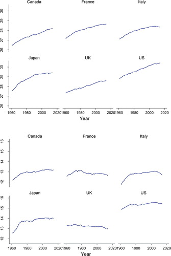
Several studies have pointed out the presence of measurement errors in CO₂ emission data (Wang et al. 2017; Quick and Marland 2019; Oda et al. 2019) and in GDP data (Targett 1989; Aruoba et al. 2016; Chang and Li 2018). In order to illustrate the applicability of the suggested wavelet denoising approach, we consider the long-run relation between CO₂ emissions (in metric tons) and real GDP in the seven advanced economies in the world (G7): Canada, France, Germany,¹⁰ Italy, Japan, the United Kingdom and the United States. The data is obtained from the World Development Indicators (WDI) database of the World Bank and spans over 1961–2014, that is 54 observations for each country. Figure 1 plots the two variables.

Fig. 1 Time series plots of real GDP and CO₂ emissions for G7 countries.

Prior to testing for cointegration, we must assess the integration properties of the two variables. We first check whether or not CO₂ emissions and real GDP series are integrated of order one, denoted I(1), or at least integrated of the same order. If they are, they may possibly share the same common stochastic trend component. We apply the Dickey–Fuller generalized least squares (DFGLS) t-test of Elliott, Rothenberg, and Stock (1996). This test is significantly more powerful than previous versions of the ADF test. We test the null hypothesis that the series is a random walk, possibly with drift, against the alternative that the series is stationary about a linear time trend. The results, reported in Appendix, indicate that CO₂ emissions and real GDP series are I(1) for all the six countries.

Table 4 reports the results of the Johansen test and the wavelet-based Johansen test. By applying the traditional Johansen test, the null hypothesis of no cointegration relationship is rejected for Canada at 5% and for the US at 10% significance level. The wavelet-based test, however, suggests no evidence of cointegration for the six countries.

Table 4 Johansen’s cointegration rank test for CO₂ emissions and real GDP for G7 countries.

		Raw		Wavelet-filtered
		Trace	Max	Trace	Max
Canada		16.83149	16.33953${}^{**}$	11.09735	10.80527
France		12.17422	12.07443	12.59538	12.15689
Italy		16.11574	11.1317	11.8465	7.644609
Japan		12.51058	10.50275	20.73	16.93427
UK		14.36162	8.777436	18.87543	15.42667
US		14.56135	13.67809${}^{*}$	12.13949	12.13227
Critical	5%	18.98116	15.73698	30.62131	25.47691
values	10%	16.59603	13.51135	26.69733	21.8588

Notes: The critical values are simulated for 54 observations (1961–2014), with 10,000 replications. The soft thresholding approach was applied for denoising the data and for generating critical values. The hypotheses to be tested are H0: r = 0; H1: r > 0 (Trace) and H0: r = 0; H1: r = 1 (Maximum Eigenvalue). The two hypotheses are basically the same since the two variables (n = 2) are both I(1), and there can be at most $n-1$ cointegrating relationships ($r)$. * and ** indicate rejections of the null hypothesis at 10% and 5% significance levels respectively.

6 Concluding remarks

This article investigates the effect of measurement errors on the performance of the Johansen (1988) cointegration likelihood ratio test. By employing Monte Carlo simulations, we find that empirical measurement errors result in over rejection of the true null hypothesis of no cointegration, and what is especially remarkable is that this bias increases as the sample size increases. As a remedy, a wavelet-based denoising transformation of the data is suggested using the Haar filter with MODWT. The statistical size and power of the Johansen test applied on raw and denoised data are computed for different DGPs by varying the parameters that determine the adjustment toward the equilibrium, the signal to noise ratio, and the sample sizes. The simulation results provide evidence that the denoising approach is effective with a statistical size of the wavelet-based Johansen test close to the nominal size. Most importantly, in contrast to Johansen’s test, the size of our wavelet test gets closer to the nominal size as the sample size increases, even for very noisy data.

Moreover, our wavelet-based Johansen test exhibits attractive properties in terms of statistical power. The power improves with the sample size, and the relative gain in power increases as the measurement error increases. The Haar filter combined with soft thresholding yields less distorted size, and there are no significant differences between hard and soft thresholding when it comes to statistical power. Based on our simulation results, we can recommend using wavelet-denoised data before testing for cointegration. We then applied the tests to examine the long-run equilibrium between CO₂ emissions and real GDP in the G7 countries. The traditional Johansen (1988) test provides evidence of an equilibrium relation for Canada and weak evidence for the US. However, our wavelet-based Johansen test suggests that these conclusions may be erroneous due to measurement errors that distort the size of the Johansen test and leads to over rejection of the null hypothesis of no cointegration.

Notes

¹ Consider the following regression model $y_i=\alpha +\beta {\tilde{x}}_i+u_i$, where $\tilde{x}$ is x observed with noise ω so that ${\tilde{x}}_i=x_i+{\omega }_i$. Replacing $x_i={\tilde{x}}_i-{\omega }_i$, the regression model becomes $y_i=\alpha +\beta x_i+v_i$ with $v_i=-\beta {\omega }_i+u_i$; then $\mathit{cov}(x_i,v_i)=E(x_i,v_i)$ $=E\left[({\tilde{x}}_i+{\omega }_i)(-\beta {\omega }_i+u_i)\right]=-\beta {\sigma }_{\omega }^2\ne 0$.

Since x_i is correlated with v_i, the OLS estimator is biased. $\widehat{\beta }\simeq \beta \left[\frac{{\sigma }_{\tilde{x}}^2}{{\sigma }_{\omega }^2+{\sigma }_{\tilde{x}}^2}\right]$ where $\frac{{\sigma }_{\tilde{x}}^2}{{\sigma }_{\omega }^2+{\sigma }_{\tilde{x}}^2}$ is between 0 and 1, which implies that $\left|\widehat{\beta }\right|$ is smaller than β. Measurement errors are thus biasing the OLS coefficient toward zero.

² See Hughes B., Random Walks and Random Environments, Vol. I, Sec. 2.1 (Oxford 1995).

³ Unlike Engle-Granger approach, it is possible to add restrictions to the cointegrating vectors; coefficients estimates are symmetrically distributed and median unbiased, even when errors are non-normally distributed (Gonzalo 1994).

⁴ The size is defined as the rejection frequency under the true null hypothesis while the power is defined as the rejection frequency of the false null hypothesis for size-adjusted cointegration tests.

⁵ One cannot rule out the possibility of non-classical measurement errors; there are cases where measurement errors might be correlated with the true variable (the signal), for example in the tails of the income distribution. For a thorough discussion of the effect of non-classical measurement errors, see Chen, Hong, and Tamer (2005).

⁶ For robustness checks, in addition to Haar wavelet, the Daubechies wavelet of length four, D(4) and the Daubechies least asymmetric wavelet of length eight, LA(8) were also applied in simulations. The compact support for these wavelets is in the interval [0, L – 1], where L denotes the wavelet length. Thus, Haar wavelet has compact support in interval [0, 1], the D(4) wavelet has compact support in the interval [0, 3], and the LA(8) wavelet has compact support in the interval [0, 7] (Percival and Walden 2000; Habimana 2018). The results are qualitatively similar across these three wavelets. Due to limited space, however, only Haar-based simulations are presented.

⁷ Terminology used by Jansson and Haldrup (2002), and Banerjee, Dolado, and Mestre (1998). Near zero ${\phi }_1$ values are chosen, since a powerful test is expected to distinguish near-non-cointegrated processes from non-cointegrated ones.

⁸ This is the case of “weak exogeneity” (Johansen 1992; Boswijk 1995; Urbain 2009). However, Hassler and Kuzin (2009) show that different values of ${\phi }_2$ leave the size and power of Johansen’s test essentially unaffected.

⁹ Compared to over-sized tests.

¹⁰ Germany was not included in the analysis because its CO₂ emissions series start late in 1991.

Appendix

Table A1 Critical values for Johansen cointegration test (5% level of significance, s = 0).

	Johansen (1988)’s		Wavelet-based Johansen		Wavelet-based Johansen
	test		test (Haar, soft)		test (Haar, hard)
T	Trace	Max.	Trace	Max.	Trace	Max.
30	20.399	16.974	32.44	26.941	29.687	25.017
50	19.356	16.088	30.954	25.602	28.093	23.657
100	18.859	15.614	29.185	24.25	26.448	22.553
200	18.462	15.378	28.587	23.855	27.233	22.764
500	18.294	15.059	28.223	23.472	27.051	22.624

Table A2 Unit root test.

	In levels		In first difference
	Real GDP	CO 2	ΔReal GDP	ΔCO2
Canada	–1.147	–0.964	–4.197***	–4.619***
France	–0.388	–1.053	–3.748**	–3.786***
Italy	–0.304	–0.313	–6.198***	–3.416**
Japan	–0.035	–1.002	–4.119***	–4.270***
UK	–2.747	–1.509	–4.774***	–4.135***
US	–1.303	–1.277	–4.592***	–4.812***

Notes: ** and *** indicate significance of the Elliott–Rothenberg–Stock DFGLS test statistic at the 5% and 1% level respectively. The optimal lag length is in parentheses and it is selected based on Schwert (1989) criterion. The null hypothesis is that the series is a random walk, possibly with drift, against the alternative that the series is stationary about a linear time trend.

References

- Antoniadis, A. 2007. “Wavelet Methods in Statistics: Some Recent Developments and Their Applications.” Statistics Surveys 1:16–55. doi: 10.1214/07-SS014.
- Aruoba, S. B., F. X. Diebold, J. Nalewaik, F. Schorfheide, and D. Song. 2016. “Improving GDP Measurement: A Measurement-Error Perspective.” Journal of Econometrics 191 (10):384–97. doi: 10.1016/j.jeconom.2015.12.009.
- Banerjee, A., J. Dolado, and R. Mestre. 1998. “Error-Correction Mechanism Tests for Cointegration in a Single-Equation Framework.” Journal of Time Series Analysis 19 (9):267–83. doi: 10.1111/1467-9892.00091.
- Boswijk, P. 1995. “Efficient Inference on Cointegration Parameters in Structural Error Correction Models.” Journal of Econometrics 69 (1):133–58. doi: 10.1016/0304-4076(94)01665-M.
- Chang, A. C., and P. Li. 2018. “Measurement Error in Macroeconomic Data and Economics Research: Data Revisions, Gross Domestic Product, and Gross Domestic Income.” Economic Inquiry 56 (9):1846–69. doi: 10.1111/ecin.12567.
- Chen, X., H. Hong, and E. Tamer. 2005. “Measurement Error Models with Auxiliary Data.” Review of Economic Studies 72 (10):343–66. doi: 10.1111/j.1467-937X.2005.00335.x.
- Cragg, J. G. 1994. “Making Good Inferences from Bad Data.” Canadian Journal of Economics 27 (4):776–800. doi: 10.2307/136183.
- Daubechies, I. 1992. Ten Lectures on Wavelets. CBMS-NSF Regional Conf. Series in Applied Mathematics. Philadelphia, PA: SIAM.
- Donoho, D. L., and I. M. Johnstone. 1994. “Ideal Spatial Adaptation by Wavelet Shrinkage.” Biometrika 81 (9):425–55. doi: 10.1093/biomet/81.3.425.
- Duffy, J. A., and D. F. Hendry. 2017. “The Impact of Integrated Measurement Errors on Modeling Long-Run Macroeconomic Time Series.” Econometric Reviews 36 (6–9):568–87. doi: 10.1080/07474938.2017.1307177.
- Elliott, G., T. Rothenberg, and J. H. Stock. 1996. “Efficient Tests for an Autoregressive Unit Root.” Econometrica 64 (4):813–36. doi: 10.2307/2171846.
- Engle, R. F., and C. W. J. Granger. 1987. “Co-Integration and Error Correction: Representation, Estimation and Testing.” Econometrica 55 (10):251–76. doi: 10.2307/1913236.
- Fischer, A. M. 1990. “Cointegration and I(0) Measurement Error Bias.” Economics Letters 34 (9):255–59. doi: 10.1016/0165-1765(90)90127-M.
- Gao, H. Y., and A. Bruce. 1997. “Waveshrink with Firm Shrinkage.” Statistica Sinica 7:855–74.
- Gençay, R., F. Selçuk, and B. Whitcher. 2002. An Introduction to Wavelets and Other Filtering Methods in Finance and Economics. San Diego, CA: Academic Press.
- Gonzalo, J. 1994. “Five Alternative Methods of Estimating Long-Run Equilibrium Relationships.” Journal of Econometrics 60 (1–2):203–33. doi: 10.1016/0304-4076(94)90044-2.
- Granger, C. W. J. 2009. “Developments in the Study of Cointegrated Economic Variables.” Oxford Bulletin of Economics and Statistics 48 (9):213–28. doi: 10.1111/j.1468-0084.1986.mp48003002.x.
- Granger, C. W. J., and P. Newbold. 1974. “Spurious Regressions in Econometrics.” Journal of Econometrics 2 (10):111–20.
- Haar, A. 1910. “Zur Theorie Der Orthogonalen Funktionensysteme.” Mathematische Annalen 69 (9):331–71. doi: 10.1007/BF01456326.
- Habimana, O. 2018. “Asymmetry and Multiscale Dynamics in Macroeconomic Time Series Analysis.” JIBS Dissertation Series No. 122.
- Habimana, O. 2019. “Wavelet Multiresolution Analysis of the Liquidity Effect and Monetary Neutrality.” Computational Economics 53 (1):85–110. doi: 10.1007/s10614-017-9725-1.
- Haldrup, N., A. Montanes, and A. Sanso. 2005. “Measurement Errors and Outliers in Seasonal Unit Root Testing.” Journal of Econometrics 127 (1):103–28. doi: 10.1016/j.jeconom.2004.06.005.
- Hamilton, J. D. 1994. Time Series Analysis, vol. 2. Princeton, NJ: Princeton University Press.
- Hassler, U., and V. Kuzin. 2009. “Cointegration Analysis under Measurement Errors.” Advances in Econometrics 24:131–50.
- Hong, H., S. K. Ahn, and S. Cho. 2016. “Analysis of Cointegrated Models with Measurement Errors.” Journal of Statistical Computation and Simulation 86 (9):623–39. doi: 10.1080/00949655.2015.1032289.
- Jansson, M., and N. Haldrup. 2002. “Regression Theory for Nearly Cointegrated Time Series.” Econometric Theory 18 (6):1309–35. doi: 10.1017/S0266466602186026.
- Johansen, S. 1988. “Statistical Analysis of Cointegration Vectors.” Journal of Economic Dynamics and Control 12 (2–3):231–54. doi: 10.1016/0165-1889(88)90041-3.
- Johansen, S. 1991. “Estimation and Hypothesis Testing of Cointegration Vectors in Gaussian Vector Autoregressive Models.” Econometrica 59 (6):1551–80. doi: 10.2307/2938278.
- Johansen, S. 1992. “Cointegration in Partial Systems and the Efficiency of Single-Equation Analysis.” Journal of Econometrics 52 (9):389–402. doi: 10.1016/0304-4076(92)90019-N.
- Johansen, S. 1996. Likelihood-Based Inference in Cointegrated Vector Autoregressive Models, 2nd ed. Oxford: Oxford University Press.
- Lütkepohl, H., P. Saikkonen, and C. Trenkler. 2001. “Maximum Eigenvalue versus Trace Tests for the Cointegrating Rank of a VAR Process.” The Econometrics Journal 4 (10):287–310. doi: 10.1111/1368-423X.00068.
- Månsson, K. 2012. “A Wavelet-Based Approach of Testing for Granger Causality in the Presence of GARCH Effects.” Communications in Statistics—Theory and Methods 41 (4):717–28. doi: 10.1080/03610926.2010.529535.
- Morgenstern, O. 1963. On the Accuracy of Economic Observations. Princeton, NJ: Princeton University Press.
- Nielsen, H. B. 2016. “The Co-Integrated Vector Autoregression with Errors-in-Variables.” Econometric Reviews 35 (10):169–200. doi: 10.1080/07474938.2013.806853.
- Oda, T., R. Bun, V. Kinakh, P. Topylko, M. Halushchak, G. Marland, T. Lauvaux, et al. 2019. “Errors and Uncertainties in a Gridded Carbon Dioxide Emissions Inventory.” Mitigation and Adaptation Strategies for Global Change 24 (6):1007–50. doi: 10.1007/s11027-019-09877-2.
- Pagan, A. 1984. “Econometric Issues in the Analysis of Regressions with Generated Regressors.” International Economic Review 25 (1):221–47. doi: 10.2307/2648877.
- Percival, D. B., and A. T. Walden. 2000. Wavelet Methods for Time Series Analysis. Cambridge, UK: Cambridge University Press.
- Quick, J. C., and E. Marland. 2019. “Systematic Error and Uncertain Carbon Dioxide Emissions from US Power Plants.” Journal of the Air & Waste Management Association 69 (5):646–58. doi: 10.1080/10962247.2019.1578702.
- Schwert, G. W. 1989. “Tests for Unit Roots: A Monte Carlo Investigation.” Journal of Business and Economic Statistics 7:147–60. doi: 10.2307/1391432.
- Targett, D. 1989. “UK GDP—Measurement Errors and Adjustments.” Omega 17 (4):345–53. doi: 10.1016/0305-0483(89)90048-0.
- Toda, H. Y. 1994. “Finite Sample Properties of Likelihood Ratio Tests for Cointegrating Ranks When Linear Trends Are Present.” The Review of Economics and Statistics 76 (1):66–79. doi: 10.2307/2109827.
- Urbain, J. P. 2009. “On Weak Exogeneity in Error Correction Models.” Oxford Bulletin of Economics and Statistics 54 (10):187–207. doi: 10.1111/j.1468-0084.1992.mp54002004.x.
- Wang, Y., G. Broquet, P. Ciais, F. Chevallier, F. Vogel, N. Kadygrov, L. Wu, Y. Yin, R. Wang, and S. Tao. 2017. “Estimation of Observation Errors for Large-Scale Atmospheric Inversion of CO2 Emissions from Fossil Fuel Combustion.” Tellus B: Chemical and Physical Meteorology 69 (1):1325723. doi: 10.1080/16000889.2017.1325723.
- Yule, U. 1926. “Why Do We Sometimes Get Nonsense-Correlations between Time Series?—A Study in Sampling and the Nature of Time Series.” Journal of the Royal Statistical Society 89 (1):1–63.