Parameter estimation of structural equation models with misclassification: The MC-SIMEX approach

Abstract

The random errors in the measurement process, called measurement error or misclassification, are inevitable and cause bias and inconsistent parameter estimates. Misclassification Simulation Extrapolation (MC-SIMEX) is a simulation based measurement error estimation method to obtain reduced parameter bias under misclassification. The main purpose of this study is an adaptation of MC-SIMEX method on Structural Equation Modeling (SEM). The effects of misclassification on the parameter estimates of a binary explanatory variables in SEM and the performance of MC-SIMEX method investigated with both Monte Carlo and an empirical study. According to the main results, finding the best extrapolant function is just as important as estimating the misclassification matrix although MC-SIMEX corrected a part of the bias.

Keywords:

• Structural equation models
• misclassification
• misclassification simulation extrapolation
• bias correction

1 Introduction

Traditionally, an assumption underlying statistical methods is that the variables of interest are observed. However, in practice, it is often impossible to measure or observe the variables of interest. Latent variables are defined as variables that are not observed (not measureable) but they can be estimated (through a statistical model) from other variables that are observed (manifest variables). Permanent income, intelligence, or socioeconomic status are common examples of typical latent variables. In the literature, latent variables are modeled through a factor analysis model. If, additionally, a structural model is present then the two parts is a Structural Equation Model (SEM), a very general statistical modeling technique in the social and behavioral sciences. SEM is often attributed to Jöreskog (1970), and for a more general introduction see Bollen (1989).

According to Wansbeek and Meijer (2001), there is a conceptual distinction between the latent variables concept and the notion of measuring variables with errors. Mismeasured (error-prone) explanatory variables, which is observed instead of true variables, cause biased and inconsistent parameter estimates. The statistical models for analyzing mismeasured data are called measurement error models or errors-in-variables model (Fuller 1987). The main aim of the measurement error models is to reduce bias. The Simulation-Extrapolation (SIMEX) method, introduced by Cook and Stefanski (1994), is considered as one of the most successful methods in the recent literature if the continuous explanatory variables are error-prone. Measurement error for binary variables means that observations has a probability to be misclassified. The SIMEX method was adjusted by Kuchenhoff, Mwalili, and Lesaffre (2006) to misclassified variables with the name Misclassification Simulation-Extrapolation (MC-SIMEX).

Lomax (1986) emphasized that for SEM models, although SEM incorporates a measurement model, the presence of measurement error is still problematic. The impact of measurement error on SEM was originally demonstrated by Fornell and Larcker (1981a, 1981b). As a consequence, methods to estimate SEM models with error-prone variables were proposed. As an example, Item Response Theory (IRT), unlike the classical additive measurement error definition, is a method that allows to use the conditional definition for measurement error (Fox and Glas 2003). Similarly, instrumental variables cannot be of use in solving the problems originating from measurement error, it just provides an improvement on the parameter estimates dependent on the instruments of sufficient quality and relevance, see e.g., Staiger and Stock (1994) for measurement errors and Hu (2008) for misclassification.

These methods can help to make “less-than-perfect measurement” and is generally considered that correcting for attenuation are both desirable and critical (Bedeian, Day, and Kelloway 1997). The MC-SIMEX method is a computation-based method for bias-correction and it compensates the lack of mathematical understanding of estimation bias. In the literature, Lawrence (2009) introduced the SIMEX procedure to SEM. He proposed the use of SIMEX when accounting for the estimation uncertainty and bias in a secondary estimation step where the estimated latent variables is used as an explanatory variable. Rutkowski and Zhou (2015) used the MC-SIMEX method for the estimation of single latent regression model on the 2006 Progress in International Reading Literacy Study (PIRLS) where the latent variable is IRT scores based on 91 items. In a first step they use IRT to estimate test scores which then is used as explanatory variable in a regression. This study basically demonstrated the success of MC-SIMEX. However, there is no study that exploring the performance of MC-SIMEX on SEM with misclassified categorical explanatory variable. Inspired from that, the main purpose of this study is an adaption of the MC-SIMEX method to the SEM. The performance of MC-SIMEX on SEM is important in terms of providing more reliable results from the applications as it is expected to give less biased estimates compared to the naive estimators.

According to the main results of paper, we first note that from the Monte Carlo study, as one expects increasing misclassification cause an increase in bias and mean square error of parameter estimations and MC-SIMEX fixes this partially. The empirical example also supports these findings. MC-SIMEX method could be considered as one of the successful measurement error model estimation techniques in SEM although estimating the misclassification matrix and finding better extrapolant function complicate the applicability of this method.

The paper is structured as follow: The next section, Section 2, demonstrates the SEM and MC-SIMEX methods. Then, the affects of misclassification error and the performance of MC-SIMEX are examined in Section 3 through Monte Carlo experiments. An empirical example based on the PIRLS data is in Section 4. Finally, Section 5 contains the conclusion and discussions.

2 Models and methods

In this section we first introduce the SEM model and then MC-SIMEX.

2.1 Structural equation models

In this section we summarize the Structural Equation Model, often abbreviated SEM. The SEM model structure is defined as to consist of two parts; the structural model with endogenous variables in the vector η as a function of exogenous variables ξ through the parameter matrices B and Γ, and the error ζ:(1) $$\eta =B\eta +\Gamma \xi +\zeta ,$$(1) and the measurement models, where Λ is matrices with factor loadings relating the latent variables η and ξ with the observed x and y, δ, and ϵ are errors in the measurement equations:$$x={\Lambda }_x\xi +\delta ,$$$$y={\Lambda }_y\eta +ϵ.$$

The structural model is the part that represents the thematic theory. For example, we can have that reading literacy depends on factors at home and at school. Factors at home can be parents education and how much the child reads outside school. Factors at school can be resources etc. Often there are not exact defined variables for reading literacy, how much the child reads outside of school etc. Instead there are many variables that reflects what we want to observe. In a survey questions can be asked about how often the child read books, how often they read comics, and how often newspapers. Then these three variables can be used in a factor analysis model for the purpose of modeling the latent variable Reading outside schools. Reading literacy can be measured by reading tests taken at school. Hence, there is a measurement model relating the variables we want to observe with the one we actually observe.

The estimation of a SEM model is usually done by maximum likelihood or by minimizing the distance between the observed covariance matrix of the variables, S and the model implied, $\Sigma (\theta )$. The likelihood is$$F_{ML}=-\hspace{0.17em}\text{log}\hspace{0.17em}(\Sigma (\theta ))-\text{tr}\left(S{\Sigma }^{-1}(\theta )\right)+\hspace{0.17em}\text{log}\hspace{0.17em}(S)+C$$where C is a constant that does not depend on the parameters or data. Expressions for the implied covariance matrix, $\Sigma (\theta )$, is shown in for example Bollen (1989, 325).

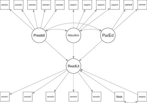
A convenient way to represent SEM models is the path diagram. In a path diagram boxes represents observed variables and circles latent variables. Then arrow shows relationships between the variables. An example of a path diagram is Fig. 1 which is the model used in the empirical section below. An excellent introductory text regarding SEM models is Bollen (1989).

Fig. 1 The estimated SEM model with variable labels.

2.2 Misclassification simulation-extrapolation

Consider a standard regression model in which the response variable Y and explanatory variable X are assumed truly observed. In empirical applications, a substitute or surrogate variable W is observed instead of the true X. The relationship between true X and its observation W represents with classical additive measurement error model $W=X+U$, where U is the measurement error which is distributed with mean zero and variance ${\sigma }_U^2$ and independent from X. The regression of Y on W are referred as naive estimator and the naive estimates are biased and inconsistent since the measurement error is ignored. This type of bias is called attenuation and the amount of attenuation is explained with the reliability ratio. For a simple linear regression model, the reliability ratio is $\lambda ={\sigma }_X^2/({\sigma }_X^2+{\sigma }_U^2)$ which is a real number in the range $[0,1]$, where ${\sigma }_X^2$ is the variance of X (Fuller 1987).

To explain MC-SIMEX, let say that this regression model has an binary explanatory variable,(2) $$Y={\beta }_{0,\mathit{true}}+{\beta }_{1,\mathit{true}}X+ϵ$$(2) where the parameters called true as we assume that both Y and X are truly observed. The measurement error concept explained above is for continuous explanatory variables. But, if X is a binary latent variable, the misclassification error definition arises instead of the classical additive measurement error. To describe the method for a misclassified latent explanatory variable, the misclassification matrix Π is defined by its components as below (Kuchenhoff, Mwalili, and Lesaffre 2006):$${\pi }_{ij}=P(W=i|X=j).$$

This definition corresponds a conditional probability that equals the probability of the observed value equal i when the true observation is j, which it is denoted π_ij . For a binary variable, Π is a 2 × 2 matrix:(3) $$\left[\begin{array}{cc}{\pi }_{00}& 1-{\pi }_{11}\\ 1-{\pi }_{00}& {\pi }_{11}\end{array}\right],$$(3) where π₀₀ and π₁₁ represent the probabilities of true observations. It means, the case of no misclassification corresponds to having $\Pi =I$. Based on Π, the naive model and its parameter estimates can be shown to be, see e.g., (Kuchenhoff, Mwalili, and Lesaffre 2006; Sevilimedu 2017):$$\begin{array}{c}E(Y|W)={\beta }_{0,\mathit{naive}}+{\beta }_{1,\mathit{naive}}W\\ {\beta }_{0,\mathit{naive}}={\beta }_{0,\mathit{true}}+{\beta }_{1,\mathit{true}}\frac{(1-{\pi }_{11}){\pi }_x}{{\pi }_{00}-\delta {\pi }_x}\\ {\beta }_{1,\mathit{naive}}={\beta }_{1,\mathit{true}}\frac{\delta (1-{\pi }_x){\pi }_x}{(1-{\pi }_{00}+\delta {\pi }_x)({\pi }_{00}-\delta {\pi }_x)}\end{array}$$ where δ is the determinant of Π matrix and π_x is the marginal probability $P(X=1)$.

Kuchenhoff, Mwalili, and Lesaffre (2006) adapted the SIMEX methodology and named it the Misclassification SIMEX (MC-SIMEX) to correct the naive estimator in the case of misclassification. Accordingly there are two steps: Simulation and extrapolation.

In the simulation step, a fixed grid of values ${\lambda }_1,\dots ,{\lambda }_m$ is defined and then we regenerate B sets of misclassified data for each λ_k ,$$W_{b,i}({\lambda }_k)=MC\left[{\Pi }^{{\lambda }_k}\right](W_i)$$where $i=1,\dots ,n;b=1,\dots ,B;k=1,\dots ,m$ and MC is the misclassification operation.¹ Also, ${\Pi }^{\lambda }$ equals to $E{\Lambda }^{\lambda }{E}^{-1}$ where E is the eigenvalues and Λ is the diagonal matrix of eigenvalues. It should be noted here, to calculate ${\Pi }^{\lambda }$, det(Π) should be larger than zero. As we have a binary latent variable, det($\Pi )={\pi }_{00}+{\pi }_{11}-1$ and the condition is fulfilled if ${\pi }_{00}>0.5$ and ${\pi }_{11}>0.5$.² Then, ${\widehat{\beta }}_{\mathit{naive}}$ estimations calculate as below for each λ_k ,$${\widehat{\beta }}_{\mathit{naive}}({\lambda }_k)=B^{-1}\sum _{b=1}^B{\widehat{\beta }}_{\mathit{naive}}\left[{(Y_i,W_{b,i}({\lambda }_k),Z_i)}_{i=1}^n\right];\hspace{1em}k=1,\dots ,m.$$

In the extrapolation step, the information of the ${\widehat{\beta }}_{\mathit{naive}}({\lambda }_k)$ averages corresponding to data with misclassification matrix ${\Pi }^{{\lambda }_k}$ are used in an extrapolant function $\mathcal{G}(\lambda ,\Gamma )$. Then, obtain estimator $\widehat{\Gamma }$ through the extrapolation function and $\lambda =-1$ point gives the MC-SIMEX estimates. More precisely, the extrapolant function can be the regression$${\widehat{\beta }}_{\mathit{naive}}\left({\lambda }_k\right)={\alpha }_0+{\alpha }_1(1+{\lambda }_k)+u_k.$$

As noted by e.g., Kuchenhoff, Mwalili, and Lesaffre (2006), a linear term is not always sufficient and often a quadratic term, ${(1+{\lambda }_k)}^2$, is added to the regression.

As the there is no closed form solution to the estimation problem of the parameters in the SEM model there are no analytical results regarding the relationship between the degree of misclassification and the bias induced by the misclassification. Hence, we rely on the MC-SIMEX approach to investigate this. This evolves to simulating samples for different values of λ through the λ distorted misclassification matrix, saving parameter estimates and the using the extrapolant function to adjust the parameter estimates.

3 Monte Carlo simulation

In this section, we will carry out a Monte Carlo simulation investigating small sample properties of the MC-SIMEX method applied to SEM models. We generate data accordingly to estimation results outlined in the empirical section below. More specifically, the Norwegian 2006 PIRLS round. The path diagram of the estimated model in which has three exogenous latent variables and one endogenous latent variable is displayed in Fig. 1. The number of items for the exogenous latent variables are 5, 4, and 2, respectively, while for the endogenous there are 5. Additional to the three exogenous explanatory latent variables, we included two explanatory dummy variables. One of them is sex and the other one is a background variable if the child spoke the test language before entering school. The language variable is assumed to be measured with error modeled by a misclassification matrix.

To clarify, we first generate data without misclassification, then we use misclassification matrix on the generated language variable to get a misclassified variable. This implies that we can estimate on data with and without misclassification and the two versions of MC-SIMEX (the linear and the quadratic models). Previous results indicate that the sample size is not important for the relative results between these four estimators, see e.g., Küchenhoff, Lederer, and Lesaffre (2007) and Nolte (2007), hence, we use the original sample size of N = 2, 857. The misclassification matrix is important and three of them will be used:(4) $${\Pi }_1=\left(\begin{array}{cc}0.977& 0.569\\ 0.022& 0.431\end{array}\right),{\Pi }_2=\left(\begin{array}{cc}0.85& 0.569\\ 0.15& 0.431\end{array}\right),{\Pi }_3=\left(\begin{array}{cc}0.977& 0.15\\ 0.022& 0.85\end{array}\right).$$(4)

The first matrix is estimated on the empirical data. The second one is obtained by increasing the misclassification of when the variable truly is zero, while the last one is obtained by reducing the misclassification when the variable truly is one. The number of replicates in the MC-SIMEX estimation method is 100 while the total number of replicates is 2,500. Preliminary investigations of the results indicate that it is mainly the parameter for the language variable that are effected and only those results are presented. We evaluate using bias and mean squared error (MSE) which are displayed between in Tables 1 to 3. First we note that the NAIVE estimator have larger bias and larger MSE compared to the all other estimators. Regarding both bias and MSE we can notice that the results differ substantially depending on which misclassification matrix that is used when generating the misclassification. As one can expect increasing misclassification, i.e., comparing ${\Pi }_2$ with ${\Pi }_1$, increase bias and MSE while decreasing it (comparing ${\Pi }_3$ with ${\Pi }_1$) decrease bias and MSE in general. The increased MSE for ${\Pi }_2$ compared to both ${\Pi }_1$ and ${\Pi }_3$ is due to larger bias, which is in turn due to lower probability for a correct classification. The exception is bias for β_SIMEXQ but it is reasonable to see this very low bias as pure luck as it is considerable lower than estimating using the variable without misclassification. For larger values of misclassification (${\Pi }_1$ and ${\Pi }_2$) the quadratic SIMEX is better in terms of MSE while for lower, ${\Pi }_3$ the linear is better. This is expected as when the misclassification is low, there is hardly any effect of λ and we get overfitting and poor fit for λ = 0 (which is outside the range used in estimation).

Table 1 Bias of parameter estimates.

	βNOME	βSIMEX	βSIMEXQ	βNAIV E
π1	−0.018	0.049	0.001	0.079
π2	−0.018	0.123	0.085	0.135
π3	−0.017	−0.003	−0.014	0.022

NOME denotes the bias of the estimates when using the variable without misclassification, SIMEX and SIMEX respectively denotes the linear MC-SIMEX and the Quadratic respectively, while NAIVE when estimating using the variable with misclassification. The rows corresponds to the three misclassification matrices.

Table 2 Bias of parameter estimates with random misclassification matrix.

	βNOME	βSIMEX	βSIMEXQ	βNAIV E
π1	−0.018	0.049	0.001	0.080
π2	−0.018	0.123	0.084	0.134
π3	−0.018	−0.004	−0.015	0.021

NOME denotes the bias of the estimates when using the variable without misclassification, SIMEX and SIMEX respectively denotes the linear MC-SIMEX and the Quadratic respectively, while NAIVE when estimating using the variable with misclassification. The rows corresponds to the three misclassification matrices. The misclassification matrices used are randomly drawn from the population misclassification matrices.

Table 3 Relative MSE of parameter estimates.

	βSIMEX	βSIMEXQ	βNAIV E
π1	4.645	1.691	10.507
π2	25.757	14.355	30.294
π3	0.716	1.149	1.349

SIMEX and SIMEX respectively denotes the relative mean squared error of the estimates when using the linear MC-SIMEX and the Quadratic respectively, while NAIVE when estimating using the variable with misclassification. The normalization is the mean squared error of the estimator without misclassification. The rows corresponds to the three misclassification matrices.

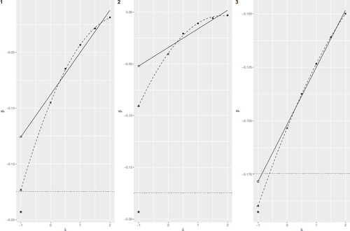
To get a better understanding of the results Fig. 2 shows a Monte Carlo version of the SIMEX plot. The two regression models are based on the average over all replicates. It seems like that the figures fairly well fit the data but as the SIMEX estimates are based on λ = 0 which is relatively far from the values of x used in the regression, even small departures yields bad SIMEX estimates. To complicate things, even the estimator based in correctly measured data is slightly biased and the size of the bias depends on the parameter value. Hence, what happens is that there are two effects. The first one is downward bias and then the failure to accurately capture the curvature of the SIMEX function which yields a small compensation. These two effects cancel out explaining why we have small bias and small MSE in certain cases.

Fig. 2 SIMEX figures for the three misclassification matrices based on Monte Carlo data. Square ($\square$) indicates the MC-SIMEX estimate using linear extrapolant function, triangle (Δ) using quadratic extrapolant function, cross (×) the naive, and star (*) without measurement error. The solid line is the SIMEX with linear extrapolant function and the dashed with quadratic. The horizontal dotted line marks the true value.

As the misclassification matrix is estimated, the simulation is also conducted in such a manner that for each replicate a misclassification matrix is randomly drawn using the binomial distribution with the entries of the misclassification matrix as population values. As seen in Tables 2 the bias is very similar and unaffected while for the mean squared error the results are mixed, see Table 4. For the misclassification matrix π₁ the mean squared error increase somewhat while decrease for π₂ and π₃. As a robustness check, limited Monte Carlo simulations has been conducted where the models have been changed somewhat. Overall, the results stays the same and, hence, the results are not reported.

Table 4 Relative MSE of parameter estimates with random misclassification matrix.

	βSIMEX	βSIMEXQ	βNAIV E
π1	4.816	1.732	10.769
π2	25.043	13.808	29.550
π3	0.686	1.126	1.254

SIMEX and SIMEX respectively denotes the relative mean squared error of the estimates when using the linear MC-SIMEX and the Quadratic respectively, while NAIVE when estimating using the variable with misclassification. The normalization is the mean squared error of the estimator without misclassification. The rows corresponds to the three misclassification matrices. The misclassification matrices used are randomly drawn from the population misclassification matrices.

4 Empirical example

The purpose of this section is to exemplify the above introduced methodology in an empirical relevant setting. The progress in international reading literacy study, PIRLS, has the purpose of assessing trends in reading achievement at the fourth grade. The main outcome variable is reading literacy which is measured by five items. There are a number of factors that influence reading literacy, see for example Elley (1994) for a discussion. Here we focus on preschool skills (5 items), reading out of school (4 items), and parents’ education (2 items). It is a well-known result that girls tend to perform better than boys, see e.g., Mullis et al. (2003), we include gender as an explanatory variable. There is also literature on the negative effects on reading literacy of children speaking another language at home than the language used in school, see e.g., Lesaux et al. (2006). In this spirit, we include whether or not the test language was spoken by the child prior to beginning school.

The PIRLS has four rounds, 2001, 2006, 2011, and 2016. In the 2001 round the test language question were asked to child whereas in the 2006 round it was asked to both the child and to the parents. We assume, as e.g., Rutkowski and Zhou (2015) does, that the parents answers correct while the child does not necessarily do that. With this setup we can estimate a model without and with misclassification for the 2006 round but only with misclassification for the 2001 round. We can use the MC-SIMEX methodology to adjust the 2001 estimates for the misclassification. To exemplify, we use data for Norway which consists of N = 2, 857 complete observations, i.e., 2,857 individuals that have no missing values at any of the used variables which implies that we can estimate the misclassification matrix as the parents answer is assumed to be correct. The estimated misclassification matrix is, with standard errors in italics below,(5) $$\Pi =\left(\begin{array}{cc}\underset{0.00270}{0.977}& \underset{0.00899}{0.569}\\ \underset{0.00912}{0.022}& \underset{0.0303}{0.431}\end{array}\right).$$(5)

The estimated model is shown in Fig. 1 with the variable names used in the 2006 study.³ The estimation results, i.e., parameter estimates and the z statistics, are shown in Table 5. The SEM models are estimated using the R package lavaan, (Rosseel 2012). The standard errors used to calculate the z statistics for the MC-SIMEX is bootstrapped with B = 399 bootstrap replicates. To account for the variability due to the estimation of the misclassification matrix, for each bootstrap replicate a misclassification matrix is drawn using the binomial distribution using the probabilities in the estimated misclassification matrix. As can be noted from the table the point estimates are very similar for all variables within each round except for the language variable. When introducing measurement error it get closer to zero, from about –0.175 to –0.137. Using MC-SIMEX the estimate is –0.182 which is very close to the estimate without measurement error. Adding a quadratic term in the MC-SIMEX regression yields a parameter estimate of –0.256 which is an overcompensated estimate compared to the results without misclassification. For the 2001 round the estimate with measurement error is –0.059 with MC-SIMEX estimate of –0.077. With the quadratic term included, the estimate is –0118 which then probably is an overestimate. It is also noteworthy that the z statistics are similar within each round, no matter if they are based on asymptotic theory or bootstrap.

Table 5 Estimation results for the structural parameters.

	${06}_h$	${06}_s$	${06}_{\mathit{SIMEX}}$	${06}_{\mathit{SIMEXQ}}$	${01}_s$	${01}_{\mathit{SIMEX}}$	${01}_{\mathit{SIMEXQ}}$
βPreskill	−0.272	−0.262	−0.264	−0.270	0.360	0.360	0.358
z	−15.668	−14.961	−15.558	−15.558	20.405	19.292	18.998
β RdoutSch	−0.055	−0.056	−0.055	−0.053	−0.098	−0.098	−0.095
z	−2.812	−2.812	−2.537	−2.360	−4.541	−4.033	−3.909
βParEd	0.404	0.413	0.410	0.396	0.401	0.401	0.402
z	20.938	21.370	20.088	18.568	18.418	17.934	18.193
βsex	−0.087	−0.092	−0.092	−0.090	−0.073	−0.073	−0.073
z	−5.254	−5.538	−5.239	−5.009	−4.306	−4.366	−4.346
βPreLan	−0.175	−0.137	−0.183	−0.254	−0.059	−0.074	−0.122
z	−10.699	−8.279	−7.303	−6.971	−3.499	−2.639	−2.825

h and s respectively denotes if the pre-language variable is answered from parents (the home questionnaire) or by student. SIMEX denotes the linear extrapolant model and SIMEXQ the model with quadratic extrapolant. Lastly, 06 denotes the 2006 round and 01 the 2001. The z-statistics are based on 399 bootstrap replicates where the misclassification matrix is randomly drawn from binomial distribution.

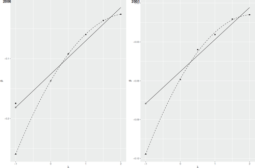
An informative figure is Fig. 3 where λ is on the x-axes and β on the y. This kind of figures can be used to decide upon the functional relationship between λ and the parameter estimates. The solid line is the SIMEX using a linear term and the dashed with quadratic, both fitted to the solid dots. We can see that the quadratic model fits the data better than the linear although the fit is not perfect. It is of interest to compare the fitted values for λ = 0 with the naive estimator and the estimate using the variable without measurement error. The linear and quadratic SIMEX estimates are on the corresponding lines and denoted $\square$ and Δ respectively while the naive is ×. For the 2006 data, we also have the estimate without measurement error marked with *. The naive estimate is substantially attenuated zero the other while there is also a substantial difference between the two SIMEX estimates with the quadratic well below the linear. The 2006 estimate without measurement error is very close to the linear estimate and that supports the findings that the linear extrapolant function has better performance to correcting bias.

Fig. 3 SIMEX figure. 2006 on the left and 2001 on the right. Square ($\square$) indicates the MC-SIMEX estimate using linear extrapolant function, triangle (Δ) using quadratic extrapolant function, cross (×) the naive, and for 2006, star (*) without measurement error. The solid line is the SIMEX with linear extrapolant function and the dashed with quadratic.

5 Conlusion

In this paper, the effects of misclassification of a explanatory variable in the SEM framework is investigated using Monte Carlo methods. The effects are evaluated through bias and MSE. The performance of the MC-SIMEX method, which is one of the successful misclassification estimation method was examined with both Monte Carlo simulations and an empirical example. The Norwegian 2001 and 2006 PIRLS data sets used as an empirical example.

In the Monte Carlo studies, the effects of three misclassification matrices whereof one of them was estimated using the empirical data, were analyzed for the naive and the MC-SIMEX method. Results demonstrates that ignoring misclassification error cause large bias and MSE even when the misclassification probabilities are small. As one can expect, increasing misclassification increase bias and MSE. According to both the Monte Carlo and the empirical study, the MC-SIMEX method has good performance regarding reducing bias. The amount of correction varies according to the extrapolant function used. We compare the linear and the quadratic function and the linear extrapolant function gave less bias. But the results depends heavily on the misclassification matrix. This is contrary to Kuchenhoff, Mwalili, and Lesaffre (2006) where the extrapolant function well characterizes the relationship.

Additionally, as the misclassification matrix has major impact on the results, the estimation of this matrix is an important issue. For experimental data, repeated measures, additional information (like in our empirical example), or known distribution information can be used to estimate the misclassification matrix. Otherwise, estimation methods from previous studies can be used, see e.g., Cohen (1960), Fuller (1987), Veierød and Laake (2001), and Nakagawa (2018).

To sum up, this study shows how misclassification in binary exogenous variables affects the parameter estimates in SEM models and how the MC-SIMEX method can be used to remediate these averse problems. For future research, different model structures and different extrapolant functions (i.e., log-linear function) could be examined. Improving the estimation of misclassification matrix and choosing the extrapolant function will increase the applicability of this method in a variety of fields.

Acknowledgments

This research was presented at the International Conference on Trends and Perspectives in Linear Statistical Inference (LinStat 2020), Bedlewo, Poland, 30 August–3 September, 2021. We also gratefully acknowledge comments and suggestions from the reviewers.

Disclosure statement

The authors declare no conflicts of interest.

Additional information

Funding

Sahika Gokmen is supported by the International Postdoctoral Research Scholarship Program of The Scientific and Technological Research Council of Turkey (TUBITAK BIDEB 2219).

Notes

1 The misclassification operator basically is that for a given observed value of W_i new values are drawn using the relevant probabilities in the matrix ${\Pi }^{{\lambda }_k}$.

2 For the case of three or more categories see Kuchenhoff, Mwalili, and Lesaffre (2006)

3 Foy and Kennedy (2008) has a variable list that gives the corresponding variable names for the 2001 round.

Appendix

In this appendix we explicitly state the parameters matrices and variables (with the names used in the PIRLS codebook) used in the estimation. The latent variables are $\xi ={\left[\text{Preskill},\text{RdoutSch},\text{ParEd}\right]}^T$ and $\eta =\left[\text{ReadLit}\right]$. The exogenous indicators are divided into three sets:$$x_1={\left[\text{asbhaib}1,\text{asbhaib}2,\text{asbhaib}3,\text{asbhaib}4,\text{asbhaib}5\right]}^T,$$$$x_2={\left[\text{asbgrto}1,\text{asbgrto}2,\text{asbgrto}3,\text{asbgrto}4\right]}^T,$$$$x_3={\left[\text{asbhledf},\text{asbhledm}\right]}^T$$and the endogenous indicators are$$y={\left[\text{asrrea}01,\text{asrrea}02,\text{asrrea}03,\text{asrrea}04,\text{asrrea}05\right]}^T.$$

The measurement models are$$\begin{array}{c}\left[\begin{array}{c}{x}_1\\ x_2\\ x_3\end{array}\right]=\left[\begin{array}{ccc}{\lambda }_1& 0& 0\\ ⋮& ⋮& \\ {\lambda }_5& 0& ⋮\\ 0& {\lambda }_6& \\ & & \\ ⋮& {\lambda }_9& 0\\ & 0& {\lambda }_{10}\\ 0& 0& {\lambda }_{11}\end{array}\right]\left[\begin{array}{c}{\xi }_1\\ {\xi }_2\\ {\xi }_3\end{array}\right]+\left[\begin{array}{c}{\delta }_1\\ ⋮\\ {\delta }_{11}\end{array}\right]\\ E\xi {\xi }^T=\left[\begin{array}{ccc}1& {\varphi }_{12}& {\varphi }_{13}\\ {\varphi }_{21}& 1& {\varphi }_{23}\\ {\varphi }_{31}& {\varphi }_{32}& 1\end{array}\right]\\ y=\left[\begin{array}{c}{\lambda }_{y1}\\ ⋮\\ {\lambda }_{y5}\end{array}\right]\eta +\left[\begin{array}{c}{ϵ}_1\\ ⋮\\ {ϵ}_5\end{array}\right]\end{array}$$

The covariance matrices of δ and ϵ are diagonal. The structural model is$$\eta ={\beta }_1{\zeta }_1+{\beta }_2{\zeta }_2+{\beta }_3{\zeta }_3+{\beta }_{\mathit{itsex}}\text{itsex}+{\beta }_{\mathit{asbglng}1}\text{asbglng}1+\zeta$$

References

- Bedeian, A. G., D. V. Day, and E. K. Kelloway. 1997. “Correcting for Measurement Error Attenuation in Structural Equation Models: Some Important Reminders.” Educational and Psychological Measurement 57 (5):785–799. doi: 10.1177/0013164497057005004.
- Bollen, K. A. 1989. Structural Equations with Latent Variables. New York: Wiley.
- Cohen, A. C. 1960. “Misclassified Data from a Binomial Population.” Technometrics 2 (1):109–113. doi: 10.1080/00401706.1960.10489884.
- Cook, J. R., and L. A. Stefanski. 1994. “Simulation-Extrapolation Estimation in Parametric Measurement Error Models.” Journal of the American Statistical Association 89 (428):1314–1328. doi: 10.1080/01621459.1994.10476871.
- Elley, W. B. 1994. The IEA Study of Reading Literacy: Achievement and Instruction in Thirty-Two School Systems. Oxford, UK: Pergamon Press.
- Fornell, C., and D. F. Larcker. 1981a. “Evaluating Structural Equation Models with Unobservable Variables and Measurement Error,” Journal of Marketing Research 18 (1):39–50.
- Fornell, C., and D. F. Larcker. 1981b. “Structural Equation Models with Unobservable Variables and Measurement Error: Algebra and Statistics.” Journal of Marketing Research 18 (3):382–388. doi: 10.2307/3150980.
- Fox, J.-P., and C. A. Glas. 2003. “Bayesian Modeling of Measurement Error in Predictor Variables Using Item Response Theory.” Psychometrika 68 (2):169–191. doi: 10.1007/BF02294796.
- Foy, P., and A. Kennedy. 2008. PIRLS 2006 User Guide Supplement 1 for the International Database. TIMSS & PIRLS International Study Center, Lynch School of Education, Boston College.
- Fuller, W. A. 1987. Measurement Error Models. New York: Wiley.
- Hu, Y. 2008. “Identification and Estimation of Nonlinear Models with Misclassification Error using Instrumental Variables: A General Solution.” Journal of Econometrics 144 (1):27– 61. doi: 10.1016/j.jeconom.2007.12.001.
- Jöreskog, K. G. 1970. “A General Method for Estimating a Linear Structural Equation System.” ETS Research Bulletin Series 1970 (2):i–41. doi: 10.1002/j.2333-8504.1970.tb00783.x.
- Küchenhoff, H., W. Lederer, and E. Lesaffre. 2007. “Asymptotic Variance Estimation for the Misclassification Simex.” Computational Statistics & Data Analysis 51 (12):6197–6211. doi: 10.1016/j.csda.2006.12.045.
- Kuchenhoff, H., S. M. Mwalili, and E. Lesaffre. 2006. “A General Method for Dealing with Misclassification in Regression: The Misclassification Simex.” Biometrics 62 (1):85–96. doi: 10.1111/j.1541-0420.2005.00396.x.
- Lawrence, C. N. 2009. “Accounting for the” Known Unknowns”: Incorporating Uncertainty in Second-Stage Estimation.” Texas A&M International University Working Paper.
- Lesaux, N. K., K. Koda, L. S. Siegel, and T. Shanahan. 2006. “Developing Literacy in Second-Language Learners.” In Developing Literacy in Second-Language Learners: Report of the National Literacy Panel on Language-Minority Children and Youth, edited by D. August and T. Shanahan. Lawrence Erlbaum Associates, Mahwah, NJ.
- Lomax, R. G. 1986. “The Effect of Measurement Error in Structural Equation Modeling.” The Journal of Experimental Education 54 (3):157–162. doi: 10.1080/00220973.1986.10806415.
- Mullis, I. V. S., M. O. Martin, E. J. Gonzalez, and A. M. Kennedy. 2003. PIRLS 2001 International Report: IEA’s Study of Reading Literacy Achievement in Primary Schools. Chestnut Hill, MA: Boston College.
- Nakagawa, T. 2018. “Estimating the Probabilities of Misclassification using cv when the Dimension and the Sample Sizes are Large.” Hiroshima Mathematical Journal 48 (3):373–411. doi: 10.32917/hmj/1544238034.
- Nolte, S. 2007. “The Multiplicative Simulation Extrapolation Approach.” Center for Quantitative Methods and Survey Research, University of Konstanz, Working Paper.
- Rosseel, Y. 2012. “lavaan: An R Package for Structural Equation Modeling.” Journal of Statistical Software 48 (2):1–36.
- Rutkowski, L., and Y. Zhou. 2015. “Correcting Measurement Error in Latent Regression Covariates via the mc-simex Method.” Journal of Educational Measurement 52 (4):359–375. doi: 10.1111/jedm.12090.
- Sevilimedu, V. 2017. Application of the Misclassification Simulation Extrapolation (Mc- Simex) Procedure to Log-Logistic Accelerated Failure Time (Aft) Models in Survival Analysis. PhD thesis.
- Staiger, D. O., and J. H. Stock. 1994. “Instrumental Variables Regression with Weak Instruments.” Working Paper 151, National Bureau of Economic Research, Cambridge.
- Veierød, M. B., and P. Laake. 2001. “Exposure Misclassification: Bias in Category Specific Poisson Regression Coefficients.” Statistics in Medicine 20 (5):771–784. doi: 10.1002/sim.712.
- Wansbeek, T., and E. Meijer. 2001. “Measurement Error and Latent Variables.” In A Companion to Theoretical Econometrics, edited by B. H. Baltagi, 162–179. Oxford, UK: Basil Blackwell.