Regularized estimation of the Mahalanobis distance based on modified Cholesky decomposition

Abstract

Estimating inverse covariance matrix is an essential part of many statistical methods. This paper proposes a regularized estimator for the inverse covariance matrix. Modified Cholesky decomposition (MCD) is utilized to construct positive definite estimators. Instead of directly regularizing the inverse covariance matrix itself, we impose regularization on the Cholesky factor. The estimated inverse covariance matrix is used to build Mahalanobis distance (MD). The proposed method is evaluated by detecting outliers through simulations and empirical studies.

Keywords:

• Modified Cholesky decomposition
• Mahalanobis distance
• regularization
• smoothing
• outlier detection

1 Introduction

Estimating the covariance matrix and its inverse is a fundamental question in statistics due to their broad use in different applications including portfolio allocation and the analysis of gene expression data. Very recently, Bodnar, Bodnar, and Parolya (2022) reviewed the mostly used shrinkage estimators for covariance and precision matrices. They additionally provided the application in portfolio theory where the weights of optimal portfolios are usually determined as functions of the mean vector and covariance matrix. One important usage of covariance matrix is in Mahalanobis distance (MD) that has been used in many research areas with different applications, such as assessing multivariate normality (Hoffelder 2019), classification and discriminant analysis (Mardia 1977), multivariate calibration (De Maesschalck, Jouan-Rimbaud, and Massart 2000) and construction of multivariate process control charts (Cabana and Lillo 2021), etc. One of the predominant applications of MD is outlier detection. The effect of outliers has been noticed decades ago (Barnett 1978) and the usage of MD for outlier detection was introduced ever since. MD is a measurement on the distance between two observations. Taking into account of the covariance for the observations gives MD advantages comparing to other distance measures, for example, Euclidean distance. See Peng et al. (2021) and the references therein for a comprehensive review about various empirical applications of MD to measure the distance of observations. MD was proposed by Mahalanobis (1930) and defined as follows:$$D\left({\mathit{y}}_i,\mathit{\mu },\mathbf{\Sigma }\right)=\left({\mathit{y}}_i-\mathit{\mu }\right)\prime {\mathbf{\Sigma }}^{-1}\left({\mathit{y}}_i-\mathit{\mu }\right),$$where $(·)\prime$ is the transpose of a vector or matrix, the vector ${\mathit{y}}_i,i=1,\dots ,n$, is the ith observation with the mean vector $\mathit{\mu }$ and covariance matrix $\mathbf{\Sigma }$. When the covariance matrix $\mathbf{\Sigma }$ is unknown, it has been noticed that the sampling properties of any estimated MD will depend upon the estimator of ${\mathbf{\Sigma }}^{-1}$ (see Dai and Holgersson 2018, for example). However, obtaining a stable and efficient estimator of the inverse covariance matrix has faced some challenges. Among others, when the sample size (n) is smaller than the number of variables (p), one classical estimator—sample covariance matrix becomes singular. This context are usually referred as high-dimensional dataset, i.e., the ratio $p/n=c>1$. In recent years, there exists a growing literature on developing new types of MD which are based on various techniques, including ridge-type estimators (Holgersson and Karlsson 2012), minimum diagonal product estimator (Ro et al. 2015) and factor model (Dai 2020) as well as MD for complex random vectors (Dai and Liang 2021). Furthermore, the needing of preserving the positive definiteness of covariance matrices has raised another difficulty when modeling covariance structures since the positive definiteness requirement for the covariance matrix may impose complicated non-linear constraints on the parameters (Kim and Zimmerman 2012).

For high-dimensional data, we often face the problem of information redundancy such as extra variables that are not important to reveal the causality for the studied problem. Regularization is the class of methods which aims to modify maximum likelihood estimator (MLE) to give reasonable answers in unstable situations (Bickel and Li 2006). The obtained results will preserve information in the dataset while the regularized model will be further simplified and easy to get a deeper insight into a dataset. Usually, there are two perspectives about the regularization in literature when estimating large covariance matrix. One direction is to regularize the covariance matrix itself. Rothman, Levina, and Zhu (2009) proposed a general threshold on regularization of the sample covariance matrix in high dimensions. Cai and Yuan (2012) suggested a blocked threshold on estimation of a covariance matrix. The estimator is constructed by dividing the sample covariance matrix into blocks and then simultaneously estimating the entries in a block by threshold. The other direction is to do the regularization through appropriate matrix factorization of a covariance matrix. Instead of directly regularizing the covariance matrix, regularization can be put on the factor matrices. One factorization which has been widely used is the modified Cholesky decomposition (MCD). Pourahmadi (1999, 2000) proposed a unique, completely unconstrained and interpret able reparameterization of a covariance matrix based on MCD. Huang et al. (2006) showed that shrinkage is very useful in providing a more stable estimate of a covariance matrix, especially when the dimension p is high. Bickel and Levina (2008) showed that banding the Cholesky factor can produce a consistent estimator in the operator norm under weak conditions on the covariance matrix. Tai (2009) proposed a penalized likelihood method for producing a statistically efficient estimator of a covariance matrix by introducing both shrinkage and smoothing on the Cholesky factor. The proposed regularization scheme was motivated by two observations of the Cholesky factor. First, the Cholesky factor is nearly sparsity condition that is likely to have many off-diagonal elements that are zero or close to zero. Second, there is usually continuity among neighboring elements of the Cholesky factor which is typical for covariance matrices of longitudinal data. Taking into account the smoothness can help to provide more efficient covariance matrix estimates.

In this paper, we adopt the idea of Tai (2009) and propose a new type of MD estimator which is based on regularized estimation of inverse covariance matrix. Besides guaranteeing the positive definiteness property of the covariance matrix, the connection of the covariance matrix and the least square regression lights up the utility of the regression related techniques to solve the issues of high-dimensional and singularity problems. Based on our conducted studies, the proposed estimator of the MD outperforms the classical MD and other benchmark methods on detecting outliers for both low and high-dimensional data. The computational procedure has been additionally implemented in R under “seamless R and C++ integration Rcpp” (Eddelbuettel et al. 2011).

The rest of the paper is organized as follows. In Section 2 we have a brief introduction of MCD method. The corresponding penalized likelihood functions of different penalties and the choice of tuning parameters are given in Section 3. In Section 4, we conduct a simulation study to compare MCD-based MD with the classical MD. Both the classical context n > p and the high-dimensional context p > n are studied. Section 5 is dedicated to the empirical study follows by concluding remarks in Section 6.

2 Modified Cholesky decomposition

In this section, we introduce the modified Cholesky decomposition. Without loss of generality, we assume $\mathit{Y}=({\mathit{y}}_1,{\mathit{y}}_2,\dots ,{\mathit{y}}_n)\sim N(\mathbf{0},\mathbf{\Sigma },{\mathit{I}}_n)$, i.e., matrix Y consists of n independent random vectors with length p and the covariance matrix $\mathbf{\Sigma }$ of ${\mathit{y}}_i$. Pourahmadi (1999, 2000) developed a parameterization of $\Sigma$ called modified Cholesky decomposition (MCD), i.e., there exists a unique lower triangular matrix $\mathit{T}$ with ones on the main diagonal and a unique diagonal matrix $\mathit{D}$ such that(1) $$\mathit{T}\mathbf{\Sigma }\mathit{T}\prime =\mathit{D},$$(1) where$$\mathit{T}=\left(\begin{array}{ccccc}1& 0& 0& \cdots & 0\\ -{\varphi }_{21}& 1& 0& \cdots & 0\\ -{\varphi }_{31}& {\varphi }_{32}& 1& \cdots & 0\\ ⋮& ⋮& \ddots & \ddots & ⋮\\ -{\varphi }_{p1}& -{\varphi }_{p2}& \cdots & -{\varphi }_{p(p-1)}& 1\end{array}\right)\mathrm{ }\text{and}\mathrm{ }\mathit{D}=\left(\begin{array}{cccc}{\sigma }_1^2& 0& \cdots & 0\\ 0& {\sigma }_2^2& \cdots & 0\\ ⋮& ⋮& \ddots & ⋮\\ 0& 0& \cdots & {\sigma }_p^2\end{array}\right).$$

Thus, the inverse covariance matrix ${\mathbf{\Sigma }}^{-1}=\mathit{T}\prime {\mathit{D}}^{-1}\mathit{T}$.

Based on Eq. (1)(1) $$\mathit{T}\mathbf{\Sigma }\mathit{T}\prime =\mathit{D},$$(1) and the property that normality is preserved under linear transformations, we have(3) $$\mathit{TY}=\mathit{E},\hspace{1em}\mathit{E}\sim N(\mathbf{0},\mathit{D},{\mathit{I}}_n),$$(3) which turns out that Eq. (3)(3) $$\mathit{TY}=\mathit{E},\hspace{1em}\mathit{E}\sim N(\mathbf{0},\mathit{D},{\mathit{I}}_n),$$(3) can be represented as the following linear model:(4) $${\mathit{y}}_t=\sum _{k=1}^{t-1}{\varphi }_{tk}{\mathit{y}}_k+{\mathit{e}}_t,\hspace{1em}{\mathit{e}}_t\sim N(\mathbf{0},{\sigma }_t^2{\mathit{I}}_n),\hspace{1em}t=2,\dots ,p,$$(4) where the elements of T, ${\varphi }_{tk}$, can be presented as the coefficients of the linear model with ${\mathit{y}}_t$ as the dependent variable and ${\mathit{y}}_1,{\mathit{y}}_2,\dots ,{\mathit{y}}_{t-1}$ as the independent variables. Observing Eq. (3)(3) $$\mathit{TY}=\mathit{E},\hspace{1em}\mathit{E}\sim N(\mathbf{0},\mathit{D},{\mathit{I}}_n),$$(3) has been split into p independent simple linear regression models and the MLE of the unknown parameters in (4) are actually ordinary least square (OLS) estimators. Thus, MCD provides an alternative MLE estimation procedure of $\mathbf{\Sigma }$ through a sequential regression scheme. The regression formulation gives a possibility of performing regularized estimation that combines both shrinkage and smoothing to matrix T as we shall present in Section 3. Based on MCD, the regularized estimation of $\mathbf{\Sigma }$ becomes $\widehat{\mathbf{\Sigma }}=\widehat{\mathit{T}}\widehat{\mathit{D}}{\widehat{\mathit{T}\prime }}^{-1}$, which preserves the positive definiteness of $\widehat{\mathbf{\Sigma }}$. At the same time, the regularization takes into account about the sparsity of the covariance matrix and dependency among the longitudinal type of data. So the information redundancy can be avoided.

3 Regularized estimation of the inverse covariance matrix

In this section, we introduce the implementation of the shrinkage and smoothing parameters on the decomposed component T and its elements $(-{\varphi }_{tj})$ in (1). Let λ_sk and λ_sm be the penalty parameters where “sk” means shrinkage and “sm” means smoothing respectively, we define the penalized likelihood functions in the next subsection.

3.1 Design of penalties and penalized likelihood

Equation (4)(4) $${\mathit{y}}_t=\sum _{k=1}^{t-1}{\varphi }_{tk}{\mathit{y}}_k+{\mathit{e}}_t,\hspace{1em}{\mathit{e}}_t\sim N(\mathbf{0},{\sigma }_t^2{\mathit{I}}_n),\hspace{1em}t=2,\dots ,p,$$(4) shows that the linear least square predictor of ${\mathit{y}}_t,{\widehat{\mathit{y}}}_t$, can be estimated based on its predecessors ${\mathit{y}}_{t-1},\dots ,{\mathit{y}}_1$ and ${\mathit{\epsilon }}_t={\mathit{y}}_t-{\widehat{\mathit{y}}}_t$ be its prediction error with variance ${\sigma }_t^2=\mathrm{var}({\epsilon }_{it})$, $i=1,\dots ,n$. Like the mean, this linear regression scheme gives possibilities to the estimation of covariance matrix and its inverse. Thus, we can utilize the shrinkage penalty that is usually imposed on the linear regression further on to the covariance matrix and its inverse. The shrinkage penalty on the likelihood function of the component of $\mathbf{\Sigma }$ is given as follows:(5) $${\lambda }_{sk}\sum _{t=2}^p\sum _{j=1}^{t-1}{\left|{\varphi }_{tj}\right|}^2,$$(5) which is also known as L₂ penalty. The L₂ penalty shrinks the estimates of ${\varphi }_{tj}$’s toward to zero and helps to produce more stable estimates. When ${\lambda }_{sk}=0$, the minimization of the penalized log-likelihood degenerates back to the classical MLE. Huang et al. (2006) considered a statistically efficient estimator based on the penalized normal likelihood with an L₂ penalty:(6) $$-2\mathcal{l}(\Sigma ,\mathit{Y})+{\lambda }_{sk}\sum _{t=2}^p\sum _{j=1}^{t-1}{\left|{\varphi }_{tj}\right|}^2=\sum _{t=1}^p\left(\mathrm{}n\hspace{0.17em}\text{log}\hspace{0.17em}{\sigma }_t^2+\sum _{i=1}^n{\mathit{\epsilon }}_{it}^2/{\sigma }_t^2\mathrm{}\right)+{\lambda }_{sk}\sum _{t=2}^p\sum _{j=1}^{t-1}{\left|{\varphi }_{tj}\right|}^2,$$(6) where ${\epsilon }_{i1}=y_{i1}$ and ${\epsilon }_{it}=y_{it}-{\sum }_{j=1}^{t-1}{y}_{ij}{\varphi }_{tj}$ for $t=2,\dots ,p$. The first part of (6) is the classical log-likelihood function. In our case, it is given as follows,(7) $$-2\mathcal{l}(\Sigma ,\mathit{Y})=\sum _{t=1}^p\left\{n\hspace{0.17em}\text{log}\hspace{0.17em}{\sigma }_t^2+\sum _{i=1}^n\frac{{(y_{it}-\sum _{j=1}^{t-1}{y}_{ij}{\varphi }_{tj})}^2}{{\sigma }_t^2}\right\}.$$(7)

The minimization of the penalized log-likelihood (6) with regards to σ_t and ${\varphi }_{tj}$ are given as follows, for $t=2,\dots ,p$,(8) $${\widehat{\sigma }}_t^2=n^{-1}\sum _{i=1}^n{\left(y_{it}-\sum _{j=1}^{t-1}{y}_{ij}{\widehat{\varphi }}_{tj}\right)}^2,$$(8) (9) $${\widehat{\varphi }}_{t(t)}={\left({\mathit{H}}_t+{\lambda }_{sk}{\mathit{I}}_t\right)}^{-1}{g}_t,$$(9) where (t) stands the first t – 1 columns of the Cholesky factor $\mathit{T},{\mathit{H}}_t$ is the cross moments of the first t – 1 periods of original dataset and can be expressed as ${\mathit{H}}_t=({\sum }_{t=1}^n{y}_{i(t)}y{\prime }_{i(t)})/{\widehat{\sigma }}_t^2,g_t=({\sum }_{t=1}^n{y}_{it}y{\prime }_{i(t)})/{\widehat{\sigma }}_t^2$ and ${\mathit{I}}_t$ is an identity matrix with $(t-1)$ dimensions. Additionally, the first element ${\widehat{\sigma }}_1^2$ is given as ${\widehat{\sigma }}_1^2={\sum }_{i=1}^n{y}_{i1}^2/n$. The estimators of T and D, which are denoted as ${\widehat{\mathit{T}}}_{sk}$ and ${\widehat{\mathit{D}}}_{sk}$, can be obtained using ${\widehat{\sigma }}_t^2$ and ${\widehat{\varphi }}_{t(t)}$ in (8) and (9), which are estimated iteratively until the estimators converge to a certain criterion.

Tai (2009) observed that one drawback of the shrinkage approach is that it ignores possible continuity among neighboring entries of the matrix T, which is a typical feature for covariance matrices of longitudinal data. Smoothing is a technique that connects the current observation to the previous observation by a simple functional form. The advantages of using smoothing are mainly twofold. Firstly, the function of smoothing is simple to implement, this feature will add minor computational burden to the estimating procedure, especially when the dataset has relatively high volume of observations and variables. Secondly, smoothing penalty can distinguish the meaningful signals from noises by using a different form of smoothing functions. The results only depend on a limited amount of previous observations which also reduces the complication of estimation. Here we implement the differencing along the sub-diagonal of the Cholesky factor and use smoothing spline as the smoothing penalty for the likelihood function:(10) $${\lambda }_{sm}\sum _{t=2}^{p-2}\sum _{j=1}^{t-1}{({\Delta }_{\mathit{diag}}^2{\varphi }_{t+2,t+2-j})}^2,$$(10) where ${\Delta }_{\mathit{diag}}^2{\varphi }_{t+2,t+2-j}=({\varphi }_{t+2,t+2-j}-{\varphi }_{t+1,t+1-j})-({\varphi }_{t+1,t+1-j}-{\varphi }_{t,t-j})$ is the second order difference in the lower triangle matrix T. In terms of the regression formulation of covariance matrices in (3), a smoothing function given in (10) is bidirectional operation which imposes smoothing across different regressions. Combining both shrinkage and smoothing in (5) and (10), the penalized log-likelihood function is defined as follows,(11) $$-2\mathcal{l}(\Sigma ,\mathit{Y})+{\lambda }_{sk}\sum _{t=2}^p\sum _{j=1}^{t-1}{\left|{\varphi }_{tj}\right|}^2+{\lambda }_{sm}\sum _{t=2}^{p-2}\sum _{j=1}^{t-1}{({\Delta }_{\mathit{diag}}^2{\varphi }_{t+2,t+2-j})}^2,$$(11) where $-2\mathcal{l}(\Sigma ,\mathit{Y})$ is presented in (7). The estimators of T and D, which are denoted as ${\widehat{\mathit{T}}}_{\mathit{skm}}$ and ${\widehat{\mathit{D}}}_{\mathit{skm}}$, can be obtained numerically.

Following the same idea of (8) and (9), we get the corresponding estimators of ${\widehat{\sigma }}_t^2$ and ${\widehat{\varphi }}_t$ as follows,(12) $${\widehat{\sigma }}_t^2=n^{-1}\sum _{i=1}^n{\left(y_{it}-\sum _{j=1}^{t-1}{y}_{ij}{\widehat{\varphi }}_{tj}\right)}^2,$$(12) (13) $${\widehat{\varphi }}_{t(t)}={\left({\mathit{H}}_t+{\lambda }_{sk}{\mathit{I}}_t+{\lambda }_{sm}{\mathit{E}}_t^{\prime }{\mathit{E}}_t\right)}^{-1}{g}_t.$$(13)

Here $H_t=\mathrm{diag}({\sigma }_{t+1}^{-2}{\sum }_{i=1}^n{y}_{i1}^2,{\sigma }_{t+2}^{-2}{\sum }_{i=1}^n{y}_{i2}^2,\dots ,{\sigma }_n^{-2}{\sum }_{i=1}^n{y}_{i,n-t}^2)$ is an $(n-t)\times (n-t)$ diagonal matrix and g_t is given as follows,$$g_t={\left(\mathrm{}{\sigma }_{t+1}^{-2}\sum _{i=1}^n{y}_{i1}\left(\mathrm{}{y}_{i,t+1}-\sum _{j=2}^t{y}_{ij}{\varphi }_{t+1,j}\mathrm{}\right),\dots ,{\sigma }_n^{-2}\sum _{i=1}^n{y}_{i,n-t}\left(\mathrm{}{y}_{i,n}-\sum _{\begin{array}{c}1\le j\le p-1\\ j\ne p-t\end{array}}{y}_{ij}{\varphi }_{nj}\mathrm{}\right)\mathrm{}\right)}^{\prime }.$$

Set ${\sum }_{t=2}^p{\sum }_{j=1}^{t-1}{\varphi }_{tj}^2={\sum }_{t=1}^{p-1}{\mathit{\gamma }}_t^{\prime }{\mathit{\gamma }}_t$ and ${\mathit{E}}_t,t=1,\dots ,p-3$, is the $(p-2-t)\times (p-t)$ matrix representation of the operator of the second order differencing ${\Delta }_{\text{diag}\mathrm{ }}^2$ such that ${\sum }_{j=1}^{t-1}{({\Delta }_{\text{diag}\mathrm{ }}^2{\varphi }_{t+2,t+2-j})}^2={\mathit{\gamma }}_t^{\prime }{\mathit{E}}_t^{\prime }{\mathit{E}}_t{\mathit{\gamma }}_t$. The algorithm of the MCD is given in Algorithm 1.

Algorithm 1 The algorithm of MCD (Tai 2009)

Initialize $\left\{{\mathit{\sigma }}_t^{2(1)},t=1,\dots ,p\right\}$ and $\left\{{\mathit{\gamma }}_t^{(1)},t=1,\dots ,p-1\right\}$

if n > p then

use maximum likelihood estimation as ${\mathit{\sigma }}_t^{2(1)},{\mathit{\gamma }}_t^{(1)}$

else if $n\le p$ then

use L₂ penalized likelihood estimate as ${\mathit{\sigma }}_t^{2(1)},{\mathit{\gamma }}_t^{(1)}$

end if

set $\mathit{tol}={10}^{-5}$

for i = 1 to 10⁴ do

(1) ${\mathit{\gamma }}_t^{(i+1)}={({\mathit{H}}_t^{(i)}+{\lambda }_{sh}{\mathit{I}}_t+{\lambda }_{sm}{\mathit{E}}_t^{\prime }{\mathit{E}}_t)}^{-1}{g}_t^{(i)}$

(2) ${\mathit{\sigma }}_t^{2(i+1)}=n^{-1}{\sum }_{i=1}^n{(y_{it}-{\sum }_{j=1}^{t-1}{y}_{ij}{\varphi }_{tj}^{(i+1)})}^2$

if min($|{\mathit{\sigma }}_t^{2(i+1)}-{\mathit{\sigma }}_t^{2(i)}|,|{\mathit{\gamma }}_t^{(i+1)}-{\mathit{\gamma }}_t^{(i)}|)\ge \mathit{tol}$ then

 Repeat (1) and (2)

else

 ${\mathit{\gamma }}_t^{(i+1)}={\mathit{\gamma }}_t^{(i)}$

 ${\mathit{\sigma }}_t^{2(i+1)}={\mathit{\sigma }}_t^{2(i)}$

end if

end for

return ${\mathit{\gamma }}_t^{(i+1)}$ and ${\mathit{\sigma }}_t^{2(i+1)}$

Denote ${\widehat{\mathbf{\Sigma }}}_{\mathit{skm}}^{-1}=\widehat{\mathit{T}}{\prime }_{\mathit{skm}}{\widehat{\mathit{D}}}_{\mathit{skm}}^{-1}{\widehat{\mathit{T}}}_{\mathit{skm}}$ as the estimated inverse covariance matrix which is based on penalized likelihood function (11). We obtain the following regularized estimator of the MD:(14) $${\widehat{D}}_{\mathit{skm}}={\mathit{x}}_i^{\prime }{\widehat{\mathbf{\Sigma }}}_{\mathit{skm}}^{-1}{\mathit{x}}_i,i=1,\dots ,n,$$(14) where ${\mathit{x}}_i=({\mathit{y}}_i-\overline{\mathit{y}})$ is the centered data of ${\mathit{y}}_i$ and $\overline{\mathit{y}}$ is the sample mean vector. The selection of the tuning parameters λ_sk and λ_sm in (11), will be discussed in the next subsection.

3.2 Selection of tuning parameters

Concerning the choice of the tuning parameters λ_sk and λ_sm , we use K-fold cross-validation (CV) which was suggested by Tai (2009). The procedure starts with randomly splitting the dataset into K folds of the same size. For each time we use K – 1 folds as a training data to estimate the model parameters and the rest one fold as a testing data to validation. This process will be repeated K times in order to find out the optimal values of the tuning parameters. Let ${\widehat{\mathbf{\Sigma }}}_{-k}$ and ${\widehat{\mathbf{\Sigma }}}_{-k}^{-1}$ be the estimators of the covariance matrix and its inverse which are based on the training data in the kth replication, $1\le k\le K$. The optimal values of tuning parameters are chosen by$$({\widehat{\lambda }}_{sk},{\widehat{\lambda }}_{sm})=\underset{{\lambda }_{sk},{\lambda }_{sm}}{\arg \min }\frac{1}{K}\sum _{k=1}^K\left(n_k\hspace{0.17em}\text{log}\hspace{0.17em}\left|{\widehat{\Sigma }}_{-k}\right|+\sum _{i\in \mathit{testing}}{\mathit{y}}_i^{\prime }{\widehat{\Sigma }}_{-k}^{-1}{\mathit{y}}_i\right),$$where n_k is the sample size of the testing data. The minimization is done through the grid-searching for each combination of the values of λ_sk and λ_sm , while ${\lambda }_{sm}=0$ corresponds to the case of only using the shrinkage penalty. In this paper, we set K = 5 as 5-fold cross-validation which is an optimal balancing between the estimation accuracy and computational feasibility (Arlot and Celisse 2010).

4 Simulations

In this section, we implement the simulation study. Contaminated datasets are simulated with different fractions of outliers (q), dimensions (p) and sample sizes (n). Several methods are used as the benchmarks and the results of outlier detection are compared to show the performance of MCD based MD. We consider two scenarios for the dimension of the datasets. One is when the sample size n is larger than the dimension of variables p. For this case, the methods we use include the robust high breakdown point methods (minimum covariance determinant estimator (MCDE), orthogonalized Gnanadesikan–Kettenring (OGK), minimum volume ellipsoid (MVE) and Stahel–Donoho estimator (SDE)) together with the MCD based MD (MCD). The other scenario is when the sample size n is less than or equal to the dimension of variables p. For this case, the high breakdown point methods are not valid anymore. So we show the performance of MCD under the datasets that have different dimensions and sample sizes for the $n\le p$ cases.

The datasets are simulated from a Normal distribution $N(\mathit{0},\mathbf{\Sigma })$ where the correlation matrix is given as$$\mathbf{\Sigma }=\left(\begin{array}{ccccc}1& \rho & {\rho }^2& \dots & {\rho }^{n-1}\\ \rho & 1& \rho & \dots & {\rho }^{n-2}\\ ⋮& ⋮& ⋮& \ddots & ⋮\\ {\rho }^{n-1}& {\rho }^{n-2}& {\rho }^{n-3}& \dots & 1\end{array}\right),$$i.e., $\mathbf{\Sigma }$ that follows a Toeplitz structure with $\rho =0.7$. The contaminated datasets have several choices on the fractions for outliers $q\in \{0.05,0.1,0.2,0.3\}$, i.e., $q=0.05$ implies 5% of the observations are outliers. We randomly choose the observations from the datasets based on the fraction of outliers q. Then 3 times interquartile range is added to the chosen observations so that these observations are artificially converted into outliers. For each dataset, several combinations of dimensions p and sample sizes n are applied: the values of n and p are chosen from the set {10, 30, 50, 70, 100}. For each of these cases we generate 200 datasets, perform the outlier detection with each of the considered methods. One observation is considered as an outlier if its distance value is larger than 95th percentile across all the observations. As a result, the indices of the chosen observations will be used later for the evaluations about the different methods. All of the methods are evaluated by the following two measures:

• FP – Median non-outlier error rate: the median percentage of non-outliers that were classified as outliers—false positives or swamped non-outliers.

• FN – Median outlier error rate: the median percentage of outliers that were not identified—false negatives or masked outliers.

The results show that MCD outperforms across all the scenarios of outlier fraction on outlier detection. When $q\in \{0.05,0.1\}$, the FP of MCD is remained on 0% for most of the cases. As n increases to 100, in Table 2, the FP of MCD increases to 5%. The FNs of MCD are higher than the FPs of MCD in Tables 1–2 but keep at the level between 5% and 6.7%. While q increases, FNs of MCD remains at the same level but FPs of MCD various between 5% and 10%. Both FNs and FPs are stable for most of the cases.

Table 1 FP and FN for fraction of outliers q = 0.05.

Dimension	Error	SDE	MCDE	MVE	OGK	MCD
50 × 10	FP	1.0000	1.0000	1.0000	1.0000	0.0000
50 × 10	FN	0.9681	0.9362	0.9681	0.9468	0.0638
50 × 30	FP	1.0000	1.0000	1.0000	1.0000	0.1667
50 × 30	FN	0.9894	0.9681	0.9787	0.9362	0.0532
100 × 30	FP	1.0000	1.0000	1.0000	1.0000	0.0000
100 × 30	FN	0.9789	0.9842	0.9789	0.9474	0.0526
100 × 50	FP	0.9000	0.9000	0.9000	0.8000	0.0000
100 × 50	FN	0.9947	0.9947	0.9947	0.8895	0.0526

Table 2 FP and FN for fraction of outliers q = 0.1.

Dimension	Error	SDE	MCDE	MVE	OGK	MCD
50 × 10	FP	1.0000	1.0000	1.0000	1.0000	0.0000
50 × 10	FN	0.9778	0.9556	0.9556	0.9333	0.0667
50 × 30	FP	1.0000	1.0000	1.0000	1.0000	0.0000
50 × 30	FN	0.9889	0.9889	0.9889	0.8778	0.0667
100 × 30	FP	1.0000	1.0000	1.0000	0.8000	0.0500
100 × 30	FN	0.9722	0.9611	0.9667	0.8444	0.0500
100 × 50	FP	1.0000	1.0000	1.0000	0.8000	0.0500
100 × 50	FN	0.9944	0.9944	1.0000	0.7833	0.0500

When $p\ge n$, FNs are relatively steady with regard to different values of q. The values of FN is changing between 5.1% and 7.5% regardless the values of q, p, n. FPs are affected by the value of q that the increasing of q will increase the values of FP.

It is also noticeable that the ratio of dimension and sample size p/n may have contributed to the increase in both FPs and FNs. For example, the highest value in FP of MCD is found for the case $q=0.05$ in Table 1 when the ratio $p/n=0.6$. The same happens for case q = 0.2 in Table 3, there the FP of MCD is 10% for the 50 × 30 case. Some values of MCD decrease as the value of q increases. This happens mainly for the FP cases with a lower value of p/n. In this case, the value of p/n plays a crucial role on the performance of MCD based MD especially when p/n is approaching to 1 from both left and right hand side (Table 4). One example can be found in Table 5, as the p/n reaches 1, the FP value increases to 10% again. For most cases, the different values of q would not change too much on the results when the values of p/n are relatively small—e.g., less than 0.5. MCD works fine without being affected much by the amount of the outliers. The performance of the proposed method is connected to the correspondingly underlying idea with regard to an outlier. Our data-driven method keeps as many observations as possible in the dataset and filter out the contaminated observations. However the benchmark methods often tend to consider one observation as an outlier and remove it as long as the observation is lying slightly far away from the rest. This enlarges the scope of the potential outliers. These methods guarantees that the observations left are robust enough to be used for analysis. On the other hand, these methods filter out too many observations that can be considered as a loss of information. The method we proposed can find a balance between the classical methods that may miss several outliers and the benchmark methods that may remove more observations than the practical needing.

Table 3 FP and FN for fraction of outliers q = 0.2.

Dimension	Error	SDE	MCDE	MVE	OGK	MCD
50 × 10	FP	1.0000	1.0000	1.0000	0.9000	0.1000
50 × 10	FN	0.9750	0.9500	0.9750	0.8500	0.0500
50 × 30	FP	1.0000	1.0000	1.0000	0.8000	0.1000
50 × 30	FN	1.0000	0.9750	1.0000	0.7750	0.0500
100 × 30	FP	1.0000	1.0000	1.0000	0.8000	0.0500
100 × 30	FN	0.9875	0.9750	0.9875	0.7750	0.0500
100 × 50	FP	1.0000	1.0000	1.0000	0.7000	0.0500
100 × 50	FN	1.0000	1.0000	1.0000	0.7000	0.0500

Table 4 FP and FN for fraction of outliers q = 0.3.

Dimension	Error	SDE	MCDE	MVE	OGK	MCD
50 × 10	FP	0.9333	0.9333	1.0000	0.8667	0.0667
50 × 10	FN	0.9143	0.9429	0.9714	0.8857	0.0571
50 × 30	FP	1.0000	1.0000	1.0000	0.8667	0.0667
50 × 30	FN	1.0000	0.9714	1.0000	0.8857	0.0571
100 × 30	FP	1.0000	1.0000	1.0000	0.9333	0.0333
100 × 30	FN	0.9857	0.9857	0.9857	0.9286	0.0571
100 × 50	FP	1.0000	1.0000	1.0000	0.9000	0.0333
100 × 50	FN	1.0000	1.0000	1.0000	0.9000	0.0571

Table 5 FP and FN for fraction of outliers q $\in$ {0.05, 0.10, 0.20, 0.30}.

Dimension	Error	q = 0.05	q = 0.10	q = 0.20	q = 0.30
30 × 30	FP	0.0500	0.0714	0.0714	0.0450
30 × 30	FN	0.0576	0.0536	0.0536	0.0579
50 × 50	FP	0.0000	0.0000	0.0000	0.1000
50 × 50	FN	0.0667	0.00667	0.0750	0.0500
50 × 100	FP	0.0000	0.0000	0.0000	0.0000
50 × 100	FN	0.0638	0.0638	0.0714	0.0714
70 × 100	FP	0.0476	0.0909	0.0909	0.0586
70 × 100	FN	0.0612	0.0508	0.0508	0.0565

5 Empirical study

We apply our methods with three real-world data. The MCD based MD and the classical MD are calculated to measure the difference among the observations for each dataset. A distance is considered as outliers if it exceeds the 95% quantile of all the distances. Note the datasets here are chosen with a higher ratio value of p/n rather than the purely high numbers in n or p since the simulation section shows that the ratio of p/n affects the performance of MCD based MD more than the values of n or p.

The Leppik dataset records baseline seizure data (Base, computed as the logarithm of a quarter of the number of baseline seizure counts in the 8-week period preceding the trial), treatment (0 for placebo, 1 for drug), the interaction between treatment and baseline seizure, the logarithm of age and post-randomization clinic visit. The observation number 21 (patient number 207) is outstanding as an outlier comparing to the rest of the observations. Pardo and Hobza (2014) discussed the possible outliers and pointed out that observation number 21 (patient number 207) is an outlier because both the baseline and post-treatment counts are much higher than those of other patients. The result is the same to our detection with MCD based MD.

The ramus data were originally given by Elston and Grizzle (1962) and subsequently analyzed by Rao (1987), among others. Ramus height has been measured in millimeters, for each of a group of 20 boys at 8, 8.5, 9, and 9.5 years old. MCD based MD detects the observation number 4, 12 and 17 as the outlier. This result achieves a similar conclusion as the analysis given in Pan, Fang, and Fang (2002).

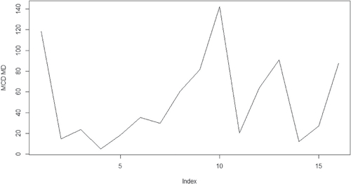
The third dataset, dental, was first considered by Potthoff and Roy (1964). Dental measurements were made on 11 girls and 16 boys at the ages of 8, 10, 12, and 14. Each measurement is the distance, in millimeters, from the center of the pituitary to the pterygomaxillary fissure. We split this dataset into two groups based on the gender. By doing so, we increase the ratio value of p/n that affects the performance of MCD based MD drastically in the simulation study. The MCD based MD identifies the individual number 10 in the girl group and individuals number 10 and 13 in the boy group as the extreme observations while the analysis in Pan, Fang, and Fang (2002) and von Rosen (1993) consider observations number 10 in the girl group and observations number 4, 10, and 13 in the boy group as outliers. The conclusions are very close between our results and previous research.

The calculated distances with regard to the above datasets are given in the Figs. 1–4 where x-axis is for the index for the observations, y-axis is for the values for the MCD based MDs. There one can see clearly that the outliers are outstanding comparing to the rest of the observations. The other methods such as the classical MD could only detect observation number 13 in the boy group as outliers across all the three datasets. This part of the results will not be presented in the paper.

Fig. 1 The index plot for MCD MDs for Leppik dataset.

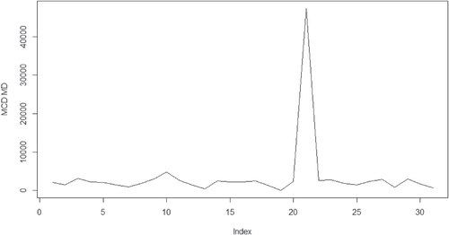
Fig. 2 The index plot for MCD MDs for the ramus dataset.

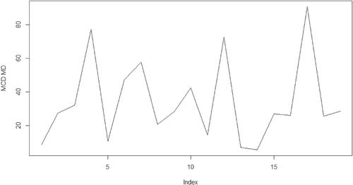
Fig. 3 The index plot for MCD MDs for the girl group dental dataset.

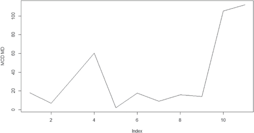
Fig. 4 The index plot for MCD MDs for the boy group dental dataset.

6 Concluding remarks

This paper concerns the MCD-based regularized estimator of MD. Using the regularized estimation of the inverse covariance matrix through shrinkage and smoothing penalties (Tai 2009), we investigate a new solution on detecting outliers and propose two new regularized estimators of MD. In spite of the availability of other estimators of MD for outlier detection, our approach contributes with the statistically efficient estimators of the inverse covariance matrix and yields a better performance via the simulation study. Particularly, the proposed estimated MD remains well behaved in high-dimensional data. Hence, our approach should provide a useful tool in identifying outliers of large longitudinal data.

The proposed approach is based on MCD method which relies on the order of variables. Natural ordering is typical for longitudinal data. When the situation arises that the variables do not have a natural ordering among themselves, the procedures derived in this paper can also be similarly obtained by for example addressing the variable order issue in the MCD method (Kang and Deng 2020a, 2020b). We hope to communicate the relevant results in a future correspondence.

Acknowledgments

Deliang Dai acknowledges the warm hospitality of Department of Mathematics at The university of Manchester where this work was initiated, during a visit funded by Linnaeus University. Authors are grateful to the referees for their detailed review and helpful suggestions which has resulted in significant improvement of this manuscript.

References

- Arlot, S., and A. Celisse. 2010. “A Survey of Cross-Validation Procedures for Model Selection.” Statistics Surveys 4:40–79. doi: 10.1214/09-SS054.
- Barnett, V. 1978. “Outliers in Statistical Data.” Technical report.
- Bickel, P. J., and E. Levina. 2008. “Covariance Regularization by Thresholding.” The Annals of Statistics 36:2577–604. doi: 10.1214/08-AOS600.
- Bickel, P. J., and B. Li. 2006. “Regularization in Statistics.” Test 15:271–344. doi: 10.1007/BF02607055.
- Bodnar, O., T. Bodnar, and N. Parolya. 2022. “Recent Advances in Shrinkage-based High-Dimensional Inference.” Journal of Multivariate Analysis 188:104826. 50th Anniversary Jubilee Edition. doi: 10.1016/j.jmva.2021.104826.
- Cabana, E., and R. E. Lillo. 2021. “Robust Multivariate Control Chart based on Shrinkage for Individual Observations.” Journal of Quality Technology 1–26. doi: 10.1080/00224065.2021.1930617.
- Cai, T. T., and M. Yuan. 2012. “Adaptive Covariance Matrix Estimation through Block Thresholding.” The Annals of Statistics 40:2014–42. doi: 10.1214/12-AOS999.
- Dai, D. 2020. “Mahalanobis Distances on Factor Model based Estimation.” Econometrics 8:10. doi: 10.3390/econometrics8010010.
- Dai, D., and T. Holgersson. 2018. “High-Dimensional CLTs for Individual Mahalanobis Distances.” In Trends and Perspectives in Linear Statistical Inference, edited by M. Tez and D. von Rosen, 57–68. Cham: Springer.
- Dai, D., and Y. Liang. 2021. “High-Dimensional Mahalanobis Distances of Complex Random Vectors.” Mathematics 9:1877. doi: 10.3390/math9161877.
- De Maesschalck, R., D. Jouan-Rimbaud, and D. L. Massart. 2000. “The Mahalanobis Distance.” Chemometrics and Intelligent Laboratory Systems 50:1–18. doi: 10.1016/S0169-7439(99)00047-7.
- Eddelbuettel, D., R. François, J. Allaire, K. Ushey, Q. Kou, N. Russel, J. Chambers, and D. Bates. 2011. “Rcpp: Seamless r and c++ integration.” Journal of Statistical Software 40:1–18.
- Elston, R., and J. E. Grizzle. 1962. “Estimation of Time-Response Curves and their Confidence Bands.” Biometrics 18 (2):148–59. doi: 10.2307/2527453.
- Hoffelder, T. 2019. “Equivalence Analyses of Dissolution Profiles with the Mahalanobis Distance.” Biometrical Journal 61 (5):1120–37. doi: 10.1002/bimj.201700257.
- Holgersson, T., and P. Karlsson. 2012. “Three Estimators of the Mahalanobis Distance in High-Dimensional Data.” Journal of Applied Statistics 39:2713–20. doi: 10.1080/02664763.2012.725464.
- Huang, J. Z., N. Liu, M. Pourahmadi, and L. Liu. 2006. “Covariance Matrix Selection and Estimation via Penalised Normal Likelihood.” Biometrika 93:85–98. doi: 10.1093/biomet/93.1.85.
- Kang, X., and X. Deng. 2020a. “An Improved Modified Cholesky Decomposition Approach for Precision Matrix Estimation.” Journal of Statistical Computation and Simulation 90:443–64. doi: 10.1080/00949655.2019.1687701.
- Kang, X., and X. Deng. 2020b. “On Variable Ordination of Cholesky-based Estimation for a Sparse Covariance Matrix.” Canadian Journal of Statistics 49 (2):283–310. doi: 10.1002/cjs.11564.
- Kim, C., and D. L. Zimmerman. 2012. “Unconstrained Models for the Covariance Structure of Multivariate Longitudinal Data.” Journal of Multivariate Analysis 107:104–118. doi: 10.1016/j.jmva.2012.01.004.
- Mahalanobis, P. 1930. “On Tests and Measures of Group Divergence.” Journal and Proceedings of Asiatic Society of Bengal 26:541–88.
- Mardia, K. 1977. “Mahalanobis Distances and Angles.” Multivariate Analysis IV 495–511.
- Pan, J.-X., K.-t. Fang, and K.-T. Fang. 2002. Growth Curve Models and Statistical Diagnostics. New York: Springer.
- Pardo, M. d. C., and T. Hobza. 2014. “Outlier Detection Method in GEEs.” Biometrical Journal 56 (5):838–50. doi: 10.1002/bimj.201300149.
- Peng, Z., L. Cheng, Q. Yao, and H. Zhou. 2021. “Mahalanobis-Taguchi System: A Systematic Review from Theory to Application.” Journal of Control and Decision 9 (2):139–151. doi: 10.1080/23307706.2021.1929525.
- Potthoff, R. F., and S. Roy. 1964. “A Generalized Multivariate Analysis of Variance Model Useful Especially for Growth Curve Problems.” Biometrika, 51 (3–4):313–26. doi: 10.1093/biomet/51.3-4.313.
- Pourahmadi, M. 1999. “Joint Mean-Covariance Models with Applications to Longitudinal Data: Unconstrained Parameterisation.” Biometrika 86:677–90. doi: 10.1093/biomet/86.3.677.
- Pourahmadi, M. 2000. “Maximum Likelihood Estimation of Generalised Linear Models for Multivariate Normal Covariance Matrix.” Biometrika 87:425–35. doi: 10.1093/biomet/87.2.425.
- Rao, C. R. 1987. “Prediction of Future Observations in Growth Curve Models.” Statistical Science 2 (4):434–47.
- Ro, K., C. Zou, Z. Wang, and G. Yin. 2015. “Outlier Detection for High-dimensional Data.” Biometrika 102:589–99. doi: 10.1093/biomet/asv021.
- Rothman, A. J., E. Levina, and J. Zhu. 2009. “Generalized Thresholding of Large Covariance Matrices.” Journal of the American Statistical Association 104:177–86. doi: 10.1198/jasa.2009.0101.
- Tai, W. 2009. “Regularized Estimation of Covariance Matrices for Longitudinal Data through Smoothing and Shrinkage.” PhD thesis, Columbia University.
- von Rosen, D. 1993. “Uniqueness Conditions for Maximum Likelihood Estimators in a Multivariate Linear Model.” Journal of Statistical Planning and Inference 36 (2–3):269–75. doi: 10.1016/0378-3758(93)90129-T.