Applications of a new loss and cost-based process capability index to electronic industries

Abstract

In this article, we propose a new process capability index called ${\mathcal{C}}_{\mathit{pmc}}^{\prime }$ which is based on asymmetric loss function (linear exponential) and tolerance cost function for a normal process which provides a tailored way of incorporating the loss and tolerance cost in capability analysis. Next, we estimate the proposed PCI ${\mathcal{C}}_{\mathit{pmc}}^{\prime }$ when the process follows the normal distribution using six classical methods of estimation and we compare the performance of the considered methods of estimation in terms of their mean squared errors through simulation study. Besides, five bootstrap methods are employed for constructing the confidence intervals for the index ${\mathcal{C}}_{\mathit{pmc}}^{\prime }$. The performance of the bootstrap confidence intervals (BCIs) are compared in terms of average width and coverage probabilities using Monte Carlo simulation. Finally, for illustrating the effectiveness of the proposed index and methods of estimation and BCIs, two real data sets from electronic industries are re-analyzed.

Keywords:

• Bootstrap confidence intervals
• classical methods of estimation
• cost function
• loss function
• process capability index

1 Introduction

In almost all manufacturing industries, processes are frequently assessed by adopting process capability indices (PCIs) which provide a numerical measure on whether a monitored process is capable of achieving the quality requirement pre-set by the customers. This statistical tool has received great attention in the quality control and statistical literature as it has been found very useful in decision making and enhancing efforts in process performance. For greater insight into classical capability indices, readers may refer to the works of: Juran (1974), Kane (1986), Chan, Cheng, and Spiring (1988), and Pearn, Kotz, and Johnson (1992). It is noteworthy that classical capability indices were developed by taking into account the assumption of normal probability model with process mean ε and process standard deviation Ϛ.

It dates back to 1974 when Juran (1974) first introduced the PCI denoted by C_p and is defined as (1.1) $${\mathcal{C}}_p=\frac{\mathcal{U}-\mathcal{L}}{6\varsigma }$$(1.1) where $\mathcal{U}$ and $\mathcal{L}$ are the upper and the lower specification limits. However, there are some limitations of ${\mathcal{C}}_p$. One such limitation is that it does not consider process mean. The second limitation is its inability to capture the variation when the process is not centered at the target value. In order to overcome these limitations, several indices were developed wherein variations from the target value are considered while measuring the capability of a particular process. One such index was developed by Hsiang and Taguchi (1985) which was named as ${\mathcal{C}}_{pm}$. This index was later modified by Chan, Cheng, and Spiring (1988) by altering the denominator of the index ${\mathcal{C}}_p$ which is defined as (1.2) $${\mathcal{C}}_{pm}=\frac{\mathcal{U}-\mathcal{L}}{6\sqrt{{\varsigma }^2+{(\epsilon -\mathcal{T})}^2}}$$(1.2) where ε is the process mean and $\mathcal{T}$ is the target value. When $\epsilon =T,{\mathcal{C}}_{pm}$ coincides with ${\mathcal{C}}_p$. The index ${\mathcal{C}}_{pm}$ is based on the squared error loss function and is often called the Taguchi index. Several modified versions of Taguchi’s loss based index have been proposed in literature (see, Kackar 1986; Pearn, Kotz, and Johnson 1992; Stevens and Baker 1994). Usually, it has been observed that capability indices are evaluated without considering any loss and tolerance cost functions. However, loss and tolerance cost functions have many uses in varied fields such as industrial engineering, quality engineering, capability analysis, etc; See Jeang et al. (2008), Abdolshah et al. (2011), and Erfanian and Gildeh (2021). For instance, Jeang et al. (2008) pointed out that a low quality loss (good quality) implies a high production cost (tight tolerance), while a high quality loss (poor quality) indicates a low production cost (loose tolerance) in the product life cycle when quality values vary under different circumstances. Therefore, it is important to consider the cost tolerance in evaluating PCIs. Further, Shu, Wang, and Hsu (2005), Hsieh and Tong (2006), Pan (2007), Kethley (2008) and Naidu (2008) pointed out that loss functions can not only be used for predicting the losses but also can be employed for various purposes such as risks evaluation, decision-making, quality engineering, tolerances design, capability analysis etc. We are aware that two types of expenses namely, tolerance cost and quality loss arise in the course of a product’s life cycle. Tolerance Costs includes expenses incurred on a product prior to its sale, while quality loss covers all expenses incurred after the sale of a product. To evaluate the tolerance cost, we adopt the following tolerance cost function suggested by Jeang et al. (2008) which is given by ${\mathcal{C}}_M(t)={\mathcal{C}}_0+{\mathcal{C}}_1{e}^{\{-{\mathcal{C}}_{2}t\}}$, where ${\mathcal{C}}_0, {\mathcal{C}}_1, {\mathcal{C}}_2$ are the coefficients for the tolerance cost function, and t is the process tolerance.

In this paper, we consider linear exponential (LINEX) loss function (see, Varian 1975) and tolerance cost function (see, Jeang et al. 2008). The LINEX loss function is in the form $$L_1(z-\mathcal{T})=2\frac{e^{\gamma (\epsilon -\mathcal{T})}-\gamma (\epsilon -\mathcal{T})-1}{{\gamma }^2}$$ where γ is a constant. The degree of asymmetry of L₁ is determined by parameter γ. For small values of γ (e.g., $\gamma =0.01$), the loss function is almost symmetric and not far from a squared error loss function, $L(z-\mathcal{T})={(z-\mathcal{T})}^2$ (see, Erfanian and Gildeh 2021).

Although, it has been observed that in most studies loss function adopted for evaluating PCI is squared error loss function but in this article, we replace the squared error loss function by linear exponential (LINEX) loss function and add the tolerance cost function in ${\mathcal{C}}_{pm}$ i.e., the denominator of ${\mathcal{C}}_{pm}$ in Eq. (1.2)(1.2) $${\mathcal{C}}_{pm}=\frac{\mathcal{U}-\mathcal{L}}{6\sqrt{{\varsigma }^2+{(\epsilon -\mathcal{T})}^2}}$$(1.2) is replaced by $$6\sqrt{{\varsigma }^2+2\frac{e^{\gamma (\epsilon -\mathcal{T})}-\gamma (\epsilon -\mathcal{T})-1}{{\gamma }^2}+{\mathcal{C}}_M(t)}.$$

Thus, the loss and cost based PCI, say, ${\mathcal{C}}_{\mathit{pmc}}^{\prime }$ can be written as: (1.3) $${\mathcal{C}}_{\mathit{pmc}}^{\prime }=\frac{\mathcal{U}-\mathcal{L}}{6\sqrt{{\varsigma }^2+2\frac{e^{\gamma (\epsilon -\mathcal{T})}-\gamma (\epsilon -\mathcal{T})-1}{{\gamma }^2}+{\mathcal{C}}_M(t)}}$$(1.3)

The term $\sqrt{{\varsigma }^2+2\frac{e^{\gamma (\epsilon -\mathcal{T})}-\gamma (\epsilon -\mathcal{T})-1}{{\gamma }^2}}$ includes two types of variation: (i) variation relative to the process mean, and (ii) process mean departure from the goal value. It is easy to see from the definition of ${\mathcal{C}}_{\mathit{pmc}}^{\prime }$ that if the process variance grows (decreases), the denominator of Eq. (1.3)(1.3) $${\mathcal{C}}_{\mathit{pmc}}^{\prime }=\frac{\mathcal{U}-\mathcal{L}}{6\sqrt{{\varsigma }^2+2\frac{e^{\gamma (\epsilon -\mathcal{T})}-\gamma (\epsilon -\mathcal{T})-1}{{\gamma }^2}+{\mathcal{C}}_M(t)}}$$(1.3) will increase (reduce), and ${\mathcal{C}}_{\mathit{pmc}}^{\prime }$ will decrease (increase). Additionally, if the process mean goes away from (towards) the target value, the denominator increases (decreases), and ${\mathcal{C}}_{\mathit{pmc}}^{\prime }$ decreases (increased). Off-target behavior is evidently penalized further by ${\mathcal{C}}_{\mathit{pmc}}^{\prime }$.

In literature, we come across several studies on various methods of estimation in order to estimate the parameters of a model. However, the maximum likelihood (ML) method is often used as a first tool to estimate the parameters of a model and PCIs. In the premise of this, in this paper, we consider five estimators besides ML estimators for estimating the PCI, $C_{\mathit{pmc}}^{\prime }$ under normal distribution, namely least squares estimators (LSE), weighted least squares estimators (WLSE), maximum product spacing estimators (MPSE), percentile estimators (PCE)and Cramér-von Mises estimators(CME). The efficiency of the estimators are assessed with respect to their respective mean squared errors (MSEs) through the Monte-Carlo simulation study. However, due to deviations in the estimators, point estimation may not provide reliable estimates of the PCIs. Thus, for assessing variability or deviation in the estimates, the interval estimation methods of PCIs are employed. In recent times, several techniques like bootstrap method have been developed for constructing confidence intervals (CIs). In this regard, readers may refer to the works of Leiva et al. (2014), Pearn et al. (2014), Pearn, Tai, andWang (2016),Kashif et al. (2017), Rao,Aslam, and Kantam (2016), Dey et al. (2018), Dey and Saha (2018, 2019), Saha, Dey, and Maiti (2018, 2019a), Saha et al. (2019b), Saha et al. (2020, 2021), Saha, Dey, and Nadarajah (2022), Saha, Dey, andWang (2022), Alomani et al. (2020), to name a few. Thus, we consider five bootstrap confidence intervals (BCIs), namely, standard bootstrap ($\mathcal{S}\mathcal{B}$), percentile bootstrap ($\mathcal{P}\mathcal{B}$), student’s t bootstrap ($\mathcal{S}\mathcal{T}\mathcal{B}$) bias-corrected percentile bootstrap ($\mathcal{B}\mathcal{C}\mathcal{P}\mathcal{B}$) and bias-corrected accelerated bootstrap ($\mathcal{B}\mathcal{C}\mathcal{A}\mathcal{B}$) of $C_{\mathit{pmc}}^{\prime }$ based on the above-cited six classical methods of estimation. The performance of the BCIs are assessed with respect to their estimated coverage probabilities (CPs) and average width (AW).

The motivation of this paper is to obtain five BCIs using $C_{\mathit{pmc}}^{\prime }$ based on six considered methods of estimation for normal distribution and to develop a guideline for choosing the best estimation method that gives better estimates and CI for $C_{\mathit{pmc}}^{\prime }$, which would be of great interest to applied statisticians and quality control engineers, when the quality characteristics of the processes follow normal distribution. As far as our knowledge goes, there are no reports for measuring PCI, $C_{\mathit{pmc}}^{\prime }$ where five BCIs based on above cited six classical estimation methods for the normal distribution is considered. We aim to fill up this gap through this work.

The rest of the paper is organized as follows: in Sec. 2, considered methods of estimation of ${\mathcal{C}}_{\mathit{pmc}}^{\prime }$ based on them are derived. In Sec. 3, BCIs for ${\mathcal{C}}_{\mathit{pmc}}^{\prime }$ based on proposed estimators are constructed. In Sec. 4, a simulation study is reported which elucidates the performance of the proposed PCI ${\mathcal{C}}_{\mathit{pmc}}^{\prime }$ based on considered methods of estimation. In the same Section, we assess the performances of different BCIs for the index ${\mathcal{C}}_{\mathit{pmc}}^{\prime }$ under the considered methods of estimation in terms of coverage probabilities (CPs) and average width (AW). Two real data sets from electronic industries are re-analyzed for illustrative purposes in Sec. 5; and a conclusions is given in Sec. 6.

2 Estimation of ${\mathcal{C}}_{\mathit{pmc}}^{\prime }$ for normal distribution

In this section, we use six methods of estimation mentioned in the Sec. 1 to estimate the PCI ${\mathcal{C}}_{\mathit{pmc}}^{\prime }$ using normal distribution. A random variable $\mathcal{Z}$ has N $(\epsilon ,\varsigma )$, then its probability density function (PDF), cumulative distribution function (CDF) and the p-th quantile function (QF) are, respectively, given by (2.4) $$g(z|\epsilon ,\varsigma )=\frac{1}{\varsigma \sqrt{2\pi }}{e}^{-\frac{1}{2}{\left(\frac{z-\epsilon }{\varsigma }\right)}^2} ; z,\epsilon \in \mathfrak{R},\varsigma >0,$$(2.4) (2.5) $$G(z|\epsilon ,\varsigma )=\Phi \left(\frac{z-\epsilon }{\varsigma }\right) ; z,\epsilon \in \mathfrak{R},\varsigma >0$$(2.5) and (2.6) $$Q(p|\epsilon ,\varsigma )=F^{-1}\left(p|\epsilon ,\varsigma \right); 0<p<1$$(2.6) where ε, Ϛ are the mean and standard deviation of the normal distribution and $\Phi (·)$ is the CDF of the standard normal variate.

2.1 Maximum likelihood estimator

Let ${\mathcal{Z}}_1,{\mathcal{Z}}_2,\dots ,{\mathcal{Z}}_n$ represents n observed values from $N(\epsilon ,\varsigma )$, defined in Eq. (2.4)(2.4) $$g(z|\epsilon ,\varsigma )=\frac{1}{\varsigma \sqrt{2\pi }}{e}^{-\frac{1}{2}{\left(\frac{z-\epsilon }{\varsigma }\right)}^2} ; z,\epsilon \in \mathfrak{R},\varsigma >0,$$(2.4) . Then, the likelihood function of the parameters ε and Ϛ is given as (2.7) $$\begin{array}{ccc}\mathcal{L}(\epsilon ,\varsigma |z)\hfill & =\hfill & \prod _{i=1}^{n}g(z_i,\epsilon ,\varsigma )={\left(\frac{1}{2\pi {\varsigma }^2}\right)}^{\frac{n}{2}}{e}^{-\frac{1}{2}\sum _{i=1}^n{\left(\frac{z_i-\epsilon }{\varsigma }\right)}^2},\hfill \end{array}$$(2.7)

The maximum likelihood estimates (MLEs) of ε and Ϛ are ${\widehat{\epsilon }}_{\mathit{mle}}=\overline{z}$, ${\widehat{\varsigma }}_{\mathit{mle}}=\sqrt{\frac{1}{n}{\sum }_{i=1}^n{(z_i-\overline{z})}^2}$, respectively. Hence, the MLE of ${\mathcal{C}}_{\mathit{pmc}}^{\prime }$ can be expressed as (2.8) $${\widehat{\mathcal{C}}}_{\mathit{pmc}}^{\prime \mathit{mle}}=\frac{\mathcal{U}-\mathcal{L}}{6\sqrt{{\widehat{\varsigma }}_{\mathit{mle}}^2+2\frac{e^{\gamma ({\widehat{\epsilon }}_{\mathit{mle}}-\mathcal{T})}-\gamma ({\widehat{\epsilon }}_{\mathit{mle}}-\mathcal{T})-1}{{\gamma }^2}+{\mathcal{C}}_M(t)}}.$$(2.8)

2.2 Least square and weighted least square estimators

The LS and the WLS estimation procedure were introduced by Swain, Venkatraman, and Wilson (1988) for estimating the parameters of a model. Suppose $z_{(1:n)}<z_{(2:n)}<\cdots <z_{(n:n)}$ are ordered observations from the normal distribution with CDF $G(z|\epsilon ,\varsigma )$. The LS estimates are obtained by minimizing the following function: (2.9) $$\mathcal{S}(\epsilon ,\varsigma )=\sum _{i=1}^n{\left[G(z_{(i:n)}|\epsilon ,\varsigma )-\frac{i}{n+1}\right]}^2,$$(2.9) with respect to the parameters ε and Ϛ. The LSEs ${\widehat{\epsilon }}_{\mathit{lse}}$ and ${\widehat{\varsigma }}_{\mathit{lse}}$ of the parameters ε and Ϛ can also be obtained by solving the following nonlinear equations: (2.10) $$\sum _{i=1}^n\left[G(z_{(i:n)}|\epsilon ,\varsigma )-\frac{i}{n+1}\right]{\eta }_1(z_{(i:n)}|\epsilon ,\varsigma )=0,$$(2.10) and (2.11) $$\sum _{i=1}^n\left[G(z_{(i:n)}|\epsilon ,\varsigma )-\frac{i}{n+1}\right]{\eta }_2(z_{(i:n)}|\epsilon ,\varsigma )=0,$$(2.11) where (2.12) $${\eta }_1(z_{(i:n)}|\epsilon ,\varsigma )=\varphi \left(\frac{z_{(i:n)}-\mu }{\varsigma }\right)\left(-\frac{1}{\varsigma }\right),$$(2.12) (2.13) $${\eta }_2(z_{(i:n)}|\epsilon ,\varsigma )=\left(z_{(i:n)}-\epsilon \right)\varphi \left(\frac{z_{(i:n)}-\epsilon }{\varsigma }\right)\left(-\frac{1}{{\varsigma }^2}\right).$$(2.13) where $\varphi (·)$ is the PDF of standard normal variate. Solving the above Eqns. (11) and (12) for ε and Ϛ, we obtain the LSEs of ε and Ϛ. However, the above equations fail to yield an explicit solution and we resort to nonlinear minimization (NLM) (see, Dennis and Schnabel 1983) technique to obtain an LSEs of ε and Ϛ. Hence, the LSEs of ${\mathcal{C}}_{\mathit{pmc}}^{\prime }$ can be expressed as (2.14) $${\widehat{\mathcal{C}}}_{\mathit{pmc}}^{\prime \mathit{lse}}=\frac{\mathcal{U}-\mathcal{L}}{6\sqrt{{\widehat{\varsigma }}_{\mathit{lse}}^2+2\frac{e^{\gamma ({\widehat{\epsilon }}_{\mathit{lse}}-T)}-\gamma ({\widehat{\epsilon }}_{\mathit{lse}}-\mathcal{T})-1}{{\gamma }^2}+{\mathcal{C}}_M(t)}}.$$(2.14)

The WLSEs of the parameters ε and Ϛ can be obtained by minimizing the following function with respect to ε and Ϛ (2.15) $$\mathcal{W}(\epsilon ,\varsigma )=\sum _{i=1}^n{w}_i{\left[G(z_{(i:n)}|\epsilon ,\varsigma )-\frac{i}{n+1}\right]}^2$$(2.15) or equivalently, the WLSEs of ε and Ϛ can be obtained as the solution of the following nonlinear equations: (2.16) $$\sum _{i=1}^n{w}_i\left[G(z_{(i:n)}|\epsilon ,\varsigma )-\frac{i}{n+1}\right]{\eta }_1(z_{(i:n)}|\epsilon ,\varsigma )=0,$$(2.16) (2.17) $$\sum _{i=1}^n{w}_i\left[G(z_{(i:n)}|\epsilon ,\varsigma )-\frac{i}{n+1}\right]{\eta }_2(z_{(i:n)}|\epsilon ,\varsigma )=0.$$(2.17)

The weights w_i are equal to $\frac{1}{V[F(X(j)]}=\frac{{(n+1)}^2(n+2)}{i(n-i+1)}$ and ${\eta }_1(z_{(i:n)}|\epsilon ,\varsigma )$, ${\eta }_2(z_{(i:n)}|\epsilon ,\varsigma )$ are defined in Eqs. (2.12)(2.12) $${\eta }_1(z_{(i:n)}|\epsilon ,\varsigma )=\varphi \left(\frac{z_{(i:n)}-\mu }{\varsigma }\right)\left(-\frac{1}{\varsigma }\right),$$(2.12) and (2.13)(2.13) $${\eta }_2(z_{(i:n)}|\epsilon ,\varsigma )=\left(z_{(i:n)}-\epsilon \right)\varphi \left(\frac{z_{(i:n)}-\epsilon }{\varsigma }\right)\left(-\frac{1}{{\varsigma }^2}\right).$$(2.13) , respectively. Hence, the WLSEs of ${\mathcal{C}}_{\mathit{pmc}}^{\prime }$ can be expressed as (2.18) $${\widehat{\mathcal{C}}}_{\mathit{pmc}}^{\prime \mathit{wlse}}=\frac{\mathcal{U}-\mathcal{L}}{6\sqrt{{\widehat{\varsigma }}_{\mathit{wlse}}^2+2\frac{e^{\gamma ({\widehat{\epsilon }}_{\mathit{wlse}}-\mathcal{T})}-\gamma ({\widehat{\epsilon }}_{\mathit{wlse}}-\mathcal{T})-1}{{\gamma }^2}+{\mathcal{C}}_M(t)}}.$$(2.18)

2.3 Percentile estimator

This method was introduced by Kao (1958) for estimating the parameters of a model. Suppose $p_i=\frac{i}{n+1}$ is an unbiased estimator of $G(z_{(i:n)}|\epsilon ,\varsigma )$. The PCEs of ε and Ϛ are obtained by minimizing (2.19) $$\mathcal{Q}(\mu ,\varsigma )=\sum _{j=1}^n{\left[z_{(i:n)}-Q(p_i|\epsilon ,\varsigma )\right]}^2$$(2.19) with respect to ε and Ϛ. Hence, the estimator of ${\mathcal{C}}_{\mathit{pmc}}^{\prime }$ based on PCEs is given by (2.20) $${\widehat{\mathcal{C}}}_{\mathit{pmc}}^{\prime \mathit{pce}}=\frac{\mathcal{U}-\mathcal{L}}{6\sqrt{{\widehat{\varsigma }}_{\mathit{pce}}^2+2\frac{e^{\gamma ({\widehat{\epsilon }}_{\mathit{pce}}-\mathcal{T})}-\gamma ({\widehat{\epsilon }}_{\mathit{pce}}-\mathcal{T})-1}{{\gamma }^2}+{\mathcal{C}}_M(t)}}.$$(2.20)

2.4 Cramèr-von-Mises estimator

The Cramèr-von-Mises estimation method is considered to have less bias than other minimum distance estimators (MacDonald 1971). The CMEs of ε and Ϛ are obtained by minimizing (2.21) $$\mathcal{C}(\epsilon ,\varsigma )=\frac{1}{12n}+\sum _{i=1}^n{\left[G(z_{(i:n)}|\epsilon ,\varsigma )-\frac{2i-1}{2n}\right]}^2$$(2.21) with respect to ε and Ϛ. The CMEs of ε and Ϛ can be obtained as the solution of the following nonlinear equations: $$\begin{array}{c}\sum _{i=1}^n\left[G(z_{(i:n)}|\epsilon ,\varsigma )-\frac{2i-1}{2n}\right]{\eta }_1(z_{(i:n)}|\epsilon ,\varsigma )=0,\\ \sum _{i=1}^n\left[G(z_{(i:n)}|\epsilon ,\varsigma )-\frac{2i-1}{2n}\right]{\eta }_2(z_{(i:n)}|\epsilon ,\varsigma )=0.\end{array}$$ where ${\eta }_1(z_{(i:n)}|\epsilon ,\varsigma )$ and ${\eta }_2(z_{(i:n)}|\epsilon ,\varsigma )$ are defined in Eqs. (2.12)(2.12) $${\eta }_1(z_{(i:n)}|\epsilon ,\varsigma )=\varphi \left(\frac{z_{(i:n)}-\mu }{\varsigma }\right)\left(-\frac{1}{\varsigma }\right),$$(2.12) and (2.13)(2.13) $${\eta }_2(z_{(i:n)}|\epsilon ,\varsigma )=\left(z_{(i:n)}-\epsilon \right)\varphi \left(\frac{z_{(i:n)}-\epsilon }{\varsigma }\right)\left(-\frac{1}{{\varsigma }^2}\right).$$(2.13) , respectively. Hence, the estimator of ${\mathcal{C}}_{\mathit{pmc}}^{\prime }$ based on CMEs is given by (2.22) $${\widehat{\mathcal{C}}}_{\mathit{pmc}}^{\prime \mathit{cme}}=\frac{\mathcal{U}-\mathcal{L}}{6\sqrt{{\widehat{\varsigma }}_{\mathit{cme}}^2+2\frac{e^{\gamma ({\widehat{\epsilon }}_{\mathit{cme}}-\mathcal{T})}-\gamma ({\widehat{\epsilon }}_{\mathit{cme}}-\mathcal{T})-1}{{\gamma }^2}+{\mathcal{C}}_M(t)}}.$$(2.22)

2.5 Maximum product of spacings estimator

MPS technique was developed as an alternative method to the maximum likelihood approach using the Kullback-Leibler information measure; See, Cheng and Amin (1979, 1983) and Ranneby (1984). Suppose the uniform spacing (2.23) $${\mathcal{D}}_i(\eta ,\zeta )=G(z_{(i:n)}|\epsilon ,\varsigma )-G(z_{(i-1:n)}|\epsilon ,\varsigma ) i=1, 2, \dots , n+1$$(2.23) where $G(z_{(0:n)}|\epsilon ,\varsigma )=0$ and $G(z_{(n+1:n)}|\epsilon ,\varsigma )=1.$ Thus, ${\sum }_{i=1}^{n+1}{\mathcal{D}}_i(\epsilon ,\varsigma )=1.$ The MPSEs of the parameters ε and Ϛ are obtained by maximizing the following function with respect to ε and Ϛ. (2.24) $$\mathcal{G}=\sqrt[n+1]{\left(\prod _{i=1}^{n+1}{\mathcal{D}}_i(\epsilon ,\varsigma )\right)}.$$(2.24)

Taking logarithm on both sides of Eq. (2.24)(2.24) $$\mathcal{G}=\sqrt[n+1]{\left(\prod _{i=1}^{n+1}{\mathcal{D}}_i(\epsilon ,\varsigma )\right)}.$$(2.24) , we get (2.25) $$\hspace{0.17em}\log \hspace{0.17em}\mathcal{G}=\frac{1}{(n+1)}\sum _{i=1}^{n+1}\hspace{0.17em}\log \hspace{0.17em}{\mathcal{D}}_i(\epsilon ,\varsigma ).$$(2.25)

The MPSEs can also be obtained by solving the nonlinear equations: $$\sum _{i=1}^{n+1}\frac{1}{{\mathcal{D}}_i(\epsilon ,\varsigma )}\left[{\eta }_1(z_{(i:n)}|\epsilon ,\varsigma )-{\eta }_1(z_{(i-1:n)}|\epsilon ,\varsigma )\right]=0,$$ and $$\sum _{i=1}^{n+1}\frac{1}{{\mathcal{D}}_i(\epsilon ,\varsigma )}\left[{\eta }_2(z_{(i:n)}|\epsilon ,\varsigma )-{\eta }_2(z_{(i-1:n)}|\epsilon ,\varsigma )\right]=0.$$ where ${\eta }_1(z_{(i:n)}|\epsilon ,\varsigma )$ and ${\eta }_2(z_{(i:n)}|\epsilon ,\varsigma )$ are defined in Eqs. (2.12)(2.12) $${\eta }_1(z_{(i:n)}|\epsilon ,\varsigma )=\varphi \left(\frac{z_{(i:n)}-\mu }{\varsigma }\right)\left(-\frac{1}{\varsigma }\right),$$(2.12) and (2.13)(2.13) $${\eta }_2(z_{(i:n)}|\epsilon ,\varsigma )=\left(z_{(i:n)}-\epsilon \right)\varphi \left(\frac{z_{(i:n)}-\epsilon }{\varsigma }\right)\left(-\frac{1}{{\varsigma }^2}\right).$$(2.13) and for i = 0, $i=n+1$, the derivatives are $$\begin{array}{c}{\eta }_1(z_{(0:n)}|\epsilon ,\varsigma )=\varphi \left(\frac{z_{(0:n)}-\epsilon }{\varsigma }\right)\left(-\frac{1}{\varsigma }\right),\\ {\eta }_1(z_{(n+1:n)}|\epsilon ,\varsigma )=\varphi \left(\frac{z_{(n+1:n)}-\epsilon }{\varsigma }\right)\left(-\frac{1}{\varsigma }\right),\\ {\eta }_2(z_{(0:n)}|\epsilon ,\varsigma )=\left(z_{(0:n)}-\epsilon \right)\varphi \left(\frac{z_{(0:n)}-\epsilon }{\varsigma }\right)\left(-\frac{1}{{\varsigma }^2}\right).\\ {\eta }_2(z_{(n+1:n)}|\epsilon ,\varsigma )=\left(z_{(n+1:n)}-\epsilon \right)\varphi \left(\frac{z_{(n+1:n)}-\epsilon }{\varsigma }\right)\left(-\frac{1}{{\varsigma }^2}\right),\end{array}$$

Hence, the MPSE of ${\mathcal{C}}_{\mathit{pmc}}^{\prime }$ can be written as (2.26) $${\widehat{\mathcal{C}}}_{\mathit{pmc}}^{\prime \mathit{mpse}}=\frac{\mathcal{U}-\mathcal{L}}{6\sqrt{{\widehat{\varsigma }}_{\mathit{mpse}}^2+2\frac{e^{\gamma ({\widehat{\epsilon }}_{\mathit{mpse}}-\mathcal{T})}-\gamma ({\widehat{\epsilon }}_{\mathit{mpse}}-\mathcal{T})-1}{{\gamma }^2}+{\mathcal{C}}_M(t)}}.$$(2.26)

3 Confidence intervals of ${\mathcal{C}}_{\mathit{pmc}}^{\prime }$ for normal distribution

As far as our knowledge goes, there are no theories developed to obtain the confidence intervals for the parameters as well as PCIs based on considered frequentist methods of estimation except for the method of MLE and which are based on the theory of asymptotic distributions. However, for the construction of CIs based on MPS method, readers may consult Basu, Singh, and Singh (2018). For this reason, we propose to obtain five parametric bootstrap confidence intervals for the PCI ${\mathcal{C}}_{\mathit{pmc}}^{\prime }$. The five different parametric BCIs are: standard bootstrap ($\mathcal{S}\mathcal{B}$), percentile bootstrap ($\mathcal{P}\mathcal{B}$), student’s t bootstrap ($\mathcal{S}\mathcal{T}\mathcal{B}$) bias-corrected percentile bootstrap ($\mathcal{B}\mathcal{C}\mathcal{P}\mathcal{B}$) and bias-corrected accelerated bootstrap ($\mathcal{B}\mathcal{C}\mathcal{A}\mathcal{B}$). Below, we discuss the algorithm for the bootstrap methods based on the method of ML. A similar procedure has been adopted to obtain the other bootstrap estimate of ${\mathcal{C}}_{\mathit{pmc}}^{\prime }$ using other considered methods (LSE, WLSE, CME, PCE, MPSE) of estimation.

• Step 1: Let (${\mathcal{Z}}_1, {\mathcal{Z}}_2, \dots , {\mathcal{Z}}_n$) be a random sample of size n drawn from Normal($\epsilon ,\varsigma$). Compute MLEs ($\widehat{\epsilon }, \widehat{\varsigma }$) of ($\epsilon , \varsigma$). A bootstrap sample of size n is obtained from the original sample by multiplying $1/n$ as mass at each point, denoted by (${\mathcal{Z}}_1^{*}, {\mathcal{Z}}_2^{*}, \dots , {\mathcal{Z}}_n^{*}$).

• Step 2: Compute the MLEs (${\widehat{\epsilon }}^{*}, {\widehat{\varsigma }}^{*}$) of ($\epsilon , \varsigma$) as well as ${\widehat{\mathcal{C}}}_{\mathit{pmc}}^{\prime *}$ of ${\mathcal{C}}_{\mathit{pmc}}^{\prime }$. The $\mathcal{M}$-th bootstrap estimator of ${\mathcal{C}}_{\mathit{pmc}}^{\prime }$ is computed as ${\widehat{\mathcal{C}}}_{\mathit{pmc}}^{\prime *(\mathcal{M})}={\widehat{\mathcal{C}}}_{\mathit{pmc}}^{\prime }({\mathcal{Y}}_1^{*(\mathcal{M})},$ ${\mathcal{Y}}_2^{*(\mathcal{M})}, \dots , {\mathcal{Y}}_n^{*(\mathcal{M})})$.

• Step 3: There are total number of nⁿ re-samples. From these re-samples, calculate $\mathcal{R}$ values of ${\widehat{\mathcal{C}}}_{\mathit{pmc}}^{\prime *}$.

The arrangement of the entire collection from smallest to largest would constitute an empirical bootstrap distribution: $\left\{{\widehat{\mathcal{C}}}_{\mathit{pmc}}^{\prime *(\mathcal{I})}; \mathcal{I}=1(1)\mathcal{R}\right\}$, i.e., ${\widehat{\mathcal{C}}}_{\mathit{pmc}}^{\prime *(1)}\le {\widehat{\mathcal{C}}}_{\mathit{pmc}}^{\prime *(2)}\le \cdots \le {\widehat{\mathcal{C}}}_{\mathit{pmc}}^{\prime *(\mathcal{R})}$.

$\mathcal{S}\mathcal{B}$-boot

Let $\mathcal{A}{\mathcal{M}}^{\prime *}$ and $\mathcal{S}{\mathcal{D}}^{\prime *}$ be the sample mean and standard deviation of $\{{\widehat{\mathcal{C}}}_{\mathit{pmc}}^{\prime *(\mathcal{I})}; \mathcal{I}=$ $1(1)\mathcal{R}\}$, i.e., $$\mathcal{A}{\mathcal{M}}^{\prime *}=\frac{1}{\mathcal{R}}\sum _{\mathcal{I}=1}^{\mathcal{R}}{\widehat{\mathcal{C}}}_{\mathit{pmc}}^{\prime *(\mathcal{I})}$$ and $$\mathcal{S}{\mathcal{D}}^{\prime *}=\sqrt{\frac{1}{(\mathcal{R}-1)}\sum _{\mathcal{I}=1}^{\mathcal{R}}{\left({\widehat{\mathcal{C}}}_{\mathit{pmc}}^{\prime *(\mathcal{I})}-\mathcal{A}{\mathcal{M}}^{\prime *}\right)}^2},$$ respectively. A $100(1-\delta )\%$ $\mathcal{S}$-boot CI of ${\mathcal{C}}_{\mathit{pmc}}^{\prime }$ is given by (3.27) $$\left\{\mathcal{A}{\mathcal{M}}^{\prime *}-{\mathcal{Z}}_{(\delta /2)}\times \mathcal{S}{\mathcal{D}}^{\prime *}, \mathcal{A}{\mathcal{M}}^{\prime *}+{\mathcal{Z}}_{(\delta /2)}\times \mathcal{S}{\mathcal{D}}^{\prime *}\right\},$$(3.27) where ${\mathcal{Z}}_{(\delta /2)}$ is obtained by using upper $(\delta /2)$-th point of the standard normal variate.

$\mathcal{P}\mathcal{B}$-boot

Let ${\widehat{\mathcal{C}}}_{\mathit{pmc}}^{\prime *(\xi )}$ be the ξ percentile of $\left\{{\widehat{\mathcal{C}}}_{\mathit{pmc}}^{\prime *(\mathcal{I})}; \mathcal{I}=1(1) \mathcal{R}\right\}$, i.e., ${\widehat{\mathcal{C}}}_{\mathit{pmc}}^{\prime *(\xi )}$ is such that $$\frac{1}{\mathcal{R}}\sum _{\mathcal{I}=1}^{\mathcal{R}}\mathcal{I}n\left({\widehat{\mathcal{C}}}_{\mathit{pmc}}^{\prime *(I)}\le {\widehat{\mathcal{C}}}_{\mathit{pmc}}^{\prime *(\xi )}\right)=\xi ; 0<\xi <1,$$ where $\mathcal{I}n(·)$ is an indicator function. Then, a $100(1-\delta )\%$ $\mathcal{P}$-boot CI of ${\mathcal{C}}_{\mathit{pmc}}^{\prime }$ is (3.28) $$\left\{{\widehat{\mathcal{C}}}_{\mathit{pmc}}^{\prime *(\mathcal{R}\times (\delta /2))}, {\widehat{\mathcal{C}}}_{\mathit{pmc}}^{\prime *(\mathcal{R}\times (1-\delta /2))}\right\}.$$(3.28)

$\mathcal{S}\mathcal{T}\mathcal{B}$-boot

Let ${\widehat{t}}_{\mathit{pmc}}^{*\mathit{mle}(\xi )}$ be the ξ percentile of $\left\{\frac{{\widehat{C}}_{\mathit{pmc}}^{*\mathit{mle}(I)}-{\widehat{C}}_{\mathit{pmc}}}{S{D}^{\prime *}}\right\};I=1, 2, \dots , R,$ i.e., ${\widehat{t}}_{\mathit{pmc}}^{*\mathit{mle}(\xi )}$ is such that $$\frac{1}{R}\sum _{I=1}^R\mathcal{I}n\left(\frac{{\widehat{C}}_{\mathit{pmc}}^{*\mathit{mle}(I)}-{\widehat{C}}_{\mathit{pmc}}}{S{D}^{\prime *}}\le {\widehat{t}}_{\mathit{pmc}}^{*\mathit{mle}(\xi )}\right)=\tau ; 0<\tau <1,$$ where $\mathcal{I}n(·)$ is defined above. A $100(1-\delta )\%$ $\mathcal{T}$-boot confidence interval of $C_{\mathit{pmc}}^{\prime }$ is given by (3.29) $$\left\{A{M}^{*\mathit{mle}}+{\widehat{t}}_{\mathit{pmc}}^{*\mathit{mle}(\delta /2)}\times S{D}^{\prime *}, A{M}^{*\mathit{mle}}+{\widehat{t}}_{\mathit{pmc}}^{*\mathit{mle}(1-\delta /2)}\times S{D}^{\prime *}\right\}.$$(3.29)

$\mathcal{B}\mathcal{C}\mathcal{P}\mathcal{B}$-boot

The idea of this method lies in correcting the potential bias. At first, locate the observed ${\widehat{\mathcal{C}}}_{\mathit{pmc}}^{\prime }$ in the order statistics ${\widehat{\mathcal{C}}}_{\mathit{pmc}}^{\prime *(1)}\le {\widehat{\mathcal{C}}}_{\mathit{pmc}}^{\prime *(2)}\le \cdots \le {\widehat{\mathcal{C}}}_{\mathit{pmc}}^{\prime *(\mathcal{R})}$. Next, compute the probability $${\mathcal{G}}_0=\frac{1}{\mathcal{R}}\sum _{\mathcal{I}=1}^{\mathcal{R}}\mathcal{I}n\left({\widehat{\mathcal{C}}}_{\mathit{pmc}}^{\prime *(\mathcal{I})}\le {\widehat{\mathcal{C}}}_{\mathit{pmc}}^{\prime }\right).$$

Now, calculate ${\Psi }_0={\Phi }^{-1}({\mathcal{G}}_0)$ and ψ_l and ψ_u are defined as $${\psi }_l=\Phi \left(2{\Psi }_0-{\xi }_{(1-\delta /2)}\right) \text{and} {\psi }_u=\Phi \left(2{\Psi }_0+{\xi }_{(1-\delta /2)}\right).$$

Then, $100(1-\delta )\%$ $\mathcal{B}\mathcal{C}\mathcal{P}$-boot CI of ${\mathcal{C}}_{\mathit{pmc}}^{\prime }$ is (3.30) $$\left\{{\widehat{\mathcal{C}}}_{\mathit{pmc}}^{\prime *(\mathcal{R}\times {\psi }_l)}, {\widehat{\mathcal{C}}}_{\mathit{pmc}}^{\prime *(\mathcal{R}\times {\psi }_u)}\right\}.$$(3.30)

$\mathcal{B}\mathcal{C}\mathcal{A}\mathcal{B}$-boot

Calculate $${\Psi }_0={\Phi }^{-1}\left(\frac{1}{\mathcal{R}}\sum _{\mathcal{I}=1}^{\mathcal{R}}\mathcal{I}n\left({\widehat{\mathcal{C}}}_{\mathit{pmc}}^{\prime *(\mathcal{I})}\le {\widehat{\mathcal{C}}}_{\mathit{pmc}}^{\prime }\right)\right)={\Phi }^{-1}\left({\mathcal{G}}_0\right)$$

where ${\Psi }_0$ is the bias-correction and also calculate $$\mathcal{A}=\frac{\sum _{i=1}^n{\left({\widehat{\mathcal{C}}}_{\mathit{pmc}}^{\prime }(·)-{\widehat{\mathcal{C}}}_{\mathit{pmc}}^{\prime }(\mathcal{I})\right)}^3}{6{\left[\sum _{i=1}^n{\left({\widehat{\mathcal{C}}}_{\mathit{pmc}}^{\prime }(·)-{\widehat{\mathcal{C}}}_{\mathit{pmc}}^{\prime }(\mathcal{I})\right)}^2\right]}^{3/2}},$$ where $\mathcal{A}$ is called the acceleration factor and ${\widehat{\mathcal{C}}}_{\mathit{pmc}}^{\prime }(\mathcal{I})$ is the MLE of ${\mathcal{C}}_{\mathit{pmc}}^{\prime }$ based on $(n-1)$ observations after excluding the $\mathcal{I}$-th observation. $${\widehat{\mathcal{C}}}_{pm}^{\prime }(·)=\frac{1}{n}\sum _{i=1}^n{\widehat{\mathcal{C}}}_{pm}^{\prime }(\mathcal{I}).$$

Then, a $100(1-\delta )\%$ $\mathcal{B}\mathcal{C}\mathcal{A}$-boot confidence interval of ${\mathcal{C}}_{\mathit{pmc}}^{\prime }$ is given as (3.31) $$\left\{{\widehat{\mathcal{C}}}_{\mathit{pmc}}^{\prime *({\mathcal{V}}_1)}, {\widehat{\mathcal{C}}}_{\mathit{pmc}}^{\prime *({\mathcal{V}}_2)}\right\},$$(3.31) where ${\mathcal{V}}_1=\Phi ({\Psi }_0+\frac{{\Psi }_0+{\mathcal{Z}}_{(\delta /2)}}{1-\mathcal{A}({\Psi }_0+{\mathcal{Z}}_{(\delta /2)})})$ and ${\mathcal{V}}_2=\Phi ({\Psi }_0+\frac{{\Psi }_0+{\mathcal{Z}}_{(1-\delta /2)}}{1-\mathcal{A}({\Psi }_0+{\mathcal{Z}}_{(1-\delta /2)})})$, respectively.

4 Comparison via Monte-Carlo simulation study

In this section, the performance of the considered estimation methods of the PCI ${\mathcal{C}}_{\mathit{pmc}}^{\prime }$ are examined in terms of their MSEs via Monte Carlo Simulations. Also, the performances of the five BCIs, namely, $\mathcal{S}\mathcal{B}$-boot, $\mathcal{P}B$-boot, $\mathcal{S}\mathcal{T}\mathcal{B}$-boot, $\mathcal{B}\mathcal{C}\mathcal{P}\mathcal{B}$-boot, and $\mathcal{B}\mathcal{C}\mathcal{A}\mathcal{B}$-boot are assessed with respect to their AW and CPs. Monte Carlo simulations are conducted under different sample sizes $n=10,20,50,100$. We have used different set of parameter values as $(\epsilon ,\varsigma )=(4.0,1.0),(5.0,1.0),(6.0,1.0)$ and $\gamma =0.01,5.0,10.0$ with lower, target value and upper specification limits as $\mathcal{L}=0.50,\mathcal{T}=6.50$, $\mathcal{U}=12.0,{\mathcal{C}}_0=10,, {\mathcal{C}}_1=20, {\mathcal{C}}_2=15$, t = 0.50, respectively. For each design, $\mathcal{R}=1,000$ bootstrap samples with each of size n are drawn from the original sample and replicated $\mathcal{K}=1,000$ times.

To investigate the performance of point estimators, we carried out the Monte Carlo simulation with replication 10,000. The average point estimates along with their MSEs of ${\mathcal{C}}_{\mathit{pmc}}^{\prime }$ based on the considered methods of estimation are reported in Table 1. In addition, in the same table, we report the true values of ${\mathcal{C}}_{\mathit{pmc}}$ and ${\mathcal{C}}_{\mathit{pmc}}^{\prime }$ for comparison purposes. It is observed from Table 1 that all the estimators reveal the property of consistency i.e., the MSE decreases when the sample size increases for all estimation methods. Furthermore, in terms of performance of the methods of estimation, we found that the MLEs and MPSEs are more or less same in terms of their MSEs and in some of the considered cases MLE performs better than their counterparts. We also visualize the results in Fig. 1 (n = 10) and 2 (n = 20). We observe that as γ increases, true value of ${\mathcal{C}}_{\mathit{pmc}}^{\prime }$ increases when γ is roughly greater than 3. In summary, based on Figs. 1 and 2, the performance of the estimators from best to worst for all parameters combinations is MLE < MPSE < CME < WLSE $\approx$ PCE < LSE. As afore-mentioned, we can also observe in the figures that the MSE and Bias decrease as the sample size increases.

Fig. 1 (a) MSE of MLE, LSE, WLSE, PCE, CME, MPSE with respect to γ ($\epsilon =4,\varsigma =1$, and n = 10). (b) their corresponding Bias. (c) Boxplot of MSE values. (d) Boxplot of Bias values.

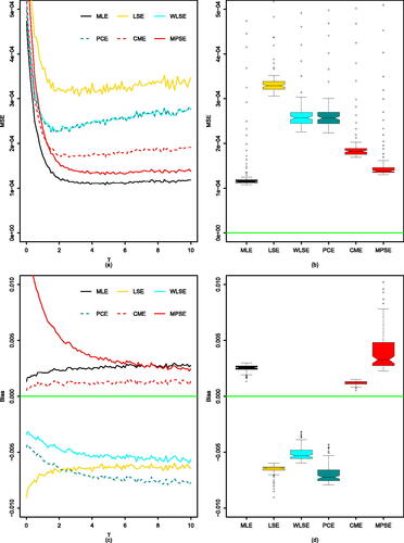
Fig. 2 (a) MSE of MLE, LSE, WLSE, PCE, CME, MPSE with respect to γ ($\epsilon =4,\varsigma =1$, and n = 20). (b) their corresponding Bias. (c) Boxplot of MSE values. (d) Boxplot of Bias values.

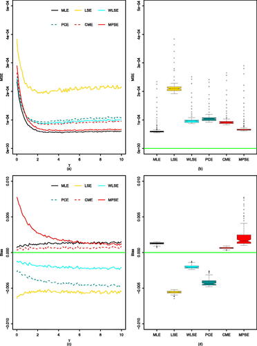
Table 1 True values of ${\mathcal{C}}_{\mathit{pmc}}^{\prime }$ and ${\mathcal{C}}_{\mathit{pmc}}$ along with average estimates based on MLE, LSE, WLSE, PCE, CME, MPSE along with their MSEs [$\gamma =0.01,5.0,10.0$].

PCI			MLE		LSE		WLSE		PCE		CME		MPSE
Parameters	γ	n	MLE	MSE	LSE	MSE	WLSE	MSE	PCE	MSE	CME	MSE	MPSE	MSE
${\mathcal{C}}_{\mathit{pmc}}$=0.4613
${\mathcal{C}}_{\mathit{pmc}}^{\prime }$=	0.01	10	0.46335	0.00047	0.45298	0.00069	0.45859	0.00052	0.45747	0.00049	0.46254	0.00054	0.47589	0.00065
0.4620	0.01	20	0.46269	0.00023	0.45555	0.00038	0.46072	0.00025	0.45934	0.00024	0.46234	0.00027	0.46978	0.00029
ε = 4.0	0.01	50	0.46231	0.00009	0.45762	0.00018	0.46167	0.00010	0.46070	0.00009	0.46218	0.00011	0.46554	0.00011
Ϛ=1.0	0.01	100	0.46218	0.00005	0.45856	0.00011	0.46189	0.00005	0.46126	0.00005	0.46209	0.00005	0.46394	0.00005
${\mathcal{C}}_{\mathit{pmc}}^{\prime }$=	5.0	10	0.55749	0.00011	0.54865	0.00031	0.54959	0.00025	0.54758	0.00025	0.55622	0.00018	0.55807	0.00013
0.55489	5.0	20	0.55635	0.00006	0.54943	0.00020	0.55299	0.00009	0.55066	0.00009	0.55571	0.00009	0.55665	0.00006
ε = 4.0	5.0	50	0.55539	0.00002	0.55036	0.00013	0.55431	0.00003	0.55263	0.00003	0.55515	0.00004	0.55552	0.00002
Ϛ=1.0	5.0	100	0.55515	0.00001	0.55124	0.00008	0.55467	0.00002	0.55356	0.00002	0.55502	0.00002	0.55521	0.00001
${\mathcal{C}}_{\mathit{pmc}}^{\prime }$=	10.0	10	0.56818	0.00011	0.55896	0.00035	0.55976	0.00028	0.55769	0.00028	0.56682	0.00019	0.56787	0.00014
0.56541	10.0	20	0.56691	0.00006	0.55991	0.00022	0.56332	0.00010	0.56087	0.00011	0.56625	0.00009	0.56664	0.00007
ε = 4.0	10.0	50	0.56598	0.00002	0.56086	0.00013	0.56480	0.00003	0.56305	0.00003	0.56568	0.00004	0.56586	0.00003
Ϛ=1.0	10.0	100	0.56573	0.00001	0.56168	0.00009	0.56520	0.00002	0.56404	0.00002	0.56556	0.00002	0.56565	0.00001
${\mathcal{C}}_{\mathit{pmc}}$=0.5263
${\mathcal{C}}_{\mathit{pmc}}^{\prime }$=	0.01	10	0.52751	0.00042	0.51549	0.00078	0.52055	0.00053	0.51896	0.00052	0.52625	0.00050	0.53768	0.00049
0.52655	0.01	20	0.52703	0.00021	0.51850	0.00044	0.52410	0.00024	0.52211	0.00024	0.52646	0.00025	0.53290	0.00023
ε = 5.0	0.01	50	0.52677	0.00009	0.52104	0.00022	0.52582	0.00009	0.52441	0.00009	0.52654	0.00010	0.52949	0.00009
Ϛ=1.0	0.01	100	0.52667	0.00004	0.52218	0.00014	0.52625	0.00005	0.52531	0.00005	0.52654	0.00005	0.52817	0.00004
${\mathcal{C}}_{\mathit{pmc}}^{\prime }$=	5.0	10	0.56718	0.00012	0.55789	0.00035	0.55887	0.00028	0.55676	0.00028	0.56585	0.00019	0.56778	0.00015
0.56443	5.0	20	0.56597	0.00006	0.55871	0.00022	0.56244	0.00010	0.55999	0.00011	0.56530	0.00009	0.56628	0.00007
ε = 5.0	5.0	50	0.56496	0.00003	0.55968	0.00014	0.56382	0.00003	0.56205	0.00004	0.56470	0.00004	0.56509	0.00003
Ϛ=1.0	5.0	100	0.56471	0.00001	0.56059	0.00009	0.56419	0.00002	0.56303	0.00001	0.56457	0.00002	0.56478	0.00001
${\mathcal{C}}_{\mathit{pmc}}^{\prime }$=	10.0	10	0.57324	0.00012	0.56379	0.00037	0.56461	0.00029	0.56248	0.00029	0.57185	0.00020	0.57293	0.00014
0.57039	10.0	20	0.57194	0.00006	0.56476	0.00022	0.56825	0.00011	0.56574	0.00011	0.57126	0.00010	0.57166	0.00007
ε = 5.0	10.0	50	0.57098	0.00002	0.56573	0.00013	0.56977	0.00003	0.56798	0.00004	0.57068	0.00004	0.57086	0.00003
Ϛ=1.0	10.0	100	0.57072	0.00001	0.56657	0.00009	0.57018	0.00002	0.56899	0.00002	0.57055	0.00002	0.57065	0.00001
${\mathcal{C}}_{\mathit{pmc}}$=0.5711
${\mathcal{C}}_{\mathit{pmc}}^{\prime }$=	0.01	10	0.57145	0.00019	0.56014	0.00057	0.56263	0.00039	0.56069	0.00040	0.56976	0.00028	0.57406	0.00018
0.57116	0.01	20	0.57129	0.00009	0.56290	0.00034	0.56754	0.00015	0.56507	0.00016	0.57050	0.00014	0.57296	0.00009
ε = 6.0	0.01	50	0.57126	0.00004	0.56543	0.00018	0.57002	0.00005	0.56825	0.00005	0.57092	0.00006	0.57209	0.00004
Ϛ=1.0	0.01	100	0.57121	0.00002	0.56655	0.00012	0.57067	0.00002	0.56948	0.00002	0.57104	0.00003	0.57169	0.00002
${\mathcal{C}}_{\mathit{pmc}}^{\prime }$=	5.0	10	0.57680	0.00013	0.56719	0.00038	0.56805	0.00031	0.56586	0.00031	0.57533	0.00021	0.57639	0.00016
0.57431	5.0	20	0.57579	0.00007	0.56821	0.00024	0.57206	0.00011	0.56949	0.00011	0.57506	0.00011	0.57587	0.00008
ε = 6.0	5.0	50	0.57474	0.00003	0.56929	0.00015	0.57349	0.00004	0.57167	0.00004	0.57442	0.00004	0.57482	0.00003
Ϛ=1.0	5.0	100	0.57459	0.00001	0.57028	0.00010	0.57405	0.00002	0.57282	0.00002	0.57444	0.00002	0.57463	0.00002
${\mathcal{C}}_{\mathit{pmc}}^{\prime }$=	10.0	10	0.57813	0.00014	0.56855	0.00039	0.56926	0.00032	0.56711	0.00032	0.57662	0.00024	0.57638	0.00032
0.57551	10.0	20	0.57706	0.00007	0.56972	0.00024	0.57328	0.00011	0.57070	0.00012	0.57636	0.00011	0.57669	0.00007
η = 6.0	10.0	50	0.57612	0.00003	0.57067	0.00014	0.57489	0.00004	0.57304	0.00004	0.57585	0.00004	0.57599	0.00003
ζ = 1.0	10.0	100	0.57584	0.00001	0.57158	0.00009	0.57529	0.00002	0.57407	0.00002	0.57567	0.00002	0.57577	0.00001

Further, the AW and CPs of BCIs based on $\mathcal{S}\mathcal{B},\mathcal{P}\mathcal{B},\mathcal{S}\mathcal{T}\mathcal{B},\mathcal{B}\mathcal{C}\mathcal{P}\mathcal{B}$ and $\mathcal{B}\mathcal{C}\mathcal{A}\mathcal{B}$ using considered methods of estimation for ${\mathcal{C}}_{\mathit{pmc}}^{\prime }$ are reported in Tables 2–7, respectively. The simulation results show that $\mathcal{B}\mathcal{C}\mathcal{A}$-boot provides smaller AW than their counterparts for almost all sample sizes and the considered methods of estimation and the order of performance of BCI is $\mathcal{B}\mathcal{C}\mathcal{A}\mathcal{B}<\mathcal{B}\mathcal{C}\mathcal{P}\mathcal{B}<\mathcal{S}TB<\mathcal{P}B<\mathcal{S}B$. In addition, we observe that $\mathcal{P}B$ CIs provide higher CP than their counterparts for all the considered methods of estimation and for almost all sample sizes.

Table 2 AW and CPs of BCIs of ${\mathcal{C}}_{\mathit{pmc}}^{\prime }$ using MLEs of the parameters [$\gamma =0.01,5.0,10.0$] along with true values of ${\mathcal{C}}_{\mathit{pmc}}^{\prime }$.

PCI			$\mathcal{S}$-boot		$\mathcal{P}$-boot		$\mathcal{T}$-boot		$\mathcal{B}\mathcal{C}\mathcal{P}$-boot		$\mathcal{B}\mathcal{C}\mathcal{A}$-boot
Parameter	γ	n	AW	CP	AW	CP	AW	CP	AW	CP	AW	CP
${\mathcal{C}}_{\mathit{pmc}}$=0.4613
${\mathcal{C}}_{\mathit{pmc}}^{\prime }$=	0.01	10	0.13227	0.887	0.11325	0.891	0.10578	0.885	0.08779	0.883	0.08312	0.879
0.4620	0.01	20	0.11768	0.903	0.097536	0.906	0.08779	0.901	0.06221	0.896	0.05985	0.893
ε = 4.0	0.01	50	0.09337	0.913	0.07456	0.915	0.06777	0.911	0.05373	0.909	0.05087	0.906
Ϛ=1.0	0.01	100	0.05887	0.927	0.04114	0.930	0.03775	0.924	0.03086	0.922	0.03042	0.920
${\mathcal{C}}_{\mathit{pmc}}^{\prime }$=	5.0	10	0.17236	0.888	0.15763	0.890	0.14622	0.886	0.12768	0.883	0.12114	0.881
0.5548	5.0	20	0.14554	0.904	0.12334	0.906	0.11327	0.902	0.10078	0.899	0.09674	0.886
ε = 4.0	5.0	50	0.12221	0.912	0.10458	0.914	0.09776	0.910	0.07683	0.907	0.07114	0.904
Ϛ=1.0	5.0	100	0.09887	0.926	0.07558	0.929	0.06677	0.923	0.04487	0.921	0.04056	0.918
${\mathcal{C}}_{\mathit{pmc}}^{\prime }$=	10.0	10	0.18587	0.889	0.16327	0.891	0.15437	0.886	0.13384	0.884	0.13077	0.882
0.5755	10.0	20	0.15563	0.903	0.13228	0.906	0.12236	0.901	0.10473	0.896	0.10087	0.893
ε = 4.0	10.0	50	0.12554	0.913	0.10767	0.916	0.09784	0.911	0.07578	0.909	0.07111	0.905
Ϛ=1.0	10.0	100	0.09986	0.928	0.07898	0.931	0.06453	0.926	0.04787	0.923	0.04221	0.921
${\mathcal{C}}_{\mathit{pmc}}$=0.5263
${\mathcal{C}}_{\mathit{pmc}}^{\prime }$=	0.01	10	0.15487	0.888	0.13783	0.892	0.12554	0.885	0.10587	0.884	0.10112	0.882
0.5265	0.01	20	0.12878	0.905	0.10348	0.907	0.09476	0.903	0.07226	0.902	0.07101	0.897
ε = 5.0	0.01	50	0.09997	0.914	0.07778	0.917	0.06869	0.911	0.05231	0.909	0.05089	0.906
Ϛ=1.0	0.01	100	0.07778	0.929	0.05676	0.933	0.04551	0.926	0.03886	0.924	0.03566	0.922
${\mathcal{C}}_{\mathit{pmc}}^{\prime }$=	5.0	10	0.17889	0.889	0.15767	0.892	0.14943	0.886	0.12476	0.883	0.12121	0.882
0.5644	5.0	20	0.14768	0.904	0.12889	0.906	0.11459	0.903	0.09986	0.901	0.09631	0.896
ε = 5.0	5.0	50	0.11656	0.912	0.09668	0.914	0.08778	0.910	0.06889	0.907	0.06236	0.904
Ϛ=1.0	5.0	100	0.08779	0.928	0.06582	0.932	0.05697	0.926	0.04211	0.923	0.04089	0.921
${\mathcal{C}}_{\mathit{pmc}}^{\prime }$=	10.0	10	0.18326	0.888	0.16395	0.891	0.15375	0.885	0.13787	0.884	0.13224	0.882
0.5703	10.0	20	0.15378	0.902	0.13672	0.905	0.12443	0.899	0.10787	0.896	0.10211	0.895
ε = 5.0	10.0	30	0.12882	0.912	0.10776	0.914	0.09669	0.909	0.07885	0.907	0.07336	0.905
Ϛ=1.0	10.0	100	0.09778	0.927	0.07556	0.929	0.06889	0.924	0.04675	0.924	0.04114	0.922
${\mathcal{C}}_{\mathit{pmc}}$=0.5711
${\mathcal{C}}_{\mathit{pmc}}^{\prime }$=	0.01	10	0.18786	0.889	0.16879	0.893	0.15668	0.886	0.14694	0.884	0.14221	0.881
0.5711	0.01	20	0.15487	0.904	0.13835	0.906	0.12774	0.901	0.10889	0.897	0.10332	0.894
η = 6.0	0.01	50	0.13116	0.914	0.11564	0.916	0.10476	0.912	0.08779	0.909	0.08326	0.907
Ϛ=1.0	0.01	100	0.10775	0.928	0.08679	0.931	0.07668	0.924	0.05884	0.923	0.05112	0.920
${\mathcal{C}}_{\mathit{pmc}}^{\prime }$=	5.0	10	0.19344	0.892	0.17482	0.894	0.16775	0.890	0.14677	0.887	0.14224	0.884
0.5743	5.0	20	0.16375	0.905	0.14396	0.906	0.13228	0.902	0.11774	0.899	0.11137	0.896
ε = 6.0	5.0	50	0.14111	0.915	0.12089	0.917	0.11768	0.913	0.09779	0.910	0.09312	0.907
Ϛ=1.0	5.0	100	0.10889	0.929	0.08774	0.932	0.07694	0.926	0.05898	0.923	0.05413	0.921
${\mathcal{C}}_{\mathit{pmc}}^{\prime }$=	10.0	10	0.19779	0.891	0.17595	0.894	0.16884	0.888	0.14562	0.885	0.14115	0.882
0.5755	10.0	20	0.16742	0.904	0.14774	0.907	0.13806	0.901	0.11779	0.897	0.11098	0.894
ε = 6.0	10.0	50	0.13657	0.914	0.11677	0.916	0.10793	0.912	0.08779	0.910	0.08237	0.908
Ϛ=1.0	10.0	100	0.10798	0.929	0.08335	0.932	0.07699	0.926	0.05556	0.924	0.05046	0.921

Table 3 AW and CPs of BCIs of ${\mathcal{C}}_{\mathit{pmc}}^{\prime }$ using LSEs of the parameters [$\gamma =0.01,5.0,10.0$] along with true values of ${\mathcal{C}}_{\mathit{pmc}}^{\prime }$ .

PCI			$\mathcal{S}$-boot		$\mathcal{P}$-boot		$\mathcal{T}$-boot		$\mathcal{B}\mathcal{C}\mathcal{P}$-boot		$\mathcal{B}\mathcal{C}\mathcal{A}$-boot
Parameter	γ	n	AW	CP	AW	CP	AW	CP	AW	CP	AW	CP
${\mathcal{C}}_{\mathit{pmc}}$=0.4613
${\mathcal{C}}_{\mathit{pmc}}^{\prime }$=	0.01	10	0.13221	0.884	0.11321	0.887	0.10575	0.884	0.08779	0.883	0.08312	0.879
0.4620	0.01	20	0.11762	0.901	0.09752	0.904	0.08777	0.902	0.06218	0.896	0.05981	0.894
ε = 4.0	0.01	50	0.09332	0.912	0.07452	0.912	0.06776	0.910	0.05374	0.907	0.05083	0.903
Ϛ=1.0	0.01	100	0.05884	0.924	0.04113	0.927	0.03774	0.923	0.03084	0.922	0.03040	0.920
${\mathcal{C}}_{\mathit{pmc}}^{\prime }$=	5.0	10	0.17233	0.882	0.15763	0.886	0.14622	0.884	0.12763	0.882	0.12112	0.879
0.5548	5.0	20	0.14552	0.904	0.12332	0.904	0.11326	0.902	0.10077	0.897	0.09672	0.884
ε = 4.0	5.0	50	0.12221	0.911	0.10456	0.912	0.09772	0.910	0.07681	0.904	0.07112	0.903
Ϛ=1.0	5.0	100	0.09885	0.925	0.07553	0.928	0.06675	0.923	0.04486	0.921	0.04057	0.919
${\mathcal{C}}_{\mathit{pmc}}^{\prime }$=	10.0	10	0.18584	0.884	0.16325	0.890	0.15433	0.884	0.13383	0.884	0.13074	0.882
0.5755	10.0	20	0.15564	0.903	0.13225	0.904	0.12236	0.901	0.10474	0.895	0.10089	0.893
ε = 4.0	10.0	50	0.12553	0.911	0.10766	0.914	0.09784	0.912	0.07575	0.907	0.07111	0.904
Ϛ=1.0	10.0	100	0.09985	0.929	0.07897	0.931	0.06457	0.926	0.04785	0.923	0.04223	0.921
${\mathcal{C}}_{\mathit{pmc}}$=0.5263
${\mathcal{C}}_{\mathit{pmc}}^{\prime }$=	0.01	10	0.15486	0.885	0.13784	0.890	0.12554	0.884	0.10587	0.882	0.10115	0.880
0.5264	0.01	20	0.12878	0.904	0.10348	0.906	0.09474	0.903	0.07224	0.902	0.07105	0.893
ε = 5.0	0.01	50	0.09995	0.914	0.07778	0.915	0.06867	0.911	0.05233	0.906	0.05086	0.903
Ϛ=1.0	0.01	100	0.07778	0.927	0.05677	0.930	0.04554	0.923	0.03889	0.922	0.03569	0.920
${\mathcal{C}}_{\mathit{pmc}}^{\prime }$=	5.0	10	0.17889	0.886	0.15766	0.890	0.14942	0.884	0.12476	0.883	0.12119	0.880
0.5644	5.0	20	0.14766	0.904	0.12887	0.906	0.11457	0.903	0.09985	0.902	0.09635	0.897
ε = 5.0	5.0	50	0.11656	0.909	0.09668	0.913	0.08777	0.908	0.06883	0.905	0.06237	0.901
Ϛ=1.0	5.0	100	0.08777	0.925	0.06582	0.928	0.05696	0.924	0.04210	0.923	0.04087	0.921
${\mathcal{C}}_{\mathit{pmc}}^{\prime }$=	10.0	10	0.18323	0.886	0.16392	0.889	0.15372	0.884	0.13785	0.883	0.13222	0.880
0.5703	10.0	20	0.15377	0.901	0.13674	0.904	0.12445	0.897	0.10788	0.894	0.10213	0.892
ε = 5.0	10.0	30	0.12883	0.913	0.10776	0.916	0.09669	0.910	0.07886	0.905	0.07335	0.903
Ϛ=1.0	10.0	100	0.09777	0.928	0.07557	0.931	0.06888	0.925	0.04677	0.923	0.04114	0.921
${\mathcal{C}}_{\mathit{pmc}}$=0.5711
${\mathcal{C}}_{\mathit{pmc}}^{\prime }$=	0.01	10	0.18783	0.886	0.16878	0.890	0.15666	0.884	0.14693	0.882	0.14223	0.880
0.5711	0.01	20	0.15485	0.904	0.13838	0.907	0.12774	0.902	0.10889	0.896	0.10334	0.892
ε = 6.0	0.01	50	0.13115	0.912	0.11565	0.914	0.10477	0.910	0.08776	0.907	0.08325	0.905
Ϛ=1.0	0.01	100	0.10774	0.925	0.08677	0.931	0.07665	0.924	0.05882	0.921	0.05113	0.920
${\mathcal{C}}_{\mathit{pmc}}^{\prime }$=	5.0	10	0.19343	0.891	0.17484	0.894	0.16777	0.892	0.14677	0.885	0.14226	0.882
0.5743	5.0	20	0.16376	0.904	0.14397	0.907	0.13226	0.903	0.11772	0.898	0.11137	0.894
ε = 6.0	5.0	50	0.14114	0.915	0.12087	0.917	0.11767	0.913	0.09782	0.908	0.09311	0.906
Ϛ=1.0	5.0	100	0.10887	0.927	0.08773	0.930	0.07692	0.927	0.05896	0.924	0.05413	0.921
${\mathcal{C}}_{\mathit{pmc}}^{\prime }$=	10.0	10	0.19777	0.890	0.17594	0.892	0.16883	0.884	0.14563	0.884	0.14114	0.881
0.5755	10.0	20	0.16741	0.903	0.14774	0.906	0.13806	0.901	0.11782	0.897	0.11095	0.892
ε = 6.0	10.0	50	0.13657	0.914	0.11681	0.917	0.10798	0.912	0.08780	0.909	0.08239	0.905
Ϛ=1.0	10.0	100	0.10798	0.928	0.08337	0.931	0.07699	0.925	0.05557	0.923	0.05047	0.921

Table 4 AW and CPs of BCIs of ${\mathcal{C}}_{\mathit{pmc}}^{\prime }$ using WLSEs of the parameters [$\gamma =0.01,5.0,10.0$] along with true values of ${\mathcal{C}}_{\mathit{pmc}}^{\prime }$.

PCI			$\mathcal{S}$-boot		$\mathcal{P}$-boot		$\mathcal{T}$-boot		$\mathcal{B}\mathcal{C}\mathcal{P}$-boot		$\mathcal{B}\mathcal{C}\mathcal{A}$-boot
Parameter	γ	n	AW	CP	AW	CP	AW	CP	AW	CP	AW	CP
${\mathcal{C}}_{\mathit{pmc}}$=0.4613
${\mathcal{C}}_{\mathit{pmc}}^{\prime }$=	0.01	10	0.13222	0.885	0.11320	0.890	0.10573	0.882	0.08777	0.883	0.08310	0.877
0.4620	0.01	20	0.11763	0.902	0.09750	0.904	0.08774	0.901	0.06217	0.894	0.05982	0.892
ε = 4.0	0.01	50	0.09334	0.913	0.07453	0.914	0.06774	0.910	0.05371	0.908	0.05084	0.904
Ϛ=1.0	0.01	100	0.05883	0.924	0.04111	0.928	0.03774	0.923	0.03084	0.922	0.03040	0.920
${\mathcal{C}}_{\mathit{pmc}}^{\prime }$=	5.0	10	0.17232	0.884	0.15761	0.888	0.14621	0.884	0.12764	0.882	0.12111	0.880
0.5548	5.0	20	0.14551	0.903	0.12331	0.904	0.11324	0.902	0.10076	0.896	0.09672	0.883
ε = 4.0	5.0	50	0.12220	0.910	0.10454	0.912	0.09771	0.910	0.07680	0.904	0.07111	0.902
Ϛ=1.0	5.0	100	0.09884	0.924	0.07554	0.929	0.06674	0.923	0.04485	0.921	0.04054	0.918
${\mathcal{C}}_{\mathit{pmc}}^{\prime }$=	10.0	10	0.18585	0.886	0.16324	0.890	0.15433	0.884	0.13383	0.884	0.13074	0.882
0.5755	10.0	20	0.15563	0.903	0.13224	0.904	0.12234	0.902	0.10472	0.894	0.10087	0.891
ε = 4.0	10.0	50	0.12551	0.912	0.10764	0.914	0.09782	0.911	0.07574	0.908	0.07111	0.904
Ϛ=1.0	10.0	100	0.09984	0.928	0.07895	0.931	0.06455	0.926	0.04784	0.922	0.04220	0.921
${\mathcal{C}}_{\mathit{pmc}}$=0.5263
${\mathcal{C}}_{\mathit{pmc}}^{\prime }$=	0.01	10	0.15484	0.886	0.13781	0.891	0.12551	0.884	0.10584	0.881	0.10112	0.880
0.5264	0.01	20	0.12876	0.903	0.10346	0.906	0.09473	0.903	0.07223	0.902	0.07101	0.894
ε = 5.0	0.01	50	0.09994	0.913	0.07776	0.914	0.06865	0.911	0.05231	0.907	0.05086	0.903
Ϛ=1.0	0.01	100	0.07777	0.927	0.05674	0.931	0.04551	0.924	0.03886	0.923	0.03566	0.921
${\mathcal{C}}_{\mathit{pmc}}^{\prime }$=	5.0	10	0.17886	0.887	0.15764	0.891	0.14940	0.884	0.12473	0.883	0.12118	0.880
0.5644	5.0	20	0.14764	0.903	0.12886	0.905	0.11456	0.903	0.09984	0.901	0.09630	0.894
ε = 5.0	5.0	50	0.11653	0.910	0.09666	0.913	0.08774	0.910	0.06883	0.906	0.06235	0.902
Ϛ=1.0	5.0	100	0.08776	0.926	0.06581	0.930	0.05694	0.925	0.04210	0.923	0.04086	0.920
${\mathcal{C}}_{\mathit{pmc}}^{\prime }$=	10.0	10	0.18323	0.886	0.16392	0.889	0.15372	0.884	0.13785	0.883	0.13222	0.880
0.5703	10.0	20	0.15376	0.901	0.13671	0.903	0.12441	0.896	0.10785	0.894	0.10210	0.893
ε = 5.0	10.0	30	0.12881	0.912	0.10774	0.914	0.09668	0.910	0.07884	0.906	0.07334	0.904
Ϛ=1.0	10.0	100	0.09776	0.928	0.07555	0.930	0.06886	0.924	0.04674	0.924	0.04112	0.921
${\mathcal{C}}_{\mathit{pmc}}$=0.5711
${\mathcal{C}}_{\mathit{pmc}}^{\prime }$=	0.01	10	0.18782	0.887	0.16876	0.891	0.15664	0.884	0.14691	0.881	0.14221	0.880
0.5711	0.01	20	0.15484	0.903	0.13835	0.904	0.12771	0.901	0.10886	0.894	0.10331	0.892
ε = 6.0	0.01	50	0.13114	0.912	0.11562	0.914	0.10474	0.912	0.08776	0.907	0.08324	0.905
Ϛ=1.0	0.01	100	0.10773	0.926	0.08676	0.931	0.07664	0.924	0.05881	0.921	0.05111	0.920
${\mathcal{C}}_{\mathit{pmc}}^{\prime }$=	5.0	10	0.19342	0.891	0.17482	0.893	0.16775	0.891	0.14676	0.884	0.14224	0.882
0.5743	5.0	20	0.16373	0.904	0.14396	0.907	0.13225	0.903	0.11771	0.898	0.11137	0.894
ε = 6.0	5.0	50	0.14112	0.914	0.12086	0.917	0.11765	0.912	0.09781	0.908	0.09310	0.906
Ϛ=1.0	5.0	100	0.10886	0.928	0.08772	0.930	0.07691	0.927	0.05896	0.924	0.05412	0.921
${\mathcal{C}}_{\mathit{pmc}}^{\prime }$=	10.0	10	0.19776	0.890	0.17593	0.893	0.16882	0.884	0.14561	0.884	0.14112	0.880
0.5755	10.0	20	0.16740	0.903	0.14772	0.905	0.13806	0.901	0.11779	0.897	0.11096	0.893
ε = 6.0	10.0	50	0.13656	0.915	0.11679	0.917	0.10795	0.912	0.08779	0.908	0.08236	0.906
Ϛ=1.0	10.0	100	0.10796	0.929	0.08335	0.931	0.07697	0.926	0.05556	0.923	0.05046	0.920

Table 5 AW and CPs of BCIs of ${\mathcal{C}}_{\mathit{pmc}}^{\prime }$ using PCEs of the parameters [$\gamma =0.01,5.0,10.0$] along with true values of ${\mathcal{C}}_{\mathit{pmc}}^{\prime }$.

PCI			$\mathcal{S}$-boot		$\mathcal{P}$-boot		$\mathcal{T}$-boot		$\mathcal{B}\mathcal{C}\mathcal{P}$-boot		$\mathcal{B}\mathcal{C}\mathcal{A}$-boot
Parameter	γ	n	AW	CP	AW	CP	AW	CP	AW	CP	AW	CP
${\mathcal{C}}_{\mathit{pmc}}$=0.4613
${\mathcal{C}}_{\mathit{pmc}}^{\prime }$=	0.01	10	0.13229	0.886	0.11327	0.891	0.10579	0.885	0.08778	0.883	0.08315	0.878
0.4620	0.01	20	0.11769	0.904	0.09754	0.906	0.08781	0.902	0.06224	0.895	0.05987	0.893
ε = 4.0	0.01	50	0.09338	0.912	0.07458	0.915	0.06779	0.910	0.05375	0.909	0.05088	0.906
Ϛ=1.0	0.01	100	0.05888	0.927	0.04115	0.930	0.03777	0.924	0.03087	0.922	0.03044	0.920
${\mathcal{C}}_{\mathit{pmc}}^{\prime }$=	5.0	10	0.17238	0.888	0.15765	0.890	0.14624	0.886	0.12769	0.884	0.12116	0.881
0.5548	5.0	20	0.14556	0.904	0.12337	0.906	0.11329	0.901	0.10078	0.898	0.09677	0.885
ε = 4.0	5.0	50	0.12224	0.913	0.10459	0.915	0.09779	0.911	0.07686	0.906	0.07117	0.904
Ϛ=1.0	5.0	100	0.09889	0.925	0.07559	0.928	0.06679	0.923	0.04488	0.921	0.04057	0.919
${\mathcal{C}}_{\mathit{pmc}}^{\prime }$=	10.0	10	0.18588	0.889	0.16329	0.891	0.15438	0.886	0.13386	0.884	0.13079	0.884
0.5755	10.0	20	0.15564	0.903	0.13229	0.906	0.12237	0.901	0.10475	0.896	0.10088	0.893
ε = 4.0	10.0	50	0.12555	0.913	0.10769	0.915	0.09786	0.911	0.07579	0.908	0.07114	0.905
Ϛ=1.0	10.0	100	0.09988	0.928	0.07899	0.930	0.06455	0.926	0.04788	0.924	0.04225	0.922
${\mathcal{C}}_{\mathit{pmc}}$=0.5263
${\mathcal{C}}_{\mathit{pmc}}^{\prime }$=	0.01	10	0.15488	0.888	0.13786	0.891	0.12557	0.885	0.10589	0.883	0.10114	0.881
0.5265	0.01	20	0.12879	0.905	0.10349	0.907	0.09477	0.903	0.07228	0.901	0.07105	0.896
ε = 5.0	0.01	50	0.09999	0.914	0.07782	0.916	0.06869	0.910	0.05234	0.908	0.05088	0.906
Ϛ=1.0	0.01	100	0.07779	0.928	0.05677	0.931	0.04554	0.926	0.03889	0.924	0.03569	0.922
${\mathcal{C}}_{\mathit{pmc}}^{\prime }$=	5.0	10	0.17892	0.889	0.15769	0.891	0.14946	0.886	0.12479	0.884	0.12125	0.882
0.5644	5.0	20	0.14769	0.904	0.12893	0.906	0.11463	0.903	0.09987	0.901	0.09636	0.897
ε = 5.0	5.0	50	0.11658	0.913	0.09673	0.915	0.08779	0.911	0.06893	0.906	0.06238	0.904
Ϛ=1.0	5.0	100	0.08778	0.927	0.06584	0.930	0.05696	0.925	0.04215	0.923	0.04088	0.921
${\mathcal{C}}_{\mathit{pmc}}^{\prime }$=	10.0	10	0.18328	0.889	0.16397	0.891	0.15377	0.886	0.13789	0.884	0.13223	0.882
0.5703	10.0	20	0.15377	0.902	0.13675	0.905	0.12447	0.898	0.10789	0.896	0.10214	0.894
ε = 5.0	10.0	30	0.12884	0.913	0.10777	0.915	0.09668	0.910	0.07888	0.907	0.07339	0.905
Ϛ=1.0	10.0	100	0.09779	0.927	0.07558	0.929	0.06888	0.925	0.04677	0.924	0.04116	0.922
${\mathcal{C}}_{\mathit{pmc}}$=0.5711
${\mathcal{C}}_{\mathit{pmc}}^{\prime }$=	0.01	10	0.18788	0.888	0.16879	0.892	0.15669	0.886	0.14696	0.884	0.14224	0.882
0.5711	0.01	20	0.15489	0.903	0.13838	0.906	0.12777	0.901	0.10888	0.896	0.10331	0.893
η = 6.0	0.01	50	0.13118	0.913	0.11567	0.916	0.10477	0.911	0.08779	0.909	0.08327	0.906
Ϛ=1.0	0.01	100	0.10777	0.927	0.08679	0.930	0.07669	0.924	0.05887	0.923	0.05114	0.921
${\mathcal{C}}_{\mathit{pmc}}^{\prime }$=	5.0	10	0.19346	0.891	0.17484	0.894	0.16777	0.889	0.14679	0.887	0.14226	0.885
0.5743	5.0	20	0.16377	0.905	0.14398	0.906	0.13229	0.903	0.11777	0.899	0.11136	0.897
ε = 6.0	5.0	50	0.14114	0.914	0.12089	0.916	0.11769	0.912	0.09779	0.910	0.09315	0.907
Ϛ=1.0	5.0	100	0.10888	0.929	0.08777	0.931	0.07694	0.926	0.05899	0.924	0.05415	0.922
${\mathcal{C}}_{\mathit{pmc}}^{\prime }$=	10.0	10	0.19779	0.892	0.17597	0.894	0.16887	0.889	0.14565	0.884	0.14118	0.882
0.5755	10.0	20	0.16744	0.905	0.14777	0.907	0.13809	0.902	0.11778	0.896	0.11096	0.894
ε = 6.0	10.0	50	0.13658	0.914	0.11676	0.916	0.10794	0.912	0.08778	0.910	0.08239	0.907
Ϛ=1.0	10.0	100	0.10799	0.929	0.08336	0.931	0.07698	0.926	0.05558	0.923	0.05049	0.921

Table 6 AW and CPs of BCIs of ${\mathcal{C}}_{\mathit{pmc}}^{\prime }$ using CMEs of the parameters [$\gamma =0.01,5.0,10.0$] along with true values of ${\mathcal{C}}_{\mathit{pmc}}^{\prime }$.

PCI			$\mathcal{S}$-boot		$\mathcal{P}$-boot		$\mathcal{T}$-boot		$\mathcal{B}\mathcal{C}\mathcal{P}$-boot		$\mathcal{B}\mathcal{C}\mathcal{A}$-boot
Parameter	γ	n	AW	CP	AW	CP	AW	CP	AW	CP	AW	CP
${\mathcal{C}}_{\mathit{pmc}}$=0.4613
${\mathcal{C}}_{\mathit{pmc}}^{\prime }$=	0.01	10	0.13224	0.883	0.11324	0.886	0.10577	0.884	0.08779	0.882	0.08315	0.879
0.4620	0.01	20	0.11766	0.902	0.09757	0.904	0.08779	0.901	0.06219	0.896	0.05986	0.893
ε = 4.0	0.01	50	0.09335	0.913	0.07458	0.915	0.06779	0.911	0.05377	0.908	0.05086	0.904
Ϛ=1.0	0.01	100	0.05886	0.923	0.04117	0.926	0.03778	0.922	0.03087	0.921	0.03044	0.918
${\mathcal{C}}_{\mathit{pmc}}^{\prime }$=	5.0	10	0.17235	0.884	0.15768	0.887	0.14627	0.883	0.12763	0.882	0.12115	0.879
0.5548	5.0	20	0.14555	0.904	0.12337	0.906	0.11327	0.902	0.10079	0.895	0.09674	0.889
ε = 4.0	5.0	50	0.12224	0.912	0.10459	0.914	0.09774	0.910	0.07684	0.907	0.07114	0.903
Ϛ=1.0	5.0	100	0.09888	0.925	0.07554	0.927	0.06677	0.923	0.04488	0.922	0.04058	0.919
${\mathcal{C}}_{\mathit{pmc}}^{\prime }$=	10.0	10	0.18586	0.885	0.16328	0.891	0.15436	0.885	0.13384	0.885	0.13077	0.884
0.5755	10.0	20	0.15567	0.903	0.13226	0.904	0.12238	0.901	0.10477	0.895	0.10088	0.892
ε = 4.0	10.0	50	0.12555	0.911	0.10768	0.914	0.09788	0.912	0.07577	0.906	0.07114	0.904
Ϛ=1.0	10.0	100	0.09988	0.929	0.07899	0.931	0.06459	0.926	0.04788	0.924	0.04226	0.921
${\mathcal{C}}_{\mathit{pmc}}$=0.5263
${\mathcal{C}}_{\mathit{pmc}}^{\prime }$=	0.01	10	0.15488	0.885	0.13787	0.890	0.12556	0.884	0.10589	0.883	0.10114	0.880
0.5264	0.01	20	0.12877	0.904	0.10349	0.906	0.09474	0.902	0.07227	0.902	0.07104	0.896
ε = 5.0	0.01	50	0.09994	0.913	0.07779	0.915	0.06869	0.911	0.05237	0.906	0.05089	0.903
Ϛ=1.0	0.01	100	0.07777	0.926	0.05679	0.930	0.04558	0.923	0.03888	0.922	0.03568	0.920
${\mathcal{C}}_{\mathit{pmc}}^{\prime }$=	5.0	10	0.17888	0.886	0.15768	0.890	0.14944	0.884	0.12477	0.884	0.12118	0.881
0.5644	5.0	20	0.14768	0.904	0.12886	0.906	0.11459	0.903	0.09988	0.902	0.09634	0.898
ε = 5.0	5.0	50	0.11656	0.910	0.09669	0.913	0.08778	0.908	0.06886	0.904	0.06239	0.901
Ϛ=1.0	5.0	100	0.08779	0.924	0.06586	0.928	0.05699	0.923	0.04212	0.922	0.04086	0.920
${\mathcal{C}}_{\mathit{pmc}}^{\prime }$=	10.0	10	0.18325	0.887	0.16396	0.889	0.15375	0.884	0.13787	0.884	0.13224	0.881
0.5703	10.0	20	0.15378	0.902	0.13677	0.905	0.12446	0.898	0.10789	0.894	0.10215	0.892
ε = 5.0	10.0	30	0.12884	0.913	0.10777	0.916	0.09668	0.910	0.07887	0.906	0.07338	0.903
Ϛ=1.0	10.0	100	0.09778	0.928	0.07558	0.930	0.06887	0.925	0.04678	0.923	0.04116	0.921
${\mathcal{C}}_{\mathit{pmc}}$=0.5711
${\mathcal{C}}_{\mathit{pmc}}^{\prime }$=	0.01	10	0.18787	0.888	0.16879	0.890	0.15668	0.884	0.14696	0.883	0.14226	0.881
0.5711	0.01	20	0.15488	0.904	0.13839	0.907	0.12775	0.902	0.10889	0.897	0.10334	0.894
ε = 6.0	0.01	50	0.13118	0.912	0.11566	0.914	0.10478	0.910	0.08777	0.907	0.08328	0.905
Ϛ=1.0	0.01	100	0.10775	0.925	0.08678	0.931	0.07667	0.924	0.05886	0.922	0.05114	0.920
${\mathcal{C}}_{pm}^{\prime }$=	5.0	10	0.19345	0.891	0.17486	0.894	0.16778	0.890	0.14677	0.887	0.14228	0.883
0.5743	5.0	20	0.16379	0.904	0.14398	0.907	0.13227	0.903	0.11774	0.899	0.11136	0.894
ε = 6.0	5.0	50	0.14115	0.915	0.12088	0.917	0.11769	0.913	0.09784	0.909	0.09315	0.905
Ϛ=1.0	5.0	100	0.10888	0.926	0.08777	0.929	0.07697	0.925	0.05897	0.923	0.05415	0.921
${\mathcal{C}}_{\mathit{pmc}}^{\prime }$=	10.0	10	0.19778	0.890	0.17595	0.892	0.16884	0.884	0.14566	0.885	0.14113	0.881
0.5755	10.0	20	0.16744	0.903	0.14776	0.906	0.13806	0.901	0.11784	0.898	0.11097	0.895
ε = 6.0	10.0	50	0.13659	0.913	0.11684	0.917	0.10799	0.912	0.08784	0.909	0.08244	0.906
Ϛ=1.0	10.0	100	0.10799	0.927	0.08342	0.931	0.07704	0.925	0.05563	0.924	0.05048	0.921

Table 7 AW and CPs of BCIs of ${\mathcal{C}}_{\mathit{pmc}}^{\prime }$ using MPSEs of the parameters [$\gamma =0.01,5.0,10.0$] along with true values of ${\mathcal{C}}_{\mathit{pmc}}^{\prime }$.

PCI			$\mathcal{S}$-boot		$\mathcal{P}$-boot		$\mathcal{T}$-boot		$\mathcal{B}\mathcal{C}\mathcal{P}$-boot		$\mathcal{B}\mathcal{C}\mathcal{A}$-boot
Parameter	γ	n	AW	CP	AW	CP	AW	CP	AW	CP	AW	CP
${\mathcal{C}}_{\mathit{pmc}}$=0.4613
${\mathcal{C}}_{\mathit{pmc}}^{\prime }$=	0.01	10	0.13224	0.886	0.11321	0.890	0.10574	0.884	0.08778	0.883	0.08311	0.878
0.4620	0.01	20	0.11764	0.902	0.09751	0.905	0.08776	0.901	0.06218	0.895	0.05983	0.892
ε = 4.0	0.01	50	0.09336	0.913	0.07454	0.915	0.06775	0.910	0.05372	0.908	0.05085	0.905
Ϛ=1.0	0.01	100	0.05884	0.926	0.04112	0.929	0.03775	0.923	0.03085	0.922	0.03041	0.920
${\mathcal{C}}_{\mathit{pmc}}^{\prime }$=	5.0	10	0.17233	0.886	0.15761	0.889	0.14621	0.885	0.12766	0.882	0.12112	0.880
0.5548	5.0	20	0.14552	0.903	0.12332	0.905	0.11324	0.902	0.10077	0.897	0.09672	0.884
ε = 4.0	5.0	50	0.12220	0.911	0.10454	0.913	0.09771	0.910	0.07681	0.905	0.07111	0.902
Ϛ=1.0	5.0	100	0.09886	0.926	0.07558	0.929	0.06674	0.923	0.04486	0.921	0.04055	0.917
${\mathcal{C}}_{\mathit{pmc}}^{\prime }$=	10.0	10	0.18586	0.888	0.16326	0.891	0.15435	0.884	0.13384	0.884	0.13075	0.881
0.5755	10.0	20	0.15562	0.903	0.13226	0.905	0.12234	0.901	0.10471	0.895	0.10087	0.892
ε = 4.0	10.0	50	0.12552	0.913	0.10766	0.916	0.09783	0.911	0.07576	0.908	0.07111	0.905
Ϛ=1.0	10.0	100	0.09985	0.928	0.07897	0.931	0.06454	0.926	0.04786	0.922	0.04221	0.921
${\mathcal{C}}_{\mathit{pmc}}$=0.5263
${\mathcal{C}}_{\mathit{pmc}}^{\prime }$=	0.01	10	0.15486	0.887	0.13782	0.891	0.12552	0.884	0.10586	0.882	0.10112	0.881
0.5264	0.01	20	0.12877	0.904	0.10347	0.906	0.09474	0.903	0.07224	0.902	0.07102	0.896
ε = 5.0	0.01	50	0.09996	0.914	0.07777	0.915	0.06867	0.911	0.05232	0.908	0.05088	0.905
Ϛ=1.0	0.01	100	0.07779	0.928	0.05675	0.933	0.04552	0.926	0.03887	0.924	0.03567	0.922
${\mathcal{C}}_{\mathit{pmc}}^{\prime }$=	5.0	10	0.17887	0.888	0.15766	0.892	0.14941	0.885	0.12475	0.883	0.12119	0.881
0.5644	5.0	20	0.14766	0.903	0.12887	0.906	0.11457	0.903	0.09985	0.901	0.09630	0.895
ε = 5.0	5.0	50	0.11654	0.911	0.09667	0.914	0.08776	0.910	0.06888	0.907	0.06235	0.903
Ϛ=1.0	5.0	100	0.08778	0.927	0.06581	0.930	0.05696	0.925	0.04210	0.923	0.04088	0.920
${\mathcal{C}}_{\mathit{pmc}}^{\prime }$=	10.0	10	0.18324	0.887	0.16393	0.890	0.15374	0.884	0.13786	0.884	0.13223	0.881
0.5703	10.0	20	0.15377	0.901	0.13672	0.904	0.12442	0.897	0.10786	0.895	0.10210	0.894
ε = 5.0	10.0	30	0.12881	0.913	0.10774	0.915	0.09669	0.910	0.07884	0.907	0.07335	0.905
Ϛ=1.0	10.0	100	0.09778	0.928	0.07556	0.930	0.06888	0.925	0.04675	0.924	0.04113	0.921
${\mathcal{C}}_{\mathit{pmc}}$=0.5711
${\mathcal{C}}_{\mathit{pmc}}^{\prime }$=	0.01	10	0.18784	0.888	0.16877	0.892	0.15666	0.885	0.14693	0.882	0.14221	0.881
0.5711	0.01	20	0.15486	0.903	0.13834	0.905	0.12773	0.901	0.10888	0.896	0.10332	0.893
ε = 6.0	0.01	50	0.13115	0.913	0.11563	0.915	0.10475	0.912	0.08778	0.908	0.08325	0.906
Ϛ=1.0	0.01	100	0.10774	0.927	0.08677	0.931	0.07666	0.924	0.05883	0.922	0.05111	0.921
${\mathcal{C}}_{pm}^{\prime }$=	5.0	10	0.19344	0.891	0.17483	0.893	0.16774	0.891	0.14676	0.886	0.14223	0.883
0.5743	5.0	20	0.16374	0.904	0.14397	0.906	0.13226	0.903	0.11772	0.898	0.11138	0.895
ε = 6.0	5.0	50	0.14112	0.915	0.12088	0.917	0.11767	0.914	0.09781	0.909	0.09311	0.907
Ϛ=1.0	5.0	100	0.10888	0.929	0.08772	0.931	0.07692	0.927	0.05897	0.924	0.05414	0.922
${\mathcal{C}}_{\mathit{pmc}}^{\prime }$=	10.0	10	0.19778	0.890	0.17594	0.893	0.16883	0.886	0.14562	0.884	0.14114	0.881
0.5755	10.0	20	0.16741	0.903	0.14772	0.906	0.13805	0.901	0.11778	0.896	0.11097	0.893
ε = 6.0	10.0	50	0.13658	0.914	0.11678	0.916	0.10795	0.913	0.08779	0.909	0.08237	0.907
Ϛ=1.0	10.0	100	0.10797	0.928	0.08334	0.931	0.07698	0.926	0.05556	0.924	0.05047	0.921

5 Applications in electronic industries data

In the last 50 years or so, we have witnessed how technology played a vital role in all spheres of knowledge and how technologies have eased our work by increasing productivity and generating quality products that cater to the needs of the customers. We are aware that the manufacturing industries are susceptible to failures in their manufacturing stages and at the end of the process the generated products may not meet the specifications. Due to this, both the manufacturer and customers may face losses. Motivated by the above, proposed methodology is applied to verify whether the product of a specific company meets the desired specifications and for this purpose, in this section, we re-analyze three real data sets which are taken from electronic industries to demonstrate the performance of the point estimates of ${\mathcal{C}}_{\mathit{pmc}}^{\prime }$ and ${\mathcal{C}}_{\mathit{pmc}}$ (see, Saha, Dey, and Wang 2022) using considered methods of estimation. Further, the width of BCIs ($\mathcal{S}\mathcal{B}$, $\mathcal{P}\mathcal{B},\mathcal{S}\mathcal{T}\mathcal{B},\mathcal{B}\mathcal{C}\mathcal{P}\mathcal{B}$ and $\mathcal{B}\mathcal{C}\mathcal{A}\mathcal{B}$) using considered methods of estimation for the PCIs ${\mathcal{C}}_{\mathit{pmc}}^{\prime }$ and ${\mathcal{C}}_{\mathit{pmc}}$ are obtained and reported in Tables 8–9, respectively.

Table 8 Estimates of ${\mathcal{C}}_{\mathit{pmc}}^{\prime }$ and ${\mathcal{C}}_{\mathit{pmc}}$ along with width of BCIs based on data set I [$\gamma =0.01, c_0=10, c_1=20, c_2=15, t=10$].

Methods of	Classical	Width of BCIs
estimation	estimates	$\mathcal{S}$-boot	$\mathcal{P}$-boot	$\mathcal{T}$-boot	$\mathcal{B}\mathcal{C}\mathcal{P}$-boot	$\mathcal{B}\mathcal{C}\mathcal{A}$-boot
MLE	${\mathcal{C}}_{\mathit{pmc}}^{\mathit{mle}}$=1.65908	0.16187	0.14224	0.13544	0.13224	0.12723
	${\mathcal{C}}_{\mathit{pmc}}^{\prime \mathit{mle}}$=1.39628	0.14309	0.12684	0.12457	0.11866	0.10903
LSE	${\mathcal{C}}_{\mathit{pmc}}^{\mathit{lse}}$=1.65989	0.16673	0.14677	0.13778	0.13765	0.12834
	${\mathcal{C}}_{\mathit{pmc}}^{\prime \mathit{lse}}$=1.39889	0.14784	0.12986	0.12887	0.12107	0.11012
WLSE	${\mathcal{C}}_{\mathit{pmc}}^{\mathit{wlse}}$=1.65914	0.16204	0.14237	0.13578	0.13375	0.12748
	${\mathcal{C}}_{\mathit{pmc}}^{\prime \mathit{wlse}}$=1.39636	0.14314	0.12784	0.12611	0.11876	0.10944
PCE	${\mathcal{C}}_{\mathit{pmc}}^{\mathit{pce}}$=1.65987	0.16415	0.14546	0.13778	0.13659	0.12887
	${\mathcal{C}}_{\mathit{pmc}}^{\prime \mathit{pce}}$=1.39844	0.14413	0.12879	0.12784	0.11912	0.11034
CME	${\mathcal{C}}_{\mathit{pmc}}^{\mathit{cme}}$=1.66211	0.16673	0.14783	0.13889	0.13702	0.12988
	${\mathcal{C}}_{\mathit{pmc}}^{\prime \mathit{mle}}$=1.40114	0.14879	0.13111	0.13099	0.12116	0.11324
MPSE	${\mathcal{C}}_{\mathit{pmc}}^{\mathit{mpse}}$=1.65788	0.16166	0.14176	0.13438	0.13203	0.12679
	${\mathcal{C}}_{\mathit{pmc}}^{\prime \mathit{mpse}}$=1.33655	0.14277	0.12437	0.12377	0.11748	0.10878

Table 9 Estimates of ${\mathcal{C}}_{\mathit{pmc}}^{\prime }$ and ${\mathcal{C}}_{\mathit{pmc}}$ along with width of BCIs based on data set II [$\gamma =5.0, c_0=10, c_1=20, c_2=15, t=0.5$].

Methods of	Classical	Width of BCIs
estimation	estimates	$\mathcal{S}$-boot	$\mathcal{P}$-boot	$\mathcal{T}$-boot	$\mathcal{B}\mathcal{C}\mathcal{P}$-boot	$\mathcal{B}\mathcal{C}\mathcal{A}$-boot
MLE	${\mathcal{C}}_{\mathit{pmc}}^{\mathit{mle}}$=0.91565	0.19094	0.17812	0.15889	0.14778	0.14076
	${\mathcal{C}}_{\mathit{pmc}}^{\prime \mathit{mle}}$=0.91629	0.19198	0.17567	0.15476	0.14893	0.14121
LSE	${\mathcal{C}}_{\mathit{pmc}}^{\mathit{lse}}$=0.92261	0.19116	0.17838	0.16018	0.14794	0.14119
	${\widehat{\mathcal{C}}}_{\mathit{pmc}}^{\prime \mathit{lse}}$=0.92568	0.19217	0.17573	0.15509	0.14911	0.14137
WLSE	${\widehat{\mathcal{C}}}_{\mathit{pmc}}^{\mathit{wlse}}$=0.92221	0.19110	0.17833	0.16014	0.14789	0.14117
	${\widehat{\mathcal{C}}}_{\mathit{pmc}}^{\prime \mathit{wlse}}$=0.92574	0.19204	0.17569	0.15502	0.14907	0.14131
PCE	${\widehat{\mathcal{C}}}_{\mathit{pmc}}^{\mathit{pce}}$=0.92788	0.19111	0.17826	0.15898	0.14794	0.72487
	${\widehat{\mathcal{C}}}_{\mathit{pmc}}^{\prime \mathit{pce}}$=0.93112	0.19216	0.17586	0.15477	0.14903	0.14142
CME	${\widehat{\mathcal{C}}}_{\mathit{pmc}}^{\mathit{cme}}$=0.93147	0.19133	0.17846	0.15902	0.14805	0.72521
	${\widehat{\mathcal{C}}}_{\mathit{pmc}}^{\prime \mathit{mle}}$=0.93226	0.19278	0.17603	0.15506	0.14925	0.75189
MPSE	${\widehat{\mathcal{C}}}_{\mathit{pmc}}^{\mathit{mpse}}$=0.90658	0.19044	0.17798	0.15878	0.14772	0.72438
	${\widehat{\mathcal{C}}}_{\mathit{pmc}}^{\prime \mathit{mpse}}$=0.90779	0.19187	0.17563	0.15462	0.14885	0.14127

Data Set I: Thickness of the membrane of color STN display process.

This data set is taken from Chen and Chen (2004) and consists of the thickness of the membrane of color STN display. The specification limits were $12000\pm 500 A^0$ (where $1 A^0={10}^{-7} mm$), that is, the upper and the lower specification limits were set as $\mathcal{U}=12500,\mathcal{L}=11500$ and the target value was set to $\mathcal{T}=12000$. If the thickness of the membrane does not fall within the tolerance limits $(\mathcal{L},\mathcal{U})$, color STN display will suffer chromatic aberration. For the ready reference for the researchers, the data set is given below:

12093, 12130, 12105, 12088, 12115, 12086, 12099, 12084, 12114, 12125, 12102, 12092, 12120, 12062, 12087, 12092, 12095, 12078, 12133, 12090, 12114, 12114, 12114, 12080, 12097, 12105, 12094, 12086, 12108, 12138, 12103, 12094, 12120, 12090, 12083, 12068, 12106, 12056, 12108, 12107, 12100, 12133, 12094, 12067, 12108, 12114, 12101, 12082, 12094, 12076, 12099, 12107, 12109, 12101, 12093, 12038, 12086, 12084, 12128, 12122.

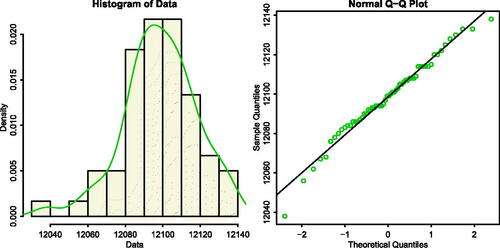
To examine the validity of the normal distribution, several goodness-of-fit statistics and information theoretic criteria are considered, namely: Shapiro and Wilk (1965) normality test, Kolmogorov-Smirnov (KS) with its P-value, AIC and BIC. By computation using shapiro.test built-in package and fitdistrplus library of the R open source software [see, Ihaka and Gentleman (1996)], we have calculated the MLEs of the parameters, which are $\widehat{\epsilon }=12098.5166$ and $\widehat{\varsigma }=19.2306$, where the Shapiro-Wilk test statistic is 0.98032 with P-value being 0.4421, log-likelihood=–262.5265, AIC = 529.0530, BIC = 533.2417, the KS statistic and its P values are 0.0618 and 0.9757, respectively, which suggests that the normal model could fit this data set well. Also, Fig. 3 also supports the normality of the data set.

Fig. 3 Histogram and Q-Q plot of the data set from thickness of membrane of color STN display process.

Data Set II: Voltage of aluminum foil of an electronic company.

This data set is taken from Tong and Chen (2003) and consists of 50 observations of voltage of aluminum foil of an electronic company. The production specifications of the voltage were $(\mathcal{L}, \mathcal{T}, \mathcal{U})=(510, 520, 530)$. If the voltage falls outside this interval, the aluminum foil will break, and thus will be rejected. The data are:

519.9, 519.5, 520.1, 517.0, 521.1, 517.1, 518.7, 520.1, 521.2, 521.7, 520.4, 517.9, 522.9, 517.7, 517.2, 520.7, 521.0, 519.1, 518.4, 518.9, 517.9, 518.4, 520.8, 519.3, 520.6, 516.6, 519.0, 520.6, 517.9, 519.6, 519.6, 522.6, 518.3, 522.1, 523.1, 519.9, 519.8, 520.7, 516.5, 521.5, 519.2, 521.2, 518.9, 517.8, 521.3, 521.3, 517.4, 519.5, 522.0, 523.8

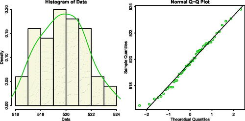
To examine the validity of the normal distribution, several goodness-of-fit statistics and information theoretic criteria are considered, namely: Shapiro and Wilk (1965) normality test, Kolmogorov-Smirnov (KS) with its P-value, AIC and BIC. By computation using shapiro.test built-in package and fitdistrplus library of the R open source software (see, Ihaka and Gentleman 1996), we have calculated the MLEs of the parameters, which are $\widehat{\epsilon }=519.7560$ and $\widehat{\varsigma }=1.7658$, where the Shapiro-Wilk test statistic is 0.98462 with p-value being 0.7551, log-likelihood =–99.37723, AIC= 202.7545, BIC = 206.5785, the KS statistic and its p values are 0.0733 and 0.9505, respectively, which suggests that the voltage data of the aluminum foil fits well for normal model. Also, Fig. 4 supports the normality of the data set.

Fig. 4 Histogram and Q-Q plot of the data set from voltage of aluminum foil of an electronic company.

In summary, from Tables 8 and 9, it is observed that the CME performs marginally better than all other considered methods of estimation for both ${\mathcal{C}}_{\mathit{pmc}}^{\prime }$ and ${\mathcal{C}}_{\mathit{pmc}}$. Further, it is observed that ${\mathcal{C}}_{\mathit{pmc}}^{\prime }$ performs better than their counterparts for Data set I. In addition, it is observed that the width of CI of $\mathcal{B}\mathcal{C}\mathcal{A}\mathcal{B}$ method is smaller than its counterparts among all BCIs. Besides, the MPSE has smaller AW than its counterparts among all classical methods of estimation in terms of the width of BCIs. Besides, the width of ${\mathcal{C}}_{\mathit{pmc}}^{\prime }$ performs better than ${\mathcal{C}}_{\mathit{pmc}}$ in case of MPS method. In addition, we notice that the value of both ${\mathcal{C}}_{\mathit{pmc}}^{\prime }$ and ${\mathcal{C}}_{\mathit{pmc}}$ turns out to be greater than 1 and the process is capable for Data set I.

6 Concluding remarks

In this present study, five BCIs ($\mathcal{S}\mathcal{B},\mathcal{P}\mathcal{B}$, $\mathcal{S}\mathcal{T}\mathcal{B},\mathcal{B}\mathcal{C}\mathcal{P}\mathcal{B}$ and $\mathcal{B}\mathcal{C}\mathcal{A}\mathcal{B}$) of the proposed loss and tolerance cost based PCI ${\mathcal{C}}_{\mathit{pmc}}^{\prime }$ by using six discussed estimation methods for the normal distribution have been considered. Further, we have obtained point estimates of the ${\mathcal{C}}_{\mathit{pmc}}^{\prime }$ using considered methods of estimation. It is to be noted that it would be a tedious task to compare all these considered methods theoretically, hence we have conducted an extensive simulation study to compare these methods with different sample sizes and different combinations of the unknown parameters. In addition, the PCI ${\mathcal{C}}_{\mathit{pmc}}$ is also taken into consideration in real data analysis for comparison purposes. The performances of BCIs for the index ${\mathcal{C}}_{\mathit{pmc}}^{\prime }$ are compared in respect of AW and CPs. Results from the simulation study indicate that $\mathcal{B}\mathcal{C}\mathcal{A}$-boot CIs perform better than their counterparts in respect of AW and CPs for all estimation methods considered in this paper. Also, MLE performs marginally better than considered methods of estimation. The data analysis shows a similar pattern of results that we have observed in the simulation study. As a future research, the proposed PCI, ${\mathcal{C}}_{\mathit{pmc}}^{\prime }$ can be extended in the development of inspection plans and control charts. It can also extended to multivariate versions for the PCI. We hope our results and methods of estimation and BCIs may help companies in using better methods of obtaining the PCIs and their estimations.

Authors’ contributions

The author read and agreed to the published version of the manuscript.

Acknowledgments

The authors truly appreciate the valuable comments from two anonymous Referee which led to an improvement of our work.

Data availability statement

All data analyzed during this study are included in this published articles: Chen and Chen (2004) and Tong and Chen (2003). The link of the data sets used in this study are included within the article, and data sets are also provided in the article.

Disclosure Statement

The author declare that he has no conflict of interest.

Additional information

Funding

The work of Professor Park was partially supported by the National Research Foundation of Korea (NRF) grant funded by the Korea government (MSIT) (No. 2022R1A2C1091319).

References

- Abdolshah, M., R. M. Yusuff, T. S. Hong, and M. Y. B. Ismail. 2011. “Loss-based Process Capability Indices: A Review.” International Journal of Productivity and Quality Management 7(1):1–21. https://doi.org/10.1504/IJPQM.2011.037729
- Alomani, G., R. Alotaibi, S. Dey, and M. Saha. 2020. “Classical Estimation of the Index Spmk and its Confidence Intervals for Power Lindley Distributed Quality Characteristics.” Mathematical Problems in Engineering 2020:1–17. Article ID 8974349. https://doi.org/10.1155/2020/8974349
- Basu, S., S. K. Singh, and U. Singh. 2018. “Bayesian Inference Using Product of Spacings Function for Progressive Hybrid Type-i Censoring Scheme.” Statistics 52 (2):345–63. https://doi.org/10.1080/02331888.2017.1405419
- Chan, L. K., S. W. Cheng, and F. A. Spiring. 1988. “A New Measure of Process Capability.” Journal of Quality Technology 20:162–75. https://doi.org/10.1080/00224065.1988.11979102
- Chen, J., and K. S. Chen. 2004. “Comparison of Two Process Capabilities by Using Indices Cpm: An Application to a Color STN Display.” International Journal of Quality & Reliability Management 21 (1):90–101. https://doi.org/10.1108/02656710410511713
- Cheng, R. C. H., and N. A. K. Amin. 1979. “Maximum Product-of-Spacings Estimation with Applications to the Log-Normal Distribution.” Math Report 79-1, University of Wales IST.
- Cheng, R. C. H., and N. A. K. Amin. 1983. “Estimating Parameters in Continuous Univariate Distributions with a Shifted Origin.” Journal of the Royal Statistical Society B 45:394–403. https://doi.org/10.1111/j.2517-6161.1983.tb01268.x
- Dennis, Jr., J. E., and R. B. Schnabel. 1983. Numerical Methods for Unconstrained Optimization and Nonlinear Equations. Englewood Cliffs, NJ: Prentice Hall, Inc.
- Dey, S., and M. Saha. 2018. “Bootstrap Confidence Intervals of the Difference between Two Generalized Process Capability Indices for Inverse Lindley Distribution.” Life Cycle Reliability and Safety Engineering 7:89–96. https://doi.org/10.1007/s41872-018-0045-9
- Dey, S., and M. Saha. 2019. “Bootstrap Confidence Intervals of Generalized Process Capability Index Cpyk Using Different Methods of Estimation.” Journal of Applied Statistics 46:1843–1869. https://doi.org/10.1080/02664763.2019.1572721
- Dey, S., M. Saha, S. S. Maiti, and C.-H. Jun. 2018. “Bootstrap Confidence Intervals of Generalized Process Capability Cpyk for Lindley and Power Lindley Distributions.” Communications in Statistics - Simulation and Computation 47:249–62. https://doi.org/10.1080/03610918.2017.1280166
- Erfanian, M., and B. S. Gildeh. 2021. “A New Capability Index for Non-normal Distributions based on Linex Loss Function.” Quality Engineering 33:76–84. https://doi.org/10.1080/08982112.2020.1761026
- Hsiang, T. C., and G. Taguchi. 1985. “A Tutorial on Quality Control and Assurance.” Annual Meeting on the American Statistical Association, Las Vegas, NV.
- Hsieh, K.-L., and L.-I. Tong. 2006. “Incorporating Process Capability Index and Quality Loss Function into Analyzing the Process Capability for Qualitative Data.” International Journal of Advanced Manufacturing Technology 27:1217–22. https://doi.org/10.1007/s00170-004-2314-1
- Ihaka, R., and R. Gentleman. 1996. “R: A Language for Data Analysis and Graphics.” Journal of Computational and Graphical Statistics 5:299–314. https://doi.org/10.2307/1390807
- Jeang, A., C.-P. Chung, H.-C. Li, and M.-H. Sung. 2008. “Process Capability Index for Off-Line Application of Product Life Cycle.” In Proceedings of the World Congress on Engineering 2008 Vol II, WCE 2008, July 2–4, London, U.K.
- Juran, J. M. 1974. Juran’s Quality Control Handbook, 3rd ed. New York: McGraw-Hill.
- Kackar, R. N. 1986. “Taguchi’s Quality Philosophy: Analysis and Commentary.” Quality Progress 19:21–30.
- Kane, V. E. 1986. “Process Capability Indices.” Journal of Quality Technology 18:41–52. https://doi.org/10.1080/00224065.1986.11978984
- Kao, J. H. K. 1958. “Computer Methods for Estimating Weibull Parameters in Reliability Studies.” IRE Transactions on Reliability and Quality Control, PGRQC-13:15–22. https://doi.org/10.1109/IRE-PGRQC.1958.5007164
- Kashif, M., M. Aslam, G. S. Rao, A. H. Al-Marshadi, and C. H. Jun. 2017. “Bootstrap Confidence Intervals of the Modified Process Capability Index for Weibull Distribution.” Arabian Journal of Science and Engineering 42:4565–573. https://doi.org/10.1007/s13369-017-2562-7
- Kethley, R. B. 2008. “Using Taguchi Loss Functions to Develop a Single Objective Function in a Multi-Criteria Context: A Scheduling Example.” International Journal of Information Management 19:589–600.
- Leiva, V., C. Marchant, H. Saulo, M. Aslam, and F. Rojas. 2014. “Capability Indices for Birnbaum-Saunders Processes Applied to Electronic and Food Industries.” Journal of Applied Statistics 41:1881–1902. https://doi.org/10.1080/02664763.2014.897690
- MacDonald, P. D. M. 1971. “Comment on “An Estimation Procedure for Mixtures of Distributions” by Choi and Bulgren.” Journal of the Royal Statistical Society. Series B (Methodological) 33 (2):326–29. https://doi.org/10.1111/j.2517-6161.1971.tb00884.x
- Naidu, N. V. R. 2008. “Mathematical Model for Quality Cost Optimization.” Robotics and Computer Integrated Manufacturing 24:811–15. https://doi.org/10.1016/j.rcim.2008.03.018
- Pan, J. N. 2007. “A New Loss Function-based Approach for Evaluating Manufacturing and Environmental Risks.” International Journal of Quality and Reliability Management 24:861–87. https://doi.org/10.1108/02656710710817135
- Pearn, W. L., S. Kotz, and N. L. Johnson. 1992. “Distributional and Inferential Properties of Process Capability Indices.” Journal of Quality Technology 24:216–31. https://doi.org/10.1080/00224065.1992.11979403
- Pearn, W. L., Y. T. Tai, I. F. Hsiao, and Y. P. Ao. 2014. “Approximately Unbiased Estimator for Non-normal Process Capability Index CNpk.” Journal of Testing and Evaluation 42:1408–17. https://doi.org/10.1520/JTE20130125
- Pearn, W. L., Y. T. Tai, and H. T. Wang. 2016. “Estimation of a Modified Capability Index for Non-normal Distributions.” Journal of Testing and Evaluation 44:1998–2009. https://doi.org/10.1520/JTE20150357
- Ranneby, B. 1984. “The Maximum Spacing Method. An Estimation Method Related to the Maximum Likelihood Method.” Scandinavian Journal of Statistics 11 (2):93–112.
- Rao, G. S., M. Aslam, and R. R. L. Kantam. 2016. “Bootstrap Confidence Intervals of CNpk for Inverse Rayleigh and Log-Logistic Distributions.” Journal of Statistical Computation and Simulation 86:862–73. https://doi.org/10.1080/00949655.2015.1040799
- Saha, M., S. Dey, and S. S. Maiti. 2018. “Parametric and Non-parametric Bootstrap Confidence Intervals of CNpk for Exponential Power Distribution.” Journal of Industrial and Production Engineering 35:160–69. https://doi.org/10.1080/21681015.2018.1437793
- Saha, M., S. Dey, and S. S. Maiti. 2019a. “Bootstrap Confidence Intervals of CpTk for Two Parameter Logistic-Exponential Distribution with Applications.” International Journal of System Assurance Engineering and Management 10 (8):623–31. https://doi.org/10.1007/s13198-019-00789-7
- Saha, M., S. Dey, and S. Nadarajah. 2022. “Parametric Inference of the Process Capability Index for Exponentiated Exponential Distribution.” Journal of Applied Statistics. 49 (16):4097–4121. https://doi.org/10.1080/02664763.2021.1971632
- Saha, M., S. Dey, and L. Wang. 2022. “Parametric Inference of the Loss based Index Cpm for Normal Distribution.” Quality and Reliability Engineering International 38 (1):405–31. https://doi.org/10.1002/qre.2987
- Saha, M., S. Dey, A. S. Yadav, and S. Ali. 2021. “Confidence Intervals of the Index Cpk for Normally Distributed Quality Characteristics Using Classical and Bayesian Methods of Estimation.” Brazilian Journal of Probability and Statistics 35:138–57. https://doi.org/10.1214/20-BJPS469
- Saha, M., S. Dey, A. S. Yadav, and S. Kumar. 2019b. “Classical and Bayesian Inference of Cpm for Generalized Lindley Distributed Quality Characteristic.” Quality and Reliability Engineering International 35 (8):2593–11. https://doi.org/10.1002/qre.2544
- Saha, M., S. Kumar, S. S. Maiti, A. S. Yadav, and S. Dey. 2020. “Asymptotic and Bootstrap Confidence Intervals for the Process Capability Index Cpy based on Lindley Distributed Quality Characteristic.” American Journal of Mathematical and Management Sciences, 39:75–89. https://doi.org/10.1080/01966324.2019.1580644
- Shapiro, S. S., and M. B. Wilk. 1965. “An Analysis of Variance Test for Normality (Complete Samples).” Biometrika 52:591–611. https://doi.org/10.2307/2333709
- Shu, M. H., C.-H. Wang, and B. M. Hsu. 2005. “A Review and Extensions of Sample Size Determination for Estimating Process Precision and Loss with a Designated Accuracy Ratio. International Journal of Advanced Manufacturing Technology 27:1038–46. https://doi.org/10.1007/s00170-004-2268-3
- Stevens, D., and R. Baker. 1994. “A Generalized Loss Function for Process Optimization.” Decision Sciences 25: 41–56. https://doi.org/10.1111/j.1540-5915.1994.tb00515.x
- Swain, J. J., S. Venkatraman, and J. R. Wilson. 1988. “Least-Squares Estimation of Distribution Functions in Johnson’s Translation System.” Journal of Statistical Computation and Simulation 29 (4):271–97. https://doi.org/10.1080/00949658808811068
- Tong, L., and J. Chen. 2003. “Bootstrap Confidence Interval of the Difference between Two Process Capability Indices.” International Journal of Advanced Manufacturing Technology 21:249–56. https://doi.org/10.1007/s001700300029
- Varian, H. R. 1975. “A Bayesian Approach to Real Estate Assessment.” In Studies in Bayesian Econometric and Statistics in Honor of Leonard J. Savage, edited by L. J. Savage, S. E. Feinberg, and A. Zellner, 195–208. New York: North-Holland.