A heat transfer and friction factor correlation for low air-side Reynolds number applications of compact heat exchangers (1535-RP)

Abstract

In this article, an experimental investigation of the heat transfer and pressure drop of compact heat exchangers with louvered fins and flat tubes was conducted within a low air-side Reynolds number range of 20< Re_Lp < 200. Using an existing low-speed wind tunnel, 26 sample heat exchangers of corrugated louver fin type, were tested. New correlations for Colburn factor j and Fanning friction factor f have been developed using eight nondimensional parameters based on the experimental data. Within the investigated parameter ranges, it seems that both the j and f factors are better represented by two correlations in two flow regimes (one for Re_Lp = 20 – 80 and one for Re_Lp = 80 – 200) than single regime correlation in the format of power-law. The results support the conclusion that airflow and heat transfer at very low Reynolds numbers behaves differently from that at higher Reynolds numbers.

Introduction

Compact heat exchangers are widely used in commercial and residential air-conditioning (AC) systems. These heat exchangers with multi-louver fins and flat tubes typically have oval tube minor dimensions from 0.8 to 3 mm. This type of design offers several advantages to reducing air-side thermal resistance (Webb and Jung 1992): (1) smaller wake region behind the tube thus not reducing heat transfer downstream; (2) lower profile drag due to smaller projected frontal area of flat tube versus conventional round tube; (2) overall increased air-side heat transfer coefficient and conductance value.

Reducing the air-side thermal resistance, by use of multi-louver fins and flat tubes, for air-cooled heat exchangers can effectively improve performance. A literature survey shows that the available heat transfer and friction factor correlations for louvered surfaces in literature are only valid at high Reynolds number based on louver pitch L_p, Re_Lp > 100. At low Reynolds number (Re_Lp < 100), a concise and accurate correlation is not available. As energy efficiency becomes more and more important in buildings, this type of data for compact heat exchanger is urgently needed to help facilitate the design of more effective commercial and residential AC systems. This need is also driven by the design of low-noise heat exchanger and microchannel heat exchanger (MCHX) that are operated at low airflow rates. In addition, the development of heat transfer and friction factor correlations can provide engineers a better physical understanding of the role of louver dimensions associated with the flow and thermal transition phenomena at low Reynolds numbers.

Compact heat changers with louvered fins have been investigated extensively in the past. Researchers have carried out both experimental and computational studies to understand the underlying fluid flow and heat transfer characteristics. For heat exchanger designs, the performance data, such as Fanning friction factor f and Colburn factor j, for the louvered surfaces have become widely available over the last 25 years. Most of the useful correlations were obtained by experimental methods. Davenport (1983), Achaichia and Cowell (1988), Sunden and Svantesson (1992), Webb and Jung (1992), and Chang et al. (1994) have all performed experiments to quantify performance for louvered fin surfaces of compact heat exchangers. A monumental study was undertaken by Chang and Wang (1997) to consolidate all of the previous test data for generating a generalized heat transfer correlation. This correlation for j- and f-factors is referred to as the Chang and Wang correlation, and is currently the most widely used correlation for predicting air-side resistance and pressure drop for heat exchangers with louvered fins. Kim et al. (2003) has since conducted an additional study for dry and wet surfaces and developed newer j- and f-factor correlations; however, these were based on a much smaller data set and parameter range. Recently, Dong et al. (2007) investigated the multi-louvered fin and flat tube heat exchanger and developed general correlations for both j- and f-factors using larger ratio of fin-to-louver pitches F_p/L_p as compared to that by Kim and Bullard (2002).

Table 1^{Table NaN}shows the f and j correlations developed in the past by various researchers. As can be seen from the table, the number of parameters used in the correlations varies from researcher to researchers. Never the less, most of the correlations for j- and f-factors are in the format of power-law.

Table 1 Existing correlations.

Authors	Correlations	ReLp	Comments
Davenport (1983)		300–4000	f developed for Re = 70–4000. Lh is louver height.
Achaichia and Cowell (1988)		150–3000	Plate-and-tube louver fin. T is tube transverse pitch. St is Stanton number. Four data points when Re < 150.
	f = 0.895f^1.07AFp^− 0.22L^0.25pT^0.26Lh^0.33,fA = 596Re^(0.318logReLp − 2.25)Lp for 50 < ReLp < 3000
	f = 10.4Re^− 1.17LpFp^− 0.05L^1.24pLh^0.25T^0.83 for ReLp < 150
Chang et al. (1994)		100–700	Finning factor, ϵ = Ao/Ato: 7–12
Chang and Wang (1997)		100–3000	91 samples. Tp is tube pitch. f not provided.
Chang et al. (2000)	f = f1*f2*f3	<5000	j not provided.
Kim and Bullard (2002)		100–600	45sample. Fp/Lp<1. TP is tube pitch.

Table

Jacobi et al. (2005)		40–370	a, b, c, d depends on specimen. jChang&Wang is the j proposed by Chang and Wang (1997).
Dong et al. (2007)		200–2500	Fp/Lp > 1
Li and Wang (2010)		400–1600	7 samples. Multi-region louvers. La = 28^o, Lp = 1.2, Fp = 2.8 mm. N is number of louver regions. Re is Reynolds number based on De, a hydraulic diameter.
Li et al. (2011)		200–1730	11 samples. Dc was not defined, but seems Dh, the hydraulic diameter.

A careful evaluation of the previous research indicates that the existing correlations about the j- and f-factors are valid for high Reynolds numbers in the range of 100 to 1000. Jacobi et al. (2005) have proposed a modified j-factor correlation (as compared to that by Chang and Wang 1997) designed to account for curve changing at low Reynolds numbers and recognize optimal louver-fin-pitch design. This correlation was based on test data within a Reynolds number range from 40 to 370; however, the data available for the lower Re_Lp range was very limited (2–3 data points when Re_LP < 100 depending on test samples). In addition, the focus of Jacobi et al. (2005) was to generate a single range correlation. A friction factor correlation was also not proposed. Another example of previous study is Aoki et al. (1989), where very limited data points were used in low Re_Lp range. Within a range of Re_Lp = 60 – 700, their heat transfer data are correlated in terms of Nusselt number (Nu) in a power law format: Nu = 0.87Re_LpPr^1/3, when F_p = 1 mm and θ = 35^o. However, within the range of Re_Lp < 100, only two data points are available.

The lack of credible correlations, for example, j- and f-factors, in the low Reynolds number range is further complicated by the fact that heat transfer and pressure drop are much more sensitive at lower airflow rates than higher airflow rates. At low Reynolds numbers, it has been discussed by several researchers that there might be a transition regime from louver directed to fin directed flow (Hiramatsu et al. 1990; Sahnoun and Webb, 1992). This transition depends on both the Reynolds number and geometrical parameters, such as ratio of fin pitch to louver pitch, F_p/L_p. In general, when Re_Lp is low and F_p/L_p is high, the gap between adjacent louvers is blocked, and the flow is fin directed in the direction of the fin. At higher Re_Lp and lower F_p/L_p the boundary layers are thinner, and the flow is almost aligned with the louvers. However, this phenomenon is not well captured by any of the existing correlations.

It should be pointed out that the concept of two regimes, for example fin directed flow and louver directed flow, has been a controversial subject in the literature. Davenport (1980) conjectured that a flattening behavior (actually “nonpower-law” in their work) of the experimental Stanton number curve as Reynolds number was reduced, was due to this same two-regime effect. Since it was reported, it has been a subject discussed and argued by researchers from different angles (Achaichia and Cowell 1988). For example, Shah and Webb (1983) argued that such flattening or nonpower-law behavior of the Stanton number curve is due to experimental error. Therefore, a new experimental study of heat transfer and pressure drops using specifically instrumented facilities is required to advance the state-of-the-art.

To address the current and future needs in HVAC industries, a detailed experimental study was carried out by the authors to investigate the heat transfer and pressure drop characteristics of compact heat exchangers with louvered fins and flat tubes at different low air-side Reynolds numbers (20 < Re_Lp < 200). The main objective of this research was to develop air-side heat transfer and pressure drop correlations, in terms of j- and f-factors, for high performance compact heat exchangers specifically under low air velocity conditions or within a low Reynolds number range that has not been well investigated.

Compact heat exchangers

The test samples were brazed aluminum microchannel heat exchangers (MCHX) with flat tube louvered fin geometry, similar to the ones tested by Chang et al. (1994).

Figure 1 depicts the definitions of the key geometrical parameters for the flat tube, louver, and fins, as well as the MCHX assemble. Although other types of louver fin heat exchangers as reported in Chang and Wang (1997), this project focused on the “corrugated louvers” with near triangular or rectangular channels for airflows.

Schematic drawing and geometric parameters of microchannel heat exchanger.

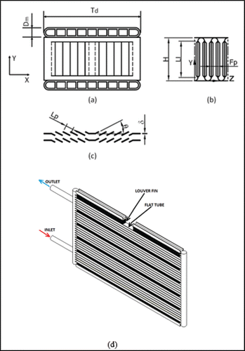
The test samples were commercially available, and were obtained from several manufacturers in the United States, Europe, and Asia who were able to provide the detailed geometries or design drawing of the heat exchangers. Figure 2 is a picture of a typical sample tested in this project. This tested geometry has 18 mm depth of fin array in flow direction, 8.58 mm fin height, 7.11 mm louver length, 27° louver angle, 14 mm fin pitch, and 1.14 mm louver pitch. Test sample core size is 609.4 × 356.8 mm.

A picture of the brazed aluminum heat exchanger sample.

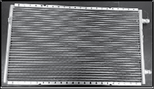
Table 2 Sample matrix.

Sample no.	Fin pitch Fp (FPI)	Fin height H (mm)	Fin thickness δ (mm)	Louver pitch Lp (mm)	Louver angle θ(deg)	Louver length Ll (mm)	Tube height Dm (mm)	Tube depth Td (mm)	Fin depth Fd(mm)	Providers
1	14	8.58	0.13	1.14	27	7.11	1.83	18	18	U1
2	20.3	10	0.1	1.14	25	6.75	1.75	25	25	E1
3	20	8	0.1	0.9	27	6.5	1.5	30	30	E1
4	23	8	0.08	1	28	6.6	1.8	12	12	C1
5	20.3	8	0.08	1	28	6.6	1.8	12	12	C1
6	18	8	0.08	1	28	6.6	1.8	12	12	C1
7	20.3	8	0.1	1	20	6.6	2	16	16	C1
8	23	8	0.1	1	28	6.6	2	16	16	C1
9	21.17	8	0.1	1	28	6.6	2	16	16	C1
10	19.24	8	0.1	1	28	6.6	2	16	16	C1
11	20.3	8	0.1	1	28	6.6	1.8	16	16	C1
12	20.3	7.5	0.1	1	28	6.2	2	16	16	C1
13	14.94	8	0.1	1.3	34	6.6	2	20	20	C1
14	20.3	8	0.1	1	28	6.6	2	20	20	C1
15	20.3	7.5	0.1	1	28	6.2	2	20	20	C1
16	14.94	8	0.1	1	28	6.6	2	26	26	C1
17	20.3	8	0.1	1	28	6.6	2	26	26	C1
18	21.17	5.6	0.1	1	28	6.6	1.4	16	16	C1
19	14	8.00	0.17	1.14	30	5.97	2.03	25.4	25.4	U2
20	12	9.45	0.15	2.44	28	7.87	4.19	26.9	26.9	U3
21	9	9.45	0.15	2.44	28	7.87	4.19	26.9	26.9	U3
22	7	9.45	0.15	2.44	28	7.87	4.19	26.9	26.9	U3
23	11	7.4	0.10	1.02	27	5.97	1.6	25.6	28.0	U5
24	14	7.4	0.10	1.02	27	5.97	1.6	25.6	28.0	U5
25	15	7.4	0.10	1.02	27	5.97	1.6	25.6	28.0	U5
26	18	7.4	0.10	1.02	27	5.97	1.6	26.6	28.0	U5

Table 3 Summary of parameter ranges.

Fin pitch Fp (FPI)	Fin height H (mm)	Fin thickness δ (mm)	Louver pitch Lp (mm)	Louver angle θ(deg)	Louver length Ll (mm)	Tube height Dm (mm)	Tube depth Td (mm)	Fin depth Fd(mm)
7–21.17	5.6–10	0.08–0.17	0.9–2.44	20–34	5.97–7.87	1.5–4.19	12–30	12–30

Table 2 is the test sample matrix developed for this project based on the availability of the MCHXs on the market. A total of 26 heat exchanger samples were used in the test. The test sample matrix covered fairly wide parametric ranges for fin pitch, fin height, fin thickness, louver pitch, louver angle, louver length, tube depth, and fin depth. In place of provider's names, codes were used to maintain confidentiality. The ranges for each parameter are summarized in Table 3.

Test facilities

The heat exchanger samples were tested in an instrumented low-speed wind tunnel in the research laboratory. The wind tunnel has a 0.6096-m long rectangular test section of cross-section 0.635 × 0.457 m on edge. The general design layout of the apparatus is illustrated in Figure 3. The wind tunnel was powered by a 1.5-kW, 1750-RPM centrifugal fan. It provided a maximum speed in the test section (with no blockage) of about 6 m/s and a Reynolds number per meter of up to about 400,000 (based on the tunnel's hydraulic diameter). The tunnel can be operated as a closed loop system or as an open loop by the opening or closing of the loop connect valve or damper (No. 17) as shown the figure. The airflow rate was controlled by changing the inlet and out let dampers (No. 1 and No. 16). Before the test section (No. 10), a flow straightener and an air pre-heater are installed. The original wind tunnel had one circular developing section accompanied with Venturi meter for airflow measurement through the tunnel.

Low-speed wind tunnel apparatus.

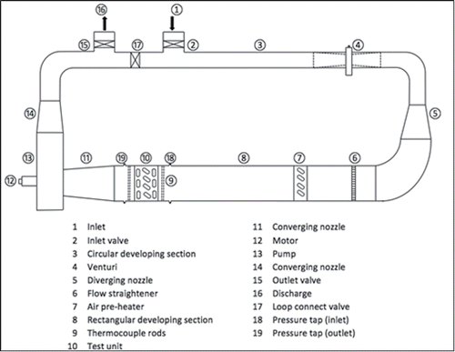
Table 4 Precisions of the measurement instruments.

Parameter	Instrument/method	Range	Precision/error
Air-side temperature	Thermocouple calibration	0–100°C	±0.1°C
Water-side temperature	Thermocouple calibration	0–100°C	±0.1°C
Air-side pressure drop (at test section)	HHP-103 manometer (differential pressure transducer)	0–10.4 in wc (0–2587.9 Pa)	±0.2% FS
Air-side volume flow rate	Orifice: 477A digital manometer	0–335 scfm (0–9.486 m^3/s)	±0.1% FS
	Venturi: 477A digital manometer	260–885 scfm (7.362–25.060 m^3/s)	±0.1% FS
Water-side volume flow rate	FTB-1400 turbine flowmeter	0–7.4 gpm (0–4.668 × 10^-4 m^3/s)	±1%

To facilitate the measurement of the heat transfer and pressure drops at very low Reynolds numbers based on louver pitch (20 < Re_Lp < 200), one venruti meter for relatively higher flow rates, and one orifice meter for relatively lower flow rates, were installed. The working flow rates for each meter were provided in Table 4. On the water-side, the system had a 45-gallon water tank furnished with a standard 4.5 kW heater, as well as a precision tankless heater. The water heater can provide up to 27 kW keeping temperature change less than1^oF. Four pressure taps before and four pressure taps after the test samples, were used for pressure measurement.

Table 4 also provides the summary of the instrumental precisions for the measurement of temperatures, flow rates, and pressure drops on air- and water-sides. A thermocouple grid was applied to measure the air temperatures at inlet (before the heat exchanger) and outlet (after the heat exchanger) to take into account the possibility of nonuniform measurements. T-type thermocouples from Omega Engineering Inc. were used for the measurement of air temperature at inlet and outlet of the test section. Nine thermocouples were used before the heat exchanger and 15 thermocouples were used after the heat exchanger. Less thermocouples were used before the heat exchanger because inlet air temperature is relatively more uniform. On the water-side temperature measurement, T-type thermocouple probes were used at the inlet and outlet, with one on each location, of the connection tubes of the heat exchangers. These thermocouples and probes were pre-calibrated with thermometer of 0.1°C precision. A low-range digital manometer was used to measure the static pressure drop across the test unit during the heating experiment. The operating range of the manometer is between 0 to 2501 Pascal (0 to 10.04 inch H₂O) with accuracy of ±5.002 Pa (0.02008 in. H₂O). The air volumetric flow rate was evaluated from the static pressure difference across the orifice meter as well as the Venturi meter. The pressure difference across the orifice or Venturi meter was measured by digital differential pressure manometer. The operating range of the manometer is between 0 to 4982 Pascal (0 to 20 in. H₂O) with accuracy of ±4.982 Pa (0.02 in. H₂O). Both the orifice and Venturi meters were calibrated by the instrument manufacturers based on National Institute of Standards and Technology (NIST) standards. The water volumetric flow rate was measured using the liquid turbine flow meter. The operating range of the flow meter is between 2.8 to 28 LPM (0.75 to 7.5 GPM) with accuracy of ±1% of reading. The measurements from the turbine flow meter were displayed on 6-digit rate meter. The accuracy of the display is 0.01% of the rate ±1.5 least significant digit (LSD). The flow meter was also calibrated by the manufacture based on NIST standard.

A data acquisition unit was employed to record the transients associated with temperature monitoring of 24 thermocouple junctions on air-side measurements and two thermocouple probes on water-side measurements. The chassis possessed four slots for modules out of which three were used. The calibration standard used for this instrument is ASTM E230-87. Output of the data acquisition unit was fed into a desktop computer via USB-2 interface bus. The personal computer (PC)-based data acquisition system was controlled by LabVIEW software.

For each sample's test, the procedures can be generally divided into the following seven steps: (1) Water was pre-heated. The water in the storage tank was first pre-heated to about 80^oC. This water heating process usually takes about 1 h. (2) The water pump is turned on to circulate the water through the heat exchanger. (3) The fan-motor unit is turned on to move the airflow in the wind tunnel. (4) The control valve is adjusted to achieve the desired airflow rates. (5) Let the system stabilize for about 15–30 min. This is monitored by the data acquisition system to ensure the curves of temperature and pressure versus time are flatting or no noticeable change. (6) Repeat step 4 and 5 for another airflow rate until all data points are collected. Depending on the flow rates, either Venturi or orifice flow meter are to be used. (7) Save data and turn off the system. At least 10 minutes of steady state data, such as inlet and outlet temperatures shown on a stability graph, were required to ensure steady data logging conditions. Stability in the heat exchanger inlet fluid temperature measurement of around 0.02°C per min of sample also means a standard deviation, as suggested by the Electric Power Research Institute (EPRI; 1998). After the system is stabilized, data were recorded for a 30-min test time with 1.1-s interval. Final average values obtained for each temperature as well as pressure drop measurement were used for further data reduction using the procedures to be described in the following section.

The wind tunnel was insulated with fiberglass materials and aluminum tapes. In most of the experiments (over 90%), the energy balance between the water-side and air-side was maintained at less than 5%. At very low Reynolds numbers (Re_Lp < 50), the maximum heat balance was less than 15%. An uncertainty analysis has been performed. In summary, except for cases at extremely low Reynolds numbers or near the lowest end of the instrumental measurement range, reasonable uncertainties can be obtained for j- and f-factors: 91.7% of the uncertainties in the j-factor are less than 7.8%, while 93.0% of the uncertainties in f-factor are less than 7.8%. The maximum uncertainties in j and f-factors are 28.3 and 26.7%, respectively.

Data reduction

The heat transfer rate of the MCHX was computed using the enthalpy method, for both air-side as well as water-side. Air-side heat transfers coefficient was obtained using the effectiveness-number of transfer units (NTU) method. The air-side heat transfer and pressure drop characteristics are presented in terms of Colburn j-factor and friction f-factor, respectively. Air properties were calculated based on ASHRAE Fundamentals Handbook (2013).

The air-side Reynolds number was evaluated based on air properties, minimum free flow velocity of air, and the Louver pitch of the fin as shown in the following Equation 1(1) . (1) Air mass flow rate was calculated using air volumetric flow rate by means of two measuring meters, Orifice meter and Venturi meter, as mentioned earlier. Per ASHRAE Fundamentals Handbook (2013), the volumetric flow rate through the orifice meter in the experiment can be calculated (with simple manipulation) by using the following equation as a function of measured static pressure difference across the orifice (ΔP_ori) installed in the tunnel. (2) where the flow coefficient (K_ori) is a function of discharge coefficient (C_ori) and the beta ratio of the orifice (β_ori). ρ_om is the mean density of the air. Similarly, the volumetric flow rate as a function of measured static pressure difference across the Venturi meter through the Venturi meter (ΔP_ven) installed in the tunnel was estimated using the Equation 3(3) . (3) where the Venturi meter Flow coefficient (K_ven) is a function of discharge coefficient (C_ven) and the beta ratio of the Venturi meter (β_ven).

Repeatability test for sample #1, January 2014.

Repeatability test for sample #13, February 2015.

f and j Factors versus Re_Lp for samples #20, #21, and #22.

f and j factors versus Re_Lp for samples #23 and #24.

f and j factors versus Re_Lp for samples #5 and #6.

f and j factors versus Re_Lp for samples #14 (T_d = 20 mm) and #17 (T_d = 26 mm).

f and j factors versus Re_Lp for samples #12 (T_d = 16 mm) and #15 (T_d = 20 mm).

f and j factors versus Re_Lp for samples #10 (F_p = 19.24 FPI, T_d = 16 mm) and #16 (F_p = 14.94 FPI, T_d = 26 mm).

f and j factors versus Re_Lp for samples #7 (θ = 20^o, D_m = 2 mm) and #11 (θ = 28^o, D_m = 1.8 mm).

f and j factors versus Re_Lp for samples #9 and #25.

The heat transfer rate on water-side as well as air-side was calculated for the test sample through enthalpy method as shown in Equations 4 and 5, respectively. (4) (5) The mathematical average of and was used to calculate the air-side heat transfer coefficient, which is a common practice in existing literature. (6) The maximum possible heat transfer from the heat exchanger based upon hot water and cold air heat exchange system was used for the calculation of the heat exchanger effectiveness. (7) where (8) The effectiveness-NTU method was used to determine the air-side overall heat transfer, UA_o (Incroprea and DeWitt 2000). The UA_o product was calculated using the effectiveness-NTU method for both streams unmixed cross-flow arrangement. Approximate expression for effectiveness-NTU is provided by McQuiston et al. (2005): (9) where (10) (11) (12) For the turbulent flow of water inside the flat tubes, the Dittus-Boelter correlation as expressed in the following Equation 36, was adopted (Incroprea and DeWitt 2000) to evaluate the water-side heat transfer coefficient.The overall surface effectiveness (ϵ_s) can be evaluated from: (13) where (14) (15) The fin efficiency was determined by the method defined in Kays and London (1984). (16) (17) Assuming zero water-side fouling resistance, the air-side heat transfer coefficient was calculated by subtracting the water-side and wall resistances from the total thermal resistance. Therefore, (18) where k_w and δ_w are the thermal conductivity and thickness of the tube wall, respectively. h_i is water-side heat transfer coefficient, which was calculated by the Dittus-Boelter correlations (Incroprea and DeWitt 2000).

Solving Equation 18(18) for h_o yields: (19) The air-side heat transfer characteristic was presented in terms of the Colburn j-factor and can be calculated as follows: (20) where G_c = ρ_omV_c.

Pressure drop equation described by Kays and London (1984), was used to calculate the heat exchanger core Fanning friction factor as follows: (21)

The entrance and exit loss coefficients (K_candK_e) were evaluated for triangular ducts at from Kays and London (1984).

Results and discussions

Repeatability test

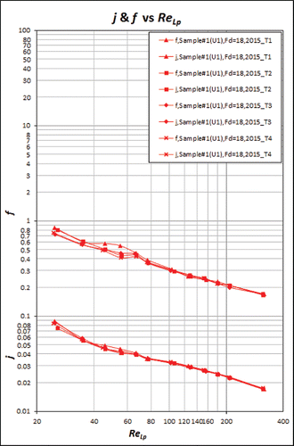
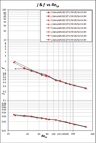
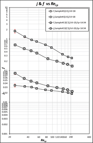
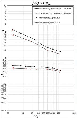
Repeatability tests were conducted at the beginning of experiments and after about every 6 months to verify the measurement instrument stability in the wind tunnel test facility. Figures 4 and 5 show two typical repeatability tests for heat exchanger samples #1 and #13, respectively. In each repeatability test, the experiment was conducted four times with the same conditions. As can be seen from the two figures, the repeatability of the experiments was satisfactory. Except the data in very low Reynolds number range, 90% of the data were within less than 5% of their average value. This provided confidence in the stability of the test facility and instruments during the course of the project period.

f and j factor data

General observations about the j and f factors

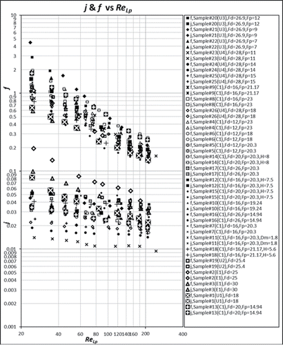
Figures 6–18 provide the j and f factors obtained from the present experimental measurements. In these figures, the experimental data are grouped loosely in a way to try to show the effects of key parameter(s) on the j- and f-factors whenever possible. As discussed below, most of the samples compared in the same figure have more than one variables that are different in value, for example the differences of j- or f-factors for different samples are the combined results of multiple parameters. Of course, this was due to the fact that the test matrix was formed based on available heat exchangers on the market. Only a few heat exchangers were custom-made by the manufacturers due to cost and other restrictions.

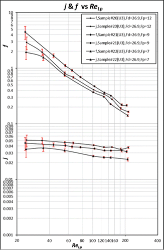
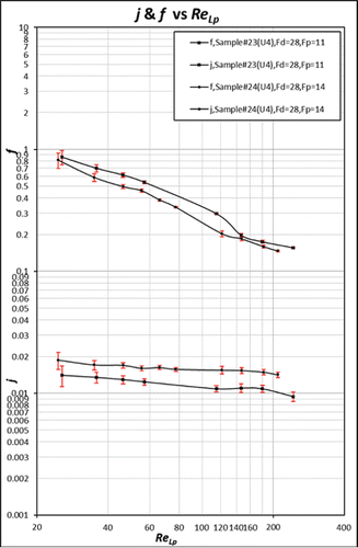
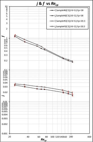
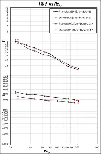
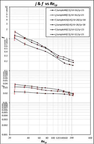
The effects of fin pitch, F_p, on the f- and j-factors are illustrated in Figure 6 (samples #20, #21, and #22), Figure 7 (samples #23 and #24), and Figure 8 (samples #5 and #6). The values of F_p are marked in the figures. These figures cover a fin pitch range of 7–20.3 fins per inch (FPI). In each of these figures, it is clearly shown that, in general, with the increase of fin pitch (increase in FPI or decrease in mm), the magnitudes of both f- and j-factors increase at fixed Reynolds numbers. This is consistent with previous research work in the literature (Chang and Wang 1997; Kim and Bullard 2002). However, the f-factor might not follow this trend for some of the samples. As seen in Figure 7, the f-factor for the lower fin pitch is actually higher, which is consistent with the results reported by Achaichia and Cowell (1988). Such f-factor phenomena may result from the shifting of flow regimes between louver direct flow and fin directed flow due to the complex effects of both geometrical parameters and flow conditions, which need to be further investigated.

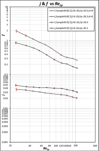
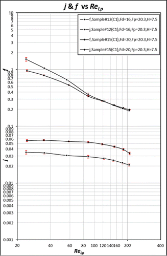
The effects of tube depth, T_d, on the f- and j-factors are illustrated in Figures 9 and 10. In Figure 9, the T_d, values for samples #14 and #17 are 20 and 26 mm, respectively; while in Figure 10 the T_d values for samples #12 and #15 are 16 and 20 mm, respectively. These figures show that with an increase in tube depth, the j-factor increases while f-factor decreases. This seems consistent with some, if not all, of the previous work in the literature (Chang et al. 2000; Chang and Wang 1997).

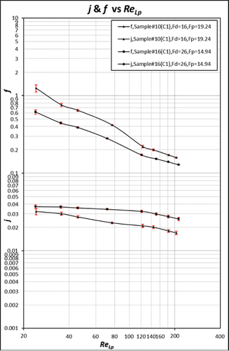
Figure 11 shows the j- and f-factors for samples #10 and #16, where both their tube depth (T_d) and fin pitch (F_p) are different. The tube depth for samples #10 and #16 are 16 and 26 mm, respectively; while the fin depth for samples #10 and #16 are 19.24 and 14.94 FPI, respectively. The combined effect is that sample #10, as compared to sample #16, has higher f and lower j.

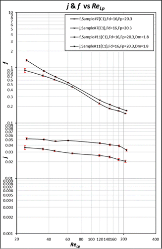
Figure 12 shows the j and f factors for samples #7 and #11, where both their louver angle (θ) and tube height (D_m) are different. The louver angles for samples #7 and #11 are 20^o and 28^o, respectively; while the tube height for samples #7 and #11 are 2 and 1.8 mm, respectively. The combined effect is that sample #7, as compared to sample #11, has lower f- and j-factors.

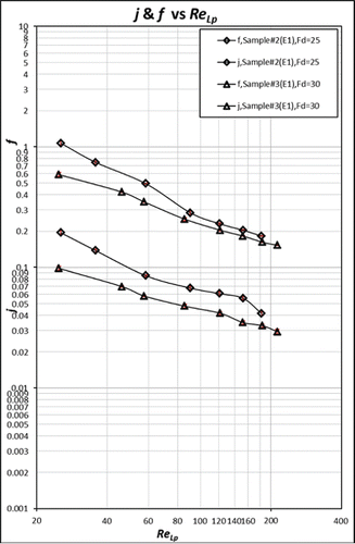
Figures 13 through 17 provide the f- and j-plots for other test samples. As there are more than one geometrical parameters that are varying, the differences in the f- and j-factors in each one of these figures reflected the combined effects of the varying parameters, which are listed in the Test Matrix (Table 2).

All the experimental data are provided in Figure 18, which gives an overview of the data ranges for j- and f-factors within the investigated parameter ranges for this project.

Discussions about the nonpower-law heat transfer phenomena

In the work by Achaichia and Cowell (1988), the heat transfer data, in terms of Stanton number (St, which is proportional to the j-factor), have noticeable “nonpower-law” behavior when the Reynolds number is in very low range (loosely in the order of about Re_Lp < 100 as it depends on samples). In other words, with the increase of Re_Lp, the heat transfer data first drops and then increases within this region in logarithmic scale. The extent of the nonpower-law behavior seems significantly affected by the geometrical parameters, such as fin pitches. This is the region that was sometime claimed as the transition from louver-direct to fin-directed flows. However, such “nonpower-law” behavior was not clearly identified as the dominated characteristics in the heat transfer data obtained from the present project. As will be shown in the next section, only a couple of samples, such as Sample #11 in Figure 12, have shown weak nonpower-law behavior in the present study. In overall, most of the heat transfer test data seem to behave “monotonically” with the change of Reynolds number—with the increase of Reynolds number, the j-factor decreases. It seems the present heat transfer data behave in a way more close to linear relationship with Re_Lp in the logarithmic scale, except that the slopes of the data lines are different from each other in two flow regions (Re_Lp ≤ 80 and Re_Lp > 80). Here, such variation was referred to as the “flattening” phenomena.

Figure 14 f and j factors versus Re_Lp for samples #4, #8, and #26.

Figure 15 f and j factors versus Re_Lp for samples #1 and #13.

Figure 16 f and j factors versus Re_Lp for samples #2 and #3.

Figure 17 f and j factors versus Re_Lp for samples #18 and #19.

It should be also be noted in the differences between the types of heat exchangers used in the present study and those in Achaichia and Cowell (1988), although they all called microchannel or compact heat exchangers with louvered fins. Per the classification by Chang and Yang (1997), the test samples in the present study was type A corrugates louver with triangular channel, while those used in the literature was type B plate-and tube louver fin geometry. The main differences between type A and type B louver fin heat exchangers are:

1. Fins of type A forms triangular channel while fins of type B form parallel plate channel for the airflows.

2. There is usually single flat tube in type A while there are two or multiple flat tubes in type B within the fin depth.

These differences between the type A and type B louver fin heat exchangers could be the main reason that present heat transfer data look somewhat different from previous research in the literature.

Nevertheless, close to half of the test samples in the present study have showed certain levels of flattening phenomena in the j-factors with the decrease of the Reynolds numbers. While some of the test samples have very weak flattening behavior, some other samples, such as those of sample #17 in Figure 9, samples #12 and #15 in Figure 10, and samples #18 and #19 in Figure 17, to name a few, do demonstrate the flattening phenomena that is noticeable in the graphs. This could serve as a confirmation of the existence of unusual or unique characteristics in heat transfer for compact heat exchangers at very low Reynolds numbers. In other words, the two regime concept still can be applied to the present research to explain the heat transfer behaviors in low Reynolds number range.

In summary, it was believed that two flow regimes do exist, where fluid flow and heat transfer behave differently: when Re_Lp is very low (Re_Lp ≤ 80), airflow through the louver is minimized due to thick viscous boundary layers, forming fin directed flow; when Re_Lp is higher (Re_Lp > 80), airflow through the louver is augmented due to thinner boundary layers, forming louver direct flow. The two flow regimes could have different j-behaviors. However, the specific heat transfer curve j versus Re_Lp was dictated by the detailed configurations of the louver fins and flat tubes in the heat exchangers, which might look different from existing work.

These observations provide some guides in developing the power-law correlations for j- and f-factors, to be detailed in the next section.

Correlations for j and f-factors

The collected test data for low Reynolds numbers were analyzed to develop correlations for both the j- and f- factors using all of the key parameters in the text matrix, except the tube depth (T_d). This was because for most of the test samples used in this project, the fin depth (T_d) is identical to the tube depth (F_d). Inclusions of either T_d or F_d resulted in nearly the same correlations and coefficients. Therefore, only F_d, rather than both T_d and F_d was used in the development of correlations for the j- and f-factors. It should be noted that no previous study has included both both T_d and F_d. This might reflect the fact that most of the heat exchangers on the market are made with almost the same T_d and F_d. Heat exchangers with considerably different T_d and F_d might affect the forms of the correlations, but are beyond the scope of this research, and may need to be specifically studied.

In developing the correlations, the percentage of the correlated test data dictates the root-mean-square (rms) errors. In the literature for high Reynolds numbers, the percentage used by researchers varied considerably. For example, 83.14% of the test data of f-factor were correlated within ±15% by Chang et al. (2000); 89.3% of the test data of j-factor were correlated within ±15% by Chang and Wang (1997); 94.5% of test data of f-factor were correlated within ±12%, and 91.1% of the test data of f-factor within ±20% by Li and Wang (2010). As will be shown in the followings, roughly 85% of correlated test data were used for developing the j- and f-factor correlations within the full range of Reynolds number, Re_Lp = 20 – 200, in the present study.

As previously mentioned, most of the present test data supports the existence of two power-law curves of different slopes within two sub-ranges: the lower range (Re_Lp = 20 – 80) and the higher range (Re_Lp = 80 – 200). Our efforts of correlating all of the experimental data using a single correlation equation for either j- or f-factors have resulted in unsatisfactory results. In the following sections, the correlations will be presented using the two Re_Lp sub-ranges with 93.6–99.6% confidence levels. The rms error is indicated right under each correlation equation.

j-factor correlations

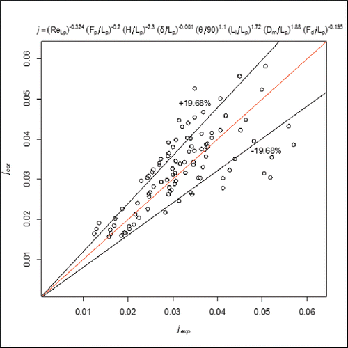
When 20 < Re_Lp ≤ 80, the j-factor can be correlated by Equation 22(22) : (22) The above correlation (Equation 22(22) ) is developed with at least 85.3% of the test data being correlated. Figure 19 shows the comparison of experimental data and the correlation for the j-factors. The present correlation predicts the test data within an rms error of ±19.68%.

Figure 18 f and j factors versus Re_Lp for all samples.

Figure 19 Comparison of experimental data and correlation for j factor (Re_Lp = 20–80).

Figure 20 Comparison of experimental data and correlation for j factor (Re_Lp = 80–200).

Figure 21 Comparison of experimental data and correlation for f factor (Re_Lp = 20–80).

Figure 22 Comparison of experimental data and correlation for f factor (Re_Lp = 80–200).

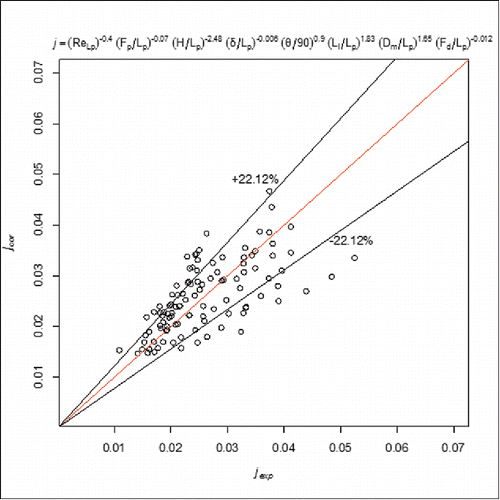
When 80< Re_Lp ≤ 200, the j-factor can be expressed by Equation 23(23) : (23) The above correlation (Equation 23(23) ) correlates at least 84.8% of the test data. Figure 20 shows the comparison of the experimental data and predicted results using the above correlation for the j-factor in the range of Re_Lp = 80–200, within an rms error of ±22.12%.

f-factor correlations

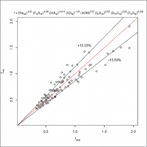
When 20 < Re_Lp ≤ 80, the f-factor can be expressed by Equation 24(24) with at least 85.3% test data correlated. (24) Figure 21 shows the comparison of experimental data and the correlation for the f-factor in the range of Re_Lp = 20–80. The above correlation (Equation 24(24) ) predicts the test data within an rms error of ±13.53%.

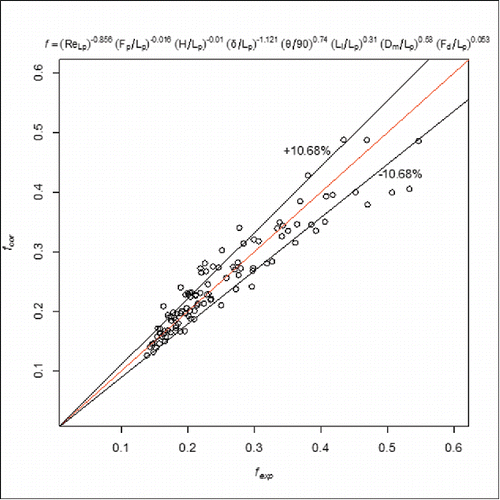
When 80 < Re_Lp ≤ 200, the f-factor can be expressed by Equation 25(25) with at least 85.6% test data correlated. (25) Figure 22 shows the comparison of the experimental data and predicted results using the above correlation for the f-factor in the range of Re_Lp = 80–200. The above correlation (Equation 25(25) ) predicts the test data with an rms error of ±10.68%.

Table 5 Percentage of the total data falling within the specified deviation.

	Deviation of prediction from data
Source of prediction	Within ±5%	Within ±10%	Within ±15%	Within ±20%	Within ±25%	Within ±40%	Within ±45%	Within ±50%
j (Chang and Wang 1997)	7.49%	15.42%	22.03%	28.63%	36.56%	61.67%	69.6%	78.85%
f (Chang et al. 2000)	20.26%	33.92%	47.58%	55.95%	66.96%	92.51%	97.36%	100%
j (Kim and Bullard 2002)	4.41%	12.78%	21.59%	33.48%	44.1%	74.89%	84.14%	92.1%
f (Kim and Bullard 2002)	15.86%	28.63%	38.33%	46.7%	55.07%	82.38%	88.55%	92.95%

Comparison of experimental data with available correlations

In this section, the j- and f-factor experimental data are compared to the well-known correlations by Chang and Wang (1997), Chang et al. (2000), and Kim and Bullard (2002). A summary of the differences between the current data and the correlations by these authors are provided in Table 5.

As can be seen from the previously discussed four correlations, all the correlations by Chang and co-works and Kim and Bullard can only correlate less than 67% (as low as 36.56%) of the current experimental data with a deviation of ±25%. In contrast, as noted earlier, the proposed correlations equations are able to correlate about 85% of the data within errors of less than ±25% (less than ±22.12% for j and less than ±13.53% for f). This confirms that within the investigated parameter ranges, the proposed correlations work better than the existing ones for predicting the test data obtained from this project. This is not surprising as the existing correlations are developed primarily for high Reynolds number applications and the heat exchanger geometries are different from those used in this project. The existing correlations, as reported in the related references, work very well with their own data set, but not for the test data from this project.

Additional comments on the j- and f-factor correlations

First, the fact that the test data can be correlated within two Reynolds number ranges supports the concept of flow regime transition from louver-direct flow to duct-directed flow, to some extent. The existence of the two flow regimes is believed to be the main reason that causes the differences in the correlations in two different Reynolds number ranges, although they are in the same power-law formats.

Second, the signs of the coefficients for every parameter in the power-law correlations are consistent with those reported in most of the literature. However, the absolute values of these coefficients are mostly different from those reported in the literature when power-law formats were used.

Third, a note is also made here that the power-law correlations presented are not perfect. If more test data are to be correlated, the rms errors will further increase, and vice versa. Even with at least 85% test data correlated, the authors believe better correlations with lower levels of rms might be developed by further analysis of the influences of the key parameters or use of different format of mathematical expressions. This could be part of the future work.

Conclusions

In this research project, the heat transfer and pressure drop data for MCHXs are measured on a wind tunnel facility, which was instrumented specifically for low air-side Reynolds number testing in the range of 20 < Re_Lp < 200. Experiments were carried out with 26 aluminum-brazed heat exchanger samples with different designs. The test matrix covered fairly wide geometrical parameter ranges for fin pitch, fin height, fin thickness, louver pitch, louver angle, louver length, tube height, and tube depth.

Within the investigated parameter ranges, it was found that heat transfer relationship, in term of j-factor versus Re_Lp, in low Reynolds range, could be different from that in the high Reynolds range. However, the characteristics of the j-factors versus Reynolds numbers are not exactly the same as reported in the past, which is characterized by a nonpower law behavior. The present heat transfer data are better characterized as a flattening behavior.

Based on the test data, it is possible that the f-factor and j-factor behave as if there are two flow regimes based on the magnitude of Re_Lp. Two sets of corrections have been developed for both f-factor and j-factor in the range of 20 < Re_Lp < 80 and 80 < Re_Lp < 200. The correlations were developed using eight key parameters in the format of power-law. All parameters used in the correlations were nondimensionalized based the louver pitch.

Although power-law formats were used for both j- and f-correlations, the coefficients in each flow regimes were different, reflecting difference in flow and heat transfer characteristics between the relatively lower and relatively higher Reynolds number ranges.

Completion of the present project serves as a good start to fill the knowledge gap in the heat transfer and pressure drop data within low air-side Reynolds number range for design and application of MCHXs using louver fins with flat tubes. However, it should be careful when using the obtained results, as they were based on (and, therefore, more suitable for) the MCHXs of type A corrugated louver with triangular channels. Other types of louver fins might result in different conclusions that need to be investigated.

Acknowledgement

Special thanks are given to members who served on the Project Monitoring Sub-Committee, including Chad Bowers, Stanislav Perencevic, Omar Abdelaziz, Xudong Wang, Joseph Stevenson, Nick Sider, and Mark Johnson, for their very helpful discussions and suggestions during the course of the project.

Funding

The authors would like to express their gratitude to ASHRAE for supporting this research project.

Nomenclature

Ab	=	Air − side surface area of tube, m2
Ac	=	Minimum free flow area, m2
Af	=	Total fin surface area, m2
Afr	=	Frontal area, m2
Ai	=	Water − side total surface area, m2
Ao	=	Air − side total surface area, m2
Aw	=	Tube wall area, m2
C	=	Heat capacity, W/K
cp	=	Specific heat at constant pressure, J/kg.K
Dm	=	Tube height, mm
f	=	Fanning friction factor, dimensionless
Fd =	=	Fin depth, mm
Fp	=	Fin pitch, mm or FPI
FS	=	Full scale
Gc	=	Mass density of air at minimum free flow velocity, kg/m2.sec
H	=	Fin height, mm
h	=	Heat transfer coefficient, W/m2×K
hi	=	Water − side heat transfer coefficient, W/m2.K
j	=	Colburn j-factor, dimensionless
ho	=	Air − side heat trnsfer coefficient, W/m2.K
Kc	=	Entrance loss coefficient
Ke	=	Exit loss coefficient
k	=	Thermal conductivity, W/m×K
kf	=	Thermal conductivity of fin material, W/m.K
kw	=	Thermal conductivity of wall material, W/m.K
lf	=	The fin length, m
Ll	=	Louver length, mm
Lp	=	Louver pitch, mm
	=	Mass flow rate, kg/s
NTU	=	Number of transfer units, dimensionless
Pr	=	Prandtl number, dimensionless
	=	Heat transfer rate, W
	=	Volumetricflowrate, m3/s
R	=	Reference function
	=	Reynolds number based on hydraulic diameter, dimensionless
	=	Reynolds number based on louver pitch, dimensionless
rms	=	Root-mean-square
T	=	Temperature, K
Td	=	Tube depth, mm
UAo	=	Overall thermal conductance, W/K
V	=	Velocity, m/s
Vc	=

Greek Symbols

θ	=	Louver angle, deg.
ΔP	=	Differential pressure, in.wc.
ρ =	=	Density, kg/m3
ρom	=	Air density at bulk mean temperature, kg/m3
δorδf	=	Fin thickness, mm
δw	=	Tube wall thickness; average, m
ϵs	=	Overall surface effectivness, dimensionless
ηf	=	Fin efficiency, dimensionless
ΔP	=	Pressure drop, Pa
ΔT	=	Temperature difference, K
ϵ	=	Effectiveness of the heat exchanger, dimensionless
σ	=	Contraction factor,Ac/Afr
μ	=	Dynamic viscosity, kg/m.s
μom	=	Dynamic viscosity at bulk mean temperature, kg/m.s
νo	=	Viscosity, μom/ρom, m2/s

Subscripts

1	=	Inlet
2	=	Outlet
A/f	=	Area per fin
avg	=	Average
b	=	Base
cs	=	Cross-sectional
d	=	Depth
f	=	Fin
H	=	Height
i	=	Water-side
k	=	Variable
l	=	Length
m	=	Mean
max	=	Maximum
min	=	Minimum
n	=	Number
o	=	Air-side
s	=	Surface
w	=	Wall

Superscript

n

=

Index

References

- Achaichia, A. and T.A. Cowell. 1988. Heat transfer and pressure drop characteristics of flat tube and louvered plate fin surfaces. Experimental and Thermal Fluid Science 1:147–57.
- Aoki, H., T. Shinagawa, and K. Suga. 1989. An experimental study of the local heat transfer characteristics in automotive louvered fins. Experimental and Thermal Fluid Science 1:293–300.
- ASHRAE. 2013. 2013 ASHRAE Handbook—Fundamentals. Atlanta: ASHRAE.
- Chang, Y.-J., K.-C. Hsu, Y.-T. Lin, and C.-C. Wang. 2000. A general friction correlation for louver fin geometry. International Journal of Heat Mass Transfer 43:2237–43.
- Chang, Y.J., and C.C. Wang. 1997. A generalized heat transfer correlation for louver fin geometry. International Journal of Heat and Mass Transfer 40(3):533–44.
- Chang, Y.J., C.C. Wang, and W.R. Chang. 1994. Heat transfer and flow characteristics of automotive brazed aluminum heat exchangers. ASHRAE Transactions 100(2):643–52.
- Davenport, C.J. 1980. Heat transfer and fluid flow in louvered triangular ducts. Ph.D. Thesis, CNAA, Lanchester Polytechnic, Coventry, UK.
- Davenport, C.J. 1983. Correlation for heat transfer and flow friction characteristics of louvered fin. American Institute of Chemical Engineers Symposium Series 79:19–27.
- Dong, J., J. Chen, Z. Chen, W. Zhang, and Y. Zhou. 2007. Heat transfer and pressure drop correlations for the multi-louvered fin compact heat exchangers. Energy Conservation and Management 48:1506–15.
- EPRI TR-107397. 1998. Service Water Heat Exchanger Testing Guidelines. Palo Alto, CA: Electric Power Research Institute Report.
- Hiramatsu, M., T. Ishimaru, and K. Matsuzaki. 1990. Research on fins for air conditioning heat exchangers. JSME International Journal 33:749–56.
- Incroprea, F.P., and D.P. DeWitt. 2000. Fundamentals of Heat and Mass Transfer, 4th Ed. New York, NY: John Wiley and Sons.
- Jacobi, M., Y. Park, Y. Zhong, G. Michna, and Y. Xia. 2005. High Performance Heat Exchangers for Air-Conditioning and Refrigeration Applications (Non-Circular Tubes). Air-Conditioning and Refrigeration Technology Institute, University of Illinois, Urbana, IL. ARTI-21CR/605-20021-01.
- Kays, W.M., and A.L. London. 1984. Compact Heat Exchangers, 3rd Ed. Malabar, FL: Krieger.
- Kim, M.H., and C.W. Bullard. 2002. Air-side thermal hydraulic performance of multi-louvered fin aluminum heat exchanger. International Journal of Refrigeration 25(3):390–400.
- Kim, M.H., S.Y. Lee, S.S. Mehendale, and R.L. Webb. 2003. Microchannel heat exchanger design for evaporator and condenser applications. Advances in Heat Transfer 37:297–429.
- Li, W., and X. Wang. 2010. Heat transfer and pressure drop correlations for compact heat exchangers with multi-region louver fins. International Journal of Heat Mass Transfer 53:2955–62.
- Li, J., S. Wang, and W. Zhang. 2011. Air-side thermal hydraulic performance of an integrated fin and micro-channel heat exchanger. Energy Conversion and Management 52:983–9.
- McQuiston, F.C., J.D. Parker, and J.D. Spitler. 2005. Extended Surface Heat Exchangers, 6th Ed. Heating, ventilating, and air conditioning analysis and design. Hoboken, NJ: John Wiley & Sons, Inc., pp. 482–513.
- Sahnoun, A., and R. Webb. 1992. Prediction of heat transfer and friction for the louver fin geometry. Journal of Heat Transfer 114:893–900.
- Shah, R.K., and R.L. Webb. 1983. Compact and Enhanced Heat Exchangers. Heat exchangers: theory and practice. J. Taborek, G.F. Hewitt, and N. Afghan, eds. pp. 425–68. . New York, NY: McGraw-Hill.
- Sunden, B., and J. Svantesson. 1992. Correlation of j- and f-factors for multi-louvered heat transfer surfaces. Proceedings of the 3rd UK National Heat Transfer Conference, Edgbaston, Birmingham, UK, September 16–18, pp. 805–11.
- Webb, R.L., and S.H. Jung. 1992. Air-side performance of enhanced brazed aluminum heat exchangers. ASHRAE Transactions 98(Pt. 2):391–401.