Detailed velocity profiles in close-coupled elbows—Measurements and computational fluid dynamics predictions (RP-1682)

Abstract

This article presents a systematic study to measure detailed velocity profiles in close-coupled five-gore elbows having nominal diameters of 305 mm (12 in) and turning radii r/D = 1.5, and to, likewise, predict the velocity profiles using computational fluid dynamics. The purpose of the testing was to study the physics of the flow in complex geometries and to provide data that can be used to verify the accuracy of computational fluid dynamics modeling predictions. The close-coupled elbow combinations comprised either a Z-shape or a U-shape configuration. In every instance the duct length separating the center-points of the elbows was systematically varied. Detailed velocity profile measurements were performed at one traverse plane located one duct diameter upstream of the first elbow and at one duct diameter downstream of the second elbow, and at various axial locations in the straight section between the close-coupled elbows. Velocity profiles results are compared to computational fluid dynamics Reynolds Stress Model and Large Eddy Simulation predictions for the effect of separation distance of the elbows in Z-shape duct configurations. Reynolds Stress Model turbulence modeling predicted the velocity trends correctly with a maximum error of 15%. However, Large Eddy Simulation modeling failed to predict the trend and the magnitude of the velocities, thus Large Eddy Simulation approach is not suitable for this type of flow.

Introduction

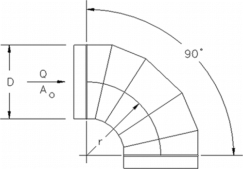
This article presents a systematic study to measure detailed velocity profiles in close-coupled elbows and then to use the experimental data to verify the accuracy of computational fluid dynamics (CFD) modeling predictions. The focus of the testing was to study the physics of flow in complex geometries not studied previously. A test program was initiated to measure the velocity profiles in two close-coupled five-gore elbows with r/D = 1.5; refer to Figure 1. Results from tests conducted on ducts/fittings having a nominal diameter of 305 mm (12 in) are reported. Additional experimental pressure drop data, velocity profile measurements, and CFD predictions obtained for 305 mm (12 in) diameter ducts and fittings are provided in RP-1682 (2015).

Fig. 1. Ninety degree five-gore elbow r/D = 1.5.

Since 1988 there have been several experimental research projects sponsored by ASHRAE, e.g., RP-551 (1991), RP-690 (1994), RP-1319 (2008), RP-1488 (2011), and RP-1606 (2014), designed to populate the Duct Fitting Database (ASHRAE 2015). The results from these studies have been published in the open literature. The pressure loss for flat oval straight ducts has been reported in Townsend et al. (1994). For flat oval tee and lateral fittings, it has been found that branch loss coefficients were Power Law functions of branch-to-common flow rate ratio, and the main loss^{Fig. 1, Fig. 2}coefficients were Power Law functions of the main-to-common flow rate ratio, and generally less than 0.02 at high flow rate ratios; refer to Townsend et al. (1996a), Idem and Khodabakhsh (1999), Idem (2003), Kulkarni et al. (2011), and Gibbs and Idem (2012). Loss coefficient data for flat oval elbows have been expressed as Power Law functions of aspect ratio and hydraulic diameter; refer to Townsend et al. (1996b) and Kulkarni et al. (2009). The goal of RP-1606 (2014) was to evaluate loss coefficients of flat oval to flat oval transitions where the major and minor axes were either concentric or eccentric. Recently RP-1493 (2011) was completed. The primary objective of that project was to ascertain whether CFD could be used to determine loss coefficients for divided flow duct fittings, in the absence of empirical input. The ultimate goal of that effort was to reduce the number of expensive and time-consuming laboratory tests required to enhance the DFDB. The main findings of the project were that the trends of the pressure loss coefficients were predicted correctly, while a CFD prediction accuracy within 15% of experimental data was not achieved. The results of that study are summarized in Sleiti et al. (2013), Liu et al. (2012), Manning et al. (2013), and^{Fig. 1, Fig. 2}Gutovic et al. (2013). Recently, a related study has been published by Salehi et al. (2017a) on identifying CFD models for use in determining HVAC duct fitting loss coefficients. Another experimental and CFD study was published by Salehi et al. (2017a) on pressure loss in close-coupled elbows. An extensive body of literature exists pertaining to either CFD or experimental modeling of pressure loss in single or close-coupled fittings; these references include Gan and Riffat (1995), Mahank and Mumma (1997), Mumma et al. (1997, 1998), Rahmeyer (2002), Sami and Cui (2004), and Mylaram and Idem (2005).

Several research papers in open literature reported experimental measurements of velocity profiles in various shapes of duct geometries. However, detailed experimental velocity profiles in close-coupled Z- and U- configurations ducts have not been studied before. The purpose of this study is to fill the knowledge gap in this area and to provide experimental data that can be used to verify the accuracy of CFD modeling predictions.

Experimental program

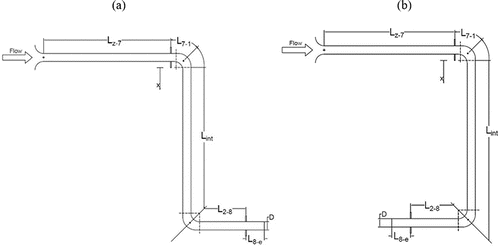
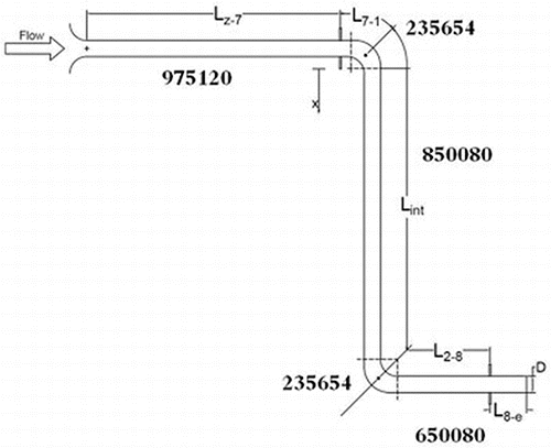
Two close-coupling configurations were studied in the present experiments. Per the terminology employed by Sami and Cui (2004), in one instance the close-coupled test apparatus constituted a Z-shape, whereas in other instances the experiments conformed to a U-shape. These cases are sketched in Figures 2a and 2b, respectively. In each case the straight duct length inserted between the upstream elbow and the downstream elbow was systematically varied; refer to RP-1682 (2015) for further details.

Fig. 2. Test setup. a. double elbow Z-configuration; b. double elbow U-configuration.

In every instance the elbows and ductwork were constructed from 26-gauge galvanized steel. The ducts upstream and downstream of the test section were each 1.20 m (4 ft) in length, and were connected by slip couplings. For close-coupled elbows the intermediate length x, measured from the exit plane of the upstream elbow to the entrance plane of the downstream elbow, was varied from 0 m (0 ft) to 3.05 m (10 ft) in increments of 0.60 m (2 ft); refer to Figures 2a and 2b. For an intermediate length of 0 m (0 ft), the two elbows were butted together, and the joint wrapped tightly by a rubber sheet for mechanical integrity. There were no joints in the intermediate duct mounted between the close-coupled elbows. All joints and fitting connections were thoroughly sealed using cloth-backed tape. A 30 hp centrifugal fan provided air flow through the test apparatus in the forced draft mode. A multiple-nozzle chamber in compliance with the requirements of Standard 120–2008 was used to measure the volume flow rate through the test setup.

For various combinations of close-coupled intermediate section lengths and apparatus configurations (i.e., Z-shape or U-shape), detailed velocity profile measurements were performed using a five-hole directional velocity probe. One traverse plane was located one duct diameter upstream of the first elbow. Another measurement plane was situated one duct diameter downstream of the second elbow. Likewise, detailed velocity profile measurements were performed at various axial locations in the straight section between the close-coupled elbows. The specific locations of the velocity profile measurements are presented in Table 1 as a function of intermediate length (x/D), measured relative to the exit plane of the upstream elbow.

Table 1. Test section velocity profile axial measurement locations.

Intermediate section length (Lint / D)	Measurement location (x/D)
4.36	1
6.40	1,3
8.36	1,3,5
10.42	1,3,5,7
12.40	1,3,5,7,9

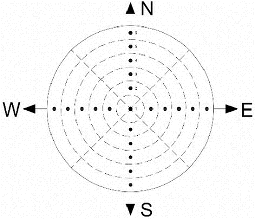
The five-hole probe was first located at the centerline of the duct. Thereafter, the probe was re-positioned in radial increments of 25.4 mm (1 in.) on either side of the centerline; refer to Figure 3. In every instance the sensing tip of the five-hole probe was located with an accuracy of ± 1.25 mm (0.05 in.), relative to the duct centerline. For every traverse performed, air velocities were measured in two mutually perpendicular planes. The two planes divided the cross section of the circular duct into four equal quadrants. The differential pressure measurements required by the directional probe were performed using electronic manometers.

Fig. 3. Velocity radial traverse locations.

A five-hole probe simultaneously measures total pressure in a centrally located port, indicated by p₁, the static pressures p₂ and p₃ in the yaw plane, and pitch angle pressures p₄ and p₅. The relationships between these pressures are expressed as dimensionless coefficients, which are functions of flow angularity. The differential pressure measurements required by the directional probe were performed using electronic manometers having a measurement accuracy of ± 2.5 Pa (0.01 in. H₂O). The first manometer measured the differential pressure from ports 2 and 3. The second manometer measured the differential pressure from ports 4 and 5. A third manometer was used to measure the pressure difference from port 1 and port 2. Once the probe was situated at the desired radial location, it was rotated in the traverse unit until the differential pressure (p₂ −p₃) = 0, as indicated on the manometer. The yaw angle of the flow was then read directly from the scale located on the traverse unit. Thereafter the differential pressures (p₁ −p₂) and (p₄ −p₅) were measured using electronic manometers. Calibration curves provided with the five-hole probe were then used to calculate the pitch angle and velocity magnitude at each location. The pitch angle and velocity pressure coefficients (VPCs) were calculated from calibration curves provided by the probe manufacturer.

Data reduction for the five-hole probe velocity measurements closely followed that outlined in Treaster and Yocum (1979), and is herein summarized. The yaw angle α was measured directly for the condition where p₂ and p₃ were balanced, such that p₂ −p₃ = 0. Thereafter the pitch angle pressure coefficient (PAPC) was calculated from the following equation: (1)

The flow pitch angle β was obtained from the factory calibration curve, where the PAPC is plotted as a function of pitch angle. The VPC is likewise defined as follows: (2)

The measured pitch angle in turn was used to calculate the VPC from a factory calibration curve where the VPC is plotted as a function of pitch angle. The product of VPC and differential pressure p₁ – p_2,3 yields the velocity pressure p_t – p_s. Hence, the magnitude of the velocity vector approaching the probe sensing element is given by: (3)

The air velocity measured at a point can be resolved into three velocity components, oriented with the axial, radial, and circumferential coordinates of the pipe. For example, the flow component oriented parallel to the flow axis in the scale model test section is given by: (4)

Velocity profile mass balances

In order to verify that mass conservation was achieved for each measured axial velocity profile the following analysis was performed. Fundamentally the volume flow rate at any axial location was obtained by integrating the velocity measured at each radial location over the cross-section of the duct as follows: (5)

In one quadrant Equation 5(5) can be approximated by the following expression, which is derived based on the trapezoidal rule of numerical integration: (6)

In this instance V_i represents the measured axial velocities at each radial location r₁, r₂ , …, r₆, and it is understood that r₁ = 0 and = 0 at r = r_o. This expression can be simplified algebraically such that in a single-duct quadrant: (7)

Therein, the total volume flow rate at each cross section was obtained by summing over each of the four quadrants: (8)

Likewise, the mean air velocity in the duct at any axial location was calculated using: (9)

CFD approach

In this study, two advanced turbulence modeling approaches were used and compared; the Reynolds Stress Model (RSM) and the Large Eddy Simulation (LES). The RSM has the capability to accommodate high Reynolds number turbulent flows, which is a great advantage over one and two equation models. It is necessary to adopt a second moment closure model when simulating stress induced secondary flows in ducts. The boundary conditions of RSM require user-defined Reynolds stresses and dissipation rate. This model is general but is complex when compared to other turbulence models. The model has six transport equations for Reynolds stresses and an equation for the dissipation rate ϵ, the model equation is as follows (ANSYS 2009): (10)

The terms on the right represents the dissipation, the redistribution, the turbulent transport, the production and the molecular viscous transport. The last term is a closed term since it contains only the dependent variable and the mean flow gradients.

LES is a multi-scale technique with a complexity intermediate between Direct Numerical Simulation (DNS) and the Reynolds Averaged Navier-Stokes (RANS) approaches. The LES approach separates the multiple turbulent scales, where large, energy-containing eddies are directly computed while small-scale turbulent structures are assumed to be uniform and are, therefore, considered for modeling. The small scales are more likely to be homogeneous and isotropic than the larger scales and as a result, are more appropriate for universal modeling. In addition, the modeled subgrid scale stresses only contribute in a little portion of the whole turbulent stresses.

The basis of separation between the small and large scales relies on a filtering procedure with a filtering function G. The filter removes all finer fluctuations and the governing equations only describe the space-filtered fields. The instantaneous flow field is split to resolved large scales () and also modeled small scales (ϕ′), as follows: (11)

The extraction of the resolved large scale part from the original variables is mathematically defined by the convolution of the original variables with a filter function. The filtering operation of the governing equations results in additional subgrid-scale stress terms: (12) which represents the relations between the resolved large scale and the unresolved small scale part of the flow. The problem of turbulent closure is the expression of these unknown contributions in terms of the resolved large scale quantities. Thereby, subgrid-scale models are used to simulate energy transport between the resolved and unresolved parts.

Numerical simulation details

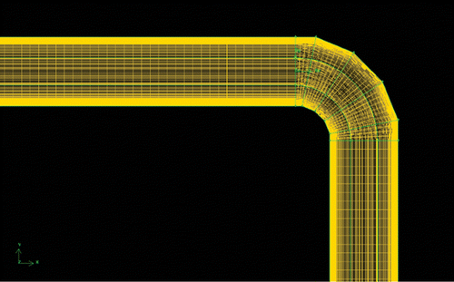
The CFD simulations were conducted using ANSYS Fluent. The three-dimensional (3D) geometry and numerical grid were both generated using ANSYS. Different mesh schemes were conducted and the first mesh adopted was an unstructured grid which caused reversed flow in the duct and led to unrealistic results. Therefore, a structured grid was used for all simulations reported in this article. The mesh was finer near the bend region where there will be flow detachments and recirculation zones. A Grid Independence Study (GIS) was performed and coarser grids were refined and analyzed for viscous sublayer y+ at walls and velocity magnitude. To achieve a structured mesh along the model, a mapped face meshing quadrilaterals method was adopted. Adjustments had to be made to the geometry, by slicing the whole body into different parts to allow flexibility in modelling the part, and to increase the number of elements in the bend region. Four edge sizing was used to obtain the desired mesh and to possibly increase the number of elements near the walls using a variable bias factor.

Near-wall treatment

It is significantly important for turbulence modeling to consider that near-wall flow is affected by damping, and, therefore, velocity is decreased. The concave wall is affected by kinetic energy caused by a sudden increase in velocity. The flow has to be defined correctly near the wall region to satisfy turbulence modelling. Normally the RSM model performs better with flows away from walls. There are three layers near the wall, including a viscous sublayer which is a laminar flow and falls in the y⁺ < 5 near the wall region. The range from 5 < y⁺ < 30 is the buffer layer in which transition occurs. From 30 < y⁺ < 1000 is the log or fully turbulent layer. Above y⁺ = 1000 is the outer region and a wake is present.

In order to simulate flows near the boundary layer, wall functions must be used. They act as a connection between laminar and fully turbulent flows. A wall function approach is appropriate when used in conjunction with high Reynolds number values. Another approach could be implemented where the near-wall mesh is refined to achieve the desired near-wall region y⁺. Each turbulence model has its own configuration in terms of y⁺ values. Approximations of velocity profile shapes could be presented in terms of u⁺ and y⁺: (13)

In this instance u_τ is the friction velocity that can be used to approximate the y⁺ parameter. In this article, to ensure that results are independent from near-wall region characteristics, a near-wall treatment was adopted in RSM with a y⁺ < 1. This is computationally demanding and requires extra computational time to solve; however, results should be accurate and stable.

GIS

A GIS was performed for several cases to determine the suitable numerical grid that will result in y⁺ in the order of unity. Representative results are shown in Table 2.

Table 2. Grid independence study.

	Number of elements	y+ min	y+ max	y+ avg
Course	318,000	0.1381	0.7464	0.4244
Medium	440,000	0.1003	0.7613	0.4264
Fine	511,000	0.3288	0.7909	0.4263

From Table 2, it can be seen that there is small variation from one grid to another in the value of maximum y⁺. Comparing the course and fine grids, there is a large variation which exceeds the tolerance. Therefore, the medium grid could be adopted as it is within a tolerance range of less than 4% in the maximum y⁺ values. It has around 70,000 less elements than the fine mesh and it will greatly save computational time.

Boundary conditions

At the entrance the inlet velocity boundary condition was used. The outlet was defined by pressure outlet boundary conditions. The pressure outlet was selected as it has better convergence results than velocity outlets in models where backflow exists. The wall boundary condition was set to the no-slip condition. The solid-wall was set with a constant roughness value of 0.0009, which was measured experimentally as reported in ASHRAE RP-1682. Similar to the experimental measurements, the CFD model required that the flow at inlet was fully developed before it entered the bend. The convergence of solutions was based on the residual value of velocities. With appropriate under-relaxation factors, the solution obtained was converged and stable.

Experimental results

For various combinations of close-coupled intermediate section lengths between the mid-point of the upstream elbow and the mid-point plane of the downstream elbow, i.e., , and for both the Z- and U-configurations, detailed point velocity profile measurements were performed along two perpendicular radial directions using a five-hole directional velocity probe on the 305 mm (12 in) diameter test apparatus as previously described. The measurements were nominally performed at a single Reynolds number. However due to small variations in ambient conditions that occurred throughout the test program the Reynolds numbers for the velocity profile tests ranged from 3.3 × 10⁵ to 3.6 × 10⁵. The resulting magnitudes of the air velocities in the principal flow direction as calculated using Equation 3(3) are subsequently presented side by side with CFD results for the Z-configuration. In these instances, the N-S direction is parallel to the axis about which the elbow turns. Conversely the E-W axis is perpendicular to the N-S direction, and the plane defined by the N-S and E-W axes is normal to the air flow direction in any section of the apparatus. In every instance the quantity V is normalized by the value recorded at the duct centerline. Likewise, the local radial location where a measurement was performed is non-dimensionalized by the overall duct radius. In these figures the flow direction is out from the page, such that along the N-S axis a radius r/r_o = 1 corresponds to the northernmost measurement location, whereas a value r/r_o = –1 indicated the southernmost position. Likewise, along the E-W axis a radius r/r_o = 1 denoted the easternmost measurement, and r/r_o = –1 signified the westernmost location.

For each value of^{Table 3, Table 4}L_int/D the measured velocity profiles measured one-dimensional (1D) upstream of the first elbow in the close-coupled configurations were typical of fully developed turbulence in both the N-S and E-W traverse directions. For those locations in the test setups the highest momentum/velocity was located at the duct centerline. For both the Z- and U-configurations when there was an intermediate section of duct imposed between the two elbows, there was a velocity deficit in the E quadrant (i.e., the elbow throat) 1D downstream of the first elbow along the E-W traverse. By contrast along the E-W traverse for x/D = 1 there was a velocity surfeit in the W quadrant, i.e., the air had congregated in the heel of the elbow. In the N-S direction the minimum velocities at x/D = 1 for both the Z- and U-configurations (not shown for U-configuration in this article) were located at the center of the duct while the greatest velocities were near the north and south walls. Likewise, for both the Z- and U-configurations, 1D downstream of the first elbow the minimum fluid velocity in the N-S traverse was always present at the duct centerline, further illustrating that as flow occurred around the first elbow the higher momentum fluid initially located along the centerline was pushed to the heel of the elbow, yielding a velocity deficit along the flow axis in all traverse directions.

If^{Fig. 4}the intermediate duct section length was sufficiently long, by x/D = 3 both the N-S and E-W traverses exhibited a local minimum along the flow centerline. A diminishing velocity deficit was observed up to x/D ≅ 7. However, by x/D = 9 the flow began to resemble the fully developed profile observed upstream of the first elbow both in the N-S and E-W traverse directions. These qualitative observations were consistent regardless of the intermediate duct section length, such that the local velocity profiles measured in the N-S and E-W directions depended almost entirely upon distance downstream from the first elbow for the Z- and U-configurations. For the Z-configuration tests, at a measurement location one diameter downstream of the second elbow there was a readily apparent velocity deficit in the E quadrant, which in this instance was the elbow throat. For U-configuration tests a velocity deficit occurred 1D downstream of the second elbow in the W quadrant, which again constituted the throat of the elbow. In both instances there was virtually no corresponding increased velocity in the heel region of the elbow. Interestingly, for both the Z- and U-configurations the measured velocity profiles in the N-S directions were virtually flat over the entire traverse direction 1D downstream of the second elbow. Once again, these qualitative observations were essentially independent of the intermediate duct section length.

Due to the inability of the five-hole velocity probe to readily measure air velocity in the presence of flow reversal when oriented into the flow direction, a mass conservation analysis was performed at each axial location in the test section. In that case the average velocity 1D upstream of the first elbow was evaluated numerically by means of Equation 9(9) . This location was chosen because it was deemed that the velocity profile at that location exhibited characteristics of fully developed turbulence, indicating a lack of flow reversal/separation, and could therefore be accurately measured. Thereafter the average air velocity at each of the downstream axial locations was likewise measured by numerically integrating each traverse over the duct cross section using Equation 6(6) . The intent was to verify that although the flow downstream of the first elbow exhibited considerable swirl, for x/D ≥ 1 there was no apparent flow reversal. Therein a ratio of average velocity at each axial location in the test section to that upstream of the first elbow was calculated. These results are presented in Tables 3 and 4. At all^{Fig. 4}traverse locations it was found that . This strongly implies that the average velocity at each axial location in the test section was measured with an accuracy of ± 4%, and that mass conservation was achieved. There was no discernible flow reversal for x/D ≥ 1 either for Z- or U-configuration velocity profile measurements. The absence of flow reversal downstream of either elbow was further confirmed in the experimental program simply by rotating the five-hole velocity probe by 180° in those regions where flow reversal was suspected, such that sensing ports of the probe then pointed in the overall flow direction. These efforts verified the nonexistence of flow reversal and further substantiated the velocity profile measurements.

Table 3. Z-configuration mass balance comparison at test section axial locations.

		x/D
Lint / D	Upstream elbow	1	3	5	7	9	Downstream elbow
2.36	1.000	—	—	—	—	—	0.998
4.36	1.000	0.984	—	—	—	—	1.000
6.40	1.000	0.980	0.990	—	—	—	0.996
8.36	1.000	0.984	0.984	0.984	—	—	0.983
10.42	1.000	0.996	0.993	0.994	0.993	—	1.009
12.40	1.000	0.985	0.981	0.996	0.984	0.996	0.988

Table 4. U-configuration mass balance comparison at test section axial locations.

		x/D
Lint / D	Upstream elbow	1	3	5	7	9	Downstream elbow
2.36	1.000	—	—	—	—	—	0.982
4.36	1.000	0.974	—	—	—	—	0.965
6.40	1.000	0.982	0.985	—	—	—	0.975
8.36	1.000	0.985	0.982	0.990	—	—	0.966
10.42	1.000	0.986	0.991	0.987	0.994	—	0.969
12.40	1.000	0.975	0.981	0.989	0.989	0.991	0.971

CFD results

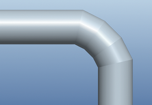
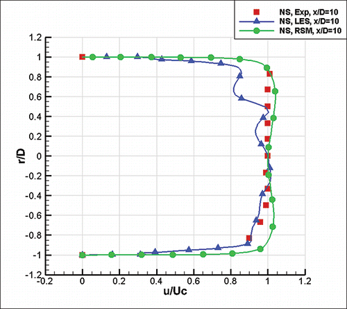
In this section the RSM and LES turbulence models are investigated for their ability to predict the velocity profiles for six different duct locations namely, at x/D = 1, 3, 5, 7, 9, and outlet for the 305 mm (12 in) duct diameter Z-configuration pipe with a separation distance ratio of 10 between the 90° elbows. The geometry of the five-gore elbows used in all simulations is illustrated in Figure 4. The mesh consisted of approximately 2 million cells, and at least 12 grid points were placed in the boundary layer next to the wall. Mesh sizes smoothly increased away from the walls; refer to Figure 5a. The number of finite volumes for each section of the Z-configuration duct are shown in Figure 5b.

Fig. 4. Geometry including the five-gore elbow.

Fig. 5a. Mesh generation of the geometry.

Fig. 5b. Number of finite volumes in each section of the geometry.

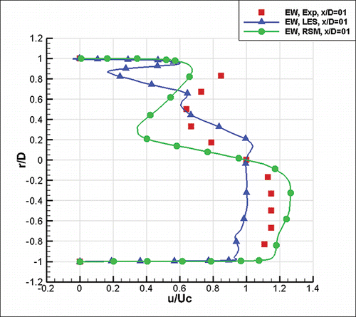
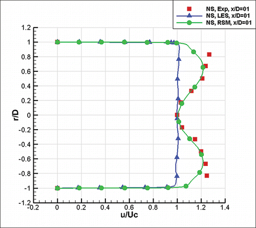
At x/D = 1, RSM predicted the velocity trends correctly as shown in Figures 6 and 7 for both the E-W and N-S directions. However, the difference in experimental and CFD-RSM velocity magnitudes peaked at approximately 15% at r/D = 0.3 in the E-W direction (Figure 6), while the error was less than 3% in the N-S direction (Figure 7). This suggests that the velocity deficit in the E quadrant (i.e., the elbow throat) 1D downstream of the first elbow along the E-W traverse was not predicted accurately by RSM. By contrast along the E-W traverse for x/D = 1 where there was a velocity surfeit in the W quadrant, i.e., the air had congregated in the heel of the elbow, RSM predictions were accurate to within 6%. In the N-S direction 1D downstream of the first elbow where the minimum fluid velocity in the N-S traverse was always present at the duct centerline and where the higher momentum fluid initially located along the centerline was pushed to the heel of the elbow, RSM predicted the velocities with a maximum error of 3%. On the other hand, LES modeling failed to predict the trend and the magnitude of the velocities.

Fig. 6. Comparison of RSM and LES models against experimental data at x/D = 1 (E-W).

Fig. 7. Comparison of RSM and LES models against experimental data at x/D = 1 (N-S).

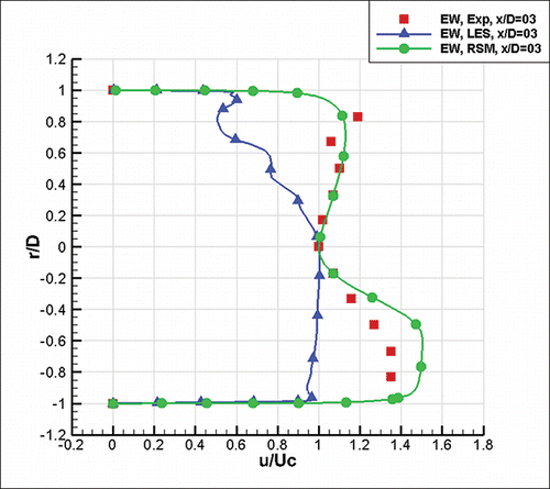
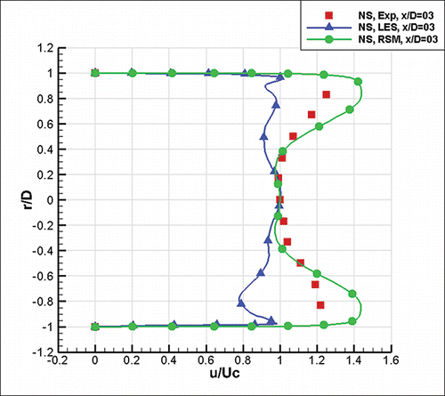
At x/D = 3, RSM predicted both the velocity trends and magnitudes correctly as shown in Figures 8 and 9 for E-W and N-S directions, respectively. The difference in experimental and CFD-RSM velocity magnitudes peaked to about 10% at r/D = –0.5 in the E-W direction (Figure 8), while the error was less than 8% in the N-S direction (Figure 9). However, once again the LES modeling failed to predict the trend and the magnitude of the velocities at x/D = 3.

Fig. 8. Comparison of RSM and LES models against experimental data at x/D = 3 (E-W).

Fig. 9. Comparison of RSM and LES models against experimental data at x/D = 3 (N-S).

At x/D = 3, RSM predicted both the velocity trends and magnitudes correctly as shown in Figures 8 and 9 for E-W and N-S directions, respectively. The difference in experimental and CFD-RSM velocity magnitudes displayed a maximum value of about 10% at r/D of –0.5 in the E-W direction (Figure 8), while the error was less than 8% in the N-S direction (Figure 9). However, once again the LES modeling failed to predict the trend and the magnitude of the velocities at x/D = 3.

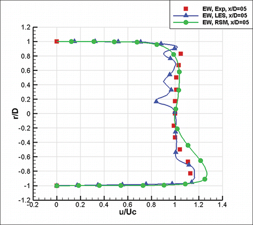
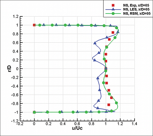
At x/D = 5, RSM once again predicted both the velocity trends and magnitudes correctly as shown in Figures 10 and 11 for E-W and N-S directions, respectively. The largest difference between experimental and CFD-RSM velocity magnitudes was approximately 8% at r/D = –0.8 in the E-W direction (Figure 10), while the error was less than 7% in the N-S direction (Figure 11). The LES predicted the velocity trends correctly although the magnitude of the velocities still exhibited relatively large errors at x/D = 5.

Fig. 10. Comparison of RSM and LES models against experimental data at x/D = 5 (E-W).

Fig. 11. Comparison of RSM and LES models against experimental data at x/D = 5 (N-S).

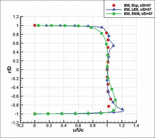
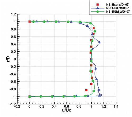
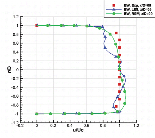
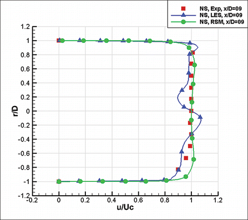
At x/D = 7, RSM predictions were accurate for both the velocity trends and magnitudes as shown in Figures 12 and 13 for E-W and N-S directions, respectively. The difference between experimental and CFD-RSM velocity magnitudes were less than 7% at r/D = –0.8 in the E-W direction (Figure 11), while the error was less than 6% in the N-S direction (Figure 12). The LES predicted both the velocity trends and magnitudes correctly, although the magnitude of the velocities still exhibited a maximum error of about 16% at x/D = 7. At x/D = 9, which is close to the second elbow, RSM predictions of both velocity trends and magnitudes were still accurate to within 6% error as shown by Figures 14 and 15. However, LES velocity trends and magnitudes started to display high error, suggesting that LES prediction accuracy was affected by the presence of the elbow. At the outlet of the elbow where x/D = 10 both, RSM and LES predicted the velocity trends and magnitudes correctly, with more accurate predictions credited to RSM (see Figure 16).

Fig. 12. Comparison of RSM and LES models against experimental data at x/D = 7 (E-W).

Fig. 13. Comparison of RSM and LES models against experimental data at x/D = 7 (N-S).

Fig. 14. Comparison of RSM and LES models against experimental data at x/D = 9 (E-W).

Fig. 15. Comparison of RSM and LES models against experimental data at x/D = 9 (N-S).

Fig. 16. Comparison of RSM and LES models against experimental data at x/D = 10 (N-S).

Conclusion

This article has presented experimental velocity profiles data and CFD predictions using RSM and LES turbulence modeling for Z-shape close-coupled five-gore elbows having nominal diameter of 305 mm (12 in) with the turning radii of the elbows fixed at r/D = 1.5. The duct length (L_int / D) separating the center-points of the elbows was systematically increased. Detailed point velocity profile measurements were performed along two perpendicular radial directions using a five-hole directional velocity probe and the results were compared to CFD predictions.

For Z-configuration, there was a velocity deficit in the elbow throat 1D downstream of the first elbow along the E-W traverse. By contrast along the E-W traverse for x/D = 1 the air had congregated in the heel of the elbow. In the N-S direction the minimum velocities at x/D = 1 were located at the center of the duct while the greatest velocities were near the north and south walls. Likewise, 1D downstream of the first elbow the minimum fluid velocity in the N-S traverse was always present at the duct centerline, further illustrating that as flow occurred around the first elbow the higher momentum fluid initially located along the centerline was pushed to the heel of the elbow, yielding a velocity deficit along the flow axis in all traverse directions.

A diminishing velocity deficit was observed up to x/D ≅ 7. However, by x/D = 9 the flow began to resemble the fully developed profile observed upstream of the first elbow both in the N-S and E-W traverse directions. At a measurement location one diameter downstream of the second elbow there was a readily apparent velocity deficit in the elbow throat, however there was virtually no corresponding increased velocity in the heel region of the elbow. It was found that although the flow downstream of the first elbow exhibited considerable swirl, for x/D ≥ 1 there was no apparent flow reversal.

RSM turbulence modeling predicted the velocity trends correctly at all x/D locations with a maximum error of 15% at x/D = 1. On the other hand, LES modeling failed to predict the trend and the magnitude of the velocities, thus LES approach is not suitable for this type of flow.

Nomenclature
A	=	= cross-sectional area of duct, m2 (ft2)
An	=	= nozzle area, m2 (ft2)
Cn	=	= nozzle discharge coefficient, dimensionless
C	=	= elbow pressure loss coefficient, dimensionless
c	=	= confidence level, dimensionless
D	=	= duct diameter, m (ft)
f	=	= friction factor, dimensionless
g	=	= gravitational constant,
L	=	= length of ductwork between specified planes, m (ft)
Lint	=	= intermediate duct length, m (ft)
N	=	= number of elements, dimensionless
PAPC	=	= pitch angle pressure coefficient, dimensionless
pv	=	= velocity pressure, Pa (in. wg)
pt	=	= total pressure, Pa (in. wg)
ps	=	= static pressure, Pa (in. wg)
v	=	= mean velocity pressure, Pa (in. wg)
Δpf	=	= duct pressure loss, Pa (in. wg)
Δps	=	= static pressure loss, Pa (in. wg)
Δpt	=	= total pressure loss, Pa (in. wg)
Q	=	= volumetric flow rate,
Re	=	= Reynolds number, dimensionless
R2	=	= coefficient of determination, dimensionless
r	=	= radius, m (ft)
S2xx	=	= squared deviation of x-data, Pa2 (in. wg2)
S2yx	=	= square of the standard error of y-data, Pa2 (in. wg2)
ta/2, N − 1	=	= t-statistic, dimensionless
V	=	= velocity,
	=	= mean air velocity,
VPC	=	= velocity pressure coefficient, dimensionless
Yn	=	= nozzle expansion factor, dimensionless

Greek symbols
α	=	= yaw angle, rad
β	=	= flow pitch angle, rad
ϵ	=	= relative surface roughness, m (ft)
ρ	=	= density,
μ	=	= dynamic viscosity,

Subscripts
E	=	= east
e	=	= exit plane
N	=	= north
r	=	= root-sum-square
S	=	= south
W	=	= west
x	=	= plane 1, 2, - - -, n, as applicable
z	=	= upstream plane

Additional information

Funding

The authors wish to thank the American Society of Heating, Refrigerating, and Air Conditioning Engineers (ASHRAE) for the financial support under research project number RP-1682.

References

- ANSYS. 2009. FLUENT 12.0. User's Manual, Ch. 4. Canonsburg, PA: ANSYS, Inc.
- ASHRAE. 2015. Duct Fitting Database Version 6.00.04. Atlanta: ASHRAE.
- Gan, G., and S.B. Riffat. 1995. K-factors for HVAC ducts: Numerical and experimental determination. Building Service Engineering Research and Technology 16(3):133–9.
- Gibbs, D.C., and S. Idem. 2012. Measurements of flat oval diverging-flow fitting loss coefficients. ASHRAE Transactions 118(1):1146–53.
- Gutovic, M., H. Lulic, and E. Sirbubalo. 2013. CFD analysis of pressure losses in flat-oval duct fittings. ASHRAE Transactions 119(2):330–40.
- Idem, S. 2003. Main loss coefficients for flat oval tees and laterals. ASHRAE Transactions 109(1):456–61.
- Idem, S., and F. Khodabakhsh. 1999. Influence of area ratio on flat oval divided flow fitting loss coefficients. HVAC&R Research 5(1):19–33.
- Kulkarni, D., J. Cui, and S. Idem. 2011. Laboratory testing of converging flow flat oval tees and laterals to determine loss coefficients. HVAC&R Research 17(5):710–25.
- Kulkarni, D., S. Khaire, and S. Idem. 2009. Measurements of flat oval elbow loss coefficients. ASHRAE Transactions 115(1):35–47.
- Liu, W., Z. Long, and Q. Chen. 2012. A procedure for predicting pressure loss coefficients of duct fittings using computational fluid dynamics. HVAC&R Research 18(6):1168–81.
- Mahank, T.A., and S.A. Mumma. 1997. Flow modeling of flat oval ductwork elbows using computational fluid dynamics. ASHRAE Transactions 103(1):172–7.
- Manning, A., J. Wilson, N. Hanlon, and T. Mikjaniec. 2013. Prediction of duct fitting losses using computational fluid dynamics. HVAC&R Research 19(4):400–11.
- Mumma, S.A., T.A. Mahank, and Y.P. Ke. 1997. Close coupled ductwork fitting pressure drop. HVAC&R Research 3(2):158–77.
- Mumma, S.A., T.A. Mahank, and Y.P. Ke. 1998. Analytical determination of duct fitting loss-coefficients. Applied Energy 61:229–47.
- Mylaram, N.K., and S. Idem. 2005. Pressure loss coefficient measurements of two close-coupled HVAC elbows. HVAC&R Research 11(1):133–46.
- Rahmeyer, J. 2002. Pressure loss coefficients for close-coupled pipe ells. ASHRAE Transactions 108(1):390–406.
- RP-551. 1991. Laboratory study to determine flow resistance of HVAC duct fittings. Final report. Atlanta, GA: ASHRAE
- RP-690. 1994. Laboratory study to determine flow resistance of oval ducts and fittings. Final report. Atlanta, GA: ASHRAE
- RP-1319. 2008. Laboratory testing of duct fittings (flat oval elbows) to determine loss coefficients. Final report. Atlanta, GA: ASHRAE
- RP-1488. 2011. Laboratory testing of flat oval fittings to determine loss coefficients. Final report. Atlanta, GA: ASHRAE
- RP-1493. 2011. CFD shootout contest—Prediction of duct fitting losses. Final report. Atlanta, GA: ASHRAE
- RP-1606. 2014. Laboratory testing of flat oval transitions to determine loss coefficients. Final report. Atlanta, GA: ASHRAE
- RP-1682. 2015. Study to identify CFD models for use in determining loss coefficients. Final report. Atlanta, GA: ASHRAE
- Sami, S., and J. Cui. 2004. Numerical study of pressure losses in close-coupled fittings. HVAC&R Research 10(9):539–52.
- Salehi, M., A.K. Sleiti, and S. Idem. 2017a. Study to identify computational fluid dynamics models for use in determining HVAC duct fitting loss coefficients. Science and Technology for the Built Environment 23(1):181–91, DOI: 10.1080/23744731.2016.1204889.
- Salehi, M., S. Idem, and A.K. Sleiti. 2017b. Experimental determination and CFD predictions of pressure loss in close-coupled elbows. Journal of Science and Technology for the Built Environment Accepted STBE-00204-2016. Accepted author version posted online January 3, 2017. http://dx.doi.org/10.1080/23744731.2016.1268904.
- Sleiti, A.K., J. Zhai, and S. Idem. 2013. Computational fluid dynamics to predict duct fitting losses: Challenges and opportunities. HVAC&R Research 19(1). http://www.tandfonline.com/doi/abs/10.1080/10789669.2012.716341.
- Townsend, B., F. Khodabakhsh, and S. Idem. 1994. Equivalent round diameter of spiral flat oval ducts. ASHRAE Transactions 100(2):389–95.
- Townsend, B., F. Khodabakhsh, and S. Idem. 1996a. Loss coefficient measurements in divided-flow flat oval fittings. ASHRAE Transactions 102(2):151–8.
- Townsend, B., F. Khodabakhsh, and S. Idem.1996b. Loss coefficient measurements for flat oval elbows and transitions. ASHRAE Transactions 102(2):159–69.
- Treaster, A.L., and Yocum, A.M. 1979. The calibration and application of five-hole probes. ISA Transactions 18:23–34