Assessment and improvement of the 2019 ASHRAE handbook model for exhaust-to-intake dilution calculations for rooftop exhaust systems (ASHRAE 1823-RP)

Abstract

The HVAC Applications volume of the 2019 ASHRAE Handbook: Chapter 46 gives multiple procedures for sizing building exhaust stacks and fans. The most complex of these procedures directly calculates dilution at a receptor of interest using plume theory and several empirical constants. There is suggestion in the literature that this model leads to overly conservative dilution predictions in some cases. The purpose of this work is to determine whether the ASHRAE model can be improved to give more accurate dilution predictions. First, the predictions of the existing equation are evaluated against several existing wind tunnel and full-scale studies and their shortcomings noted. The results show that the 2019 model under-predicts observed dilution mainly in two cases: near the stack and when the plume is within the assumed recirculation region. The assumptions for initial plume spread, height of recirculation zone region, plume spread and plume trajectory were varied parametrically to identify a better model. This optimized model can increase dilution predictions by factors between 2 and 500, while bounding measured data in all cases analyzed. This can reduce the required momentum ratio by 20–70%, leading to much more efficient fan sizing and operation.

Introduction and problem statement

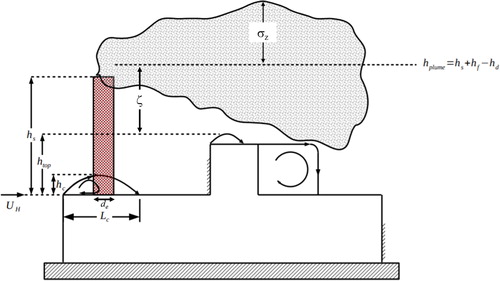
The 2019 ASHRAE Handbook: HVAC Applications volume provides a model in Chapter 46 that predicts dilution from rooftop exhaust stacks at receptors on building roofs and elsewhere, referred to here forward as simply “the model”. This model is explained in detail in Appendix A of the current work, and briefly outlined presently, with variables called out in Figure 1. The model works by first calculating plume height (h_plume) at each distance from the exhaust, which is the plume rise from the stack (h_r) added to the stack height (h_s) minus the plume downwash (h_d). This plume height is then modified to account for the presence of rooftop structures and the building recirculation zone (the vertical height of which is referred to as h_c), via the h_top parameter which is described in detail below. This modified height is used in conjunction with a prediction of plume spread in the vertical and lateral directions to predict a dilution between the exhaust and any receptor of interest.

Fig. 1 Flow recirculation zones and other geometrical exhaust parameters (ASHRAE 2019-Modified).

Several shortcomings in this model have been identified in the literature. Hajra, Stathopoulos, and Bahloul (2011) shows that the ASHRAE model is overly conservative in many cases. Gupta, Stathopoulos, and Saathoff (2012) also claim that the model predicts dilution conservatively, especially when an obstacle exists on the roof. Gupta, Stathopoulos, and Saathoff (2012) mention that the ASHRAE model is more accurate as the distance from the stack is increased.

The plume trajectory may be one source of error. Virtually all validation of the model was done by measurements or photographs of the plume far from the stack (Briggs 1973). The region of interest in building design is often the very-near field and to the authors’ knowledge the plume trajectory has not been validated in this region. This is investigated further in the current work.

Other variables that play an important role in predicting plume dilution include the initial source size, σ_o, and the vertical and lateral plume spreads, σ_y and σ_z. ASHRAE RP 897 (Wilson et al. 1998) suggested the following equation be used for calculating the initial source size. (1) $$\begin{array}{c}{\sigma }_0={\left(\frac{M}{8}+\frac{{\beta }_{\mathit{eff}}^2}{2}{\left(\frac{\Delta h}{d}\right)}^2+{0.5}^2\right)}^{0.5}d \end{array}$$(1) (2) $$\begin{array}{c}{\beta }_{\mathit{eff}}=\frac{1+0.015M^2}{1+0.04M^2} \end{array}$$(2) where M is the exhaust momentum ratio [-], $\Delta h$ is the final momentum rise height = 3Md [m,ft], and d is the stack diameter [m, ft].

In the 2019 Handbook, σ_o is set to 35% of the exhaust diameter, d_e, which is based on the conservative assumption of a momentum ratio equal to 1 and a simplified version of Equation 2(2) $$\begin{array}{c}{\beta }_{\mathit{eff}}=\frac{1+0.015M^2}{1+0.04M^2} \end{array}$$(2) (Wilson 2019). In the experiments of ASHRAE RP 897, Equation 1(1) $$\begin{array}{c}{\sigma }_0={\left(\frac{M}{8}+\frac{{\beta }_{\mathit{eff}}^2}{2}{\left(\frac{\Delta h}{d}\right)}^2+{0.5}^2\right)}^{0.5}d \end{array}$$(1) predicts σ_o between 1d_e and 2.5d_e for momentum ratio of 1. For the studies analyzed in this work, Equation 1(1) $$\begin{array}{c}{\sigma }_0={\left(\frac{M}{8}+\frac{{\beta }_{\mathit{eff}}^2}{2}{\left(\frac{\Delta h}{d}\right)}^2+{0.5}^2\right)}^{0.5}d \end{array}$$(1) predicts between 1d_e and 3d_e for momentum ratios less than 1, between 3d_e and 5d_e for momentum ratios between 1 and 2, and between 6d_e and 15d_e for momentum ratios up to 5. Anecdotal conversations between the authors and practitioners confirmed that it is often necessary to set this value near one in order to predict dilution values that match wind tunnel results.

Plume spread is calculated by first calculating the lateral and vertical components of turbulence intensity, i_y and i_z, by multiplying the longitudinal component i_x by empirical constants. Early in the literature turbulence was assumed to be equal in x, y and z directions. Scrase (1930) measured the three components at two different heights (1.5 and 19 meters; [4.9 and 62 ft]). He found the ratio of y and z components to x were 1.16 and 0.75, respectively, at a height of 1.5 meters [4.9 ft], and 0.73 and 0.56 at 19 meters [2.4, 1.8, 62 ft]. The 2019 ASHRAE Handbook procedure agrees with the measurements made at a height of 19 meters [62 ft]. Scrase (1930) also mentioned that at heights greater than 60 meters [200 ft] the velocity components can be assumed to be equal. Teunissen (1970) measured turbulence intensity variation with height over a flat terrain. His experiments show that although the turbulence intensities decrease with height, the ratio of lateral and vertical to horizontal turbulence intensities are constant with height.

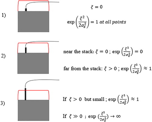
Another source of error is likely in the concept of h_top, which is the highest of either the receptor of interest, the top of the building recirculation zone, or the tallest of the “active obstacles”. This variable is introduced via another variable, ζ, which is the difference between the exhaust plume height and h_top. The relationship between ζ and h_top leads to one of the following scenarios, depicted in Figure A1 in Appendix A:

1. The predicted plume height, h_plume, is less than h_top at all distances from the stack. In this case, ζ becomes zero at all distances and the minimum dilution is predicted using only the non-exponential term in the model. This leads to a counterintuitive situation in which increasing exhaust velocity decreases prediction of dilution.

2. Predicted h_plume is less than h_top near the stack, and greater far from the stack. In this case since the difference between h_plume and h_top is small, the exponential term is around one and near-constant dilution is predicted at all distances from the stack.

3. h_plume is greater than h_top at all distances from the stack. In this case ζ is always non-zero and the exponential term is effective. In this case the exponential term may approach infinity near the stack, and as a result the model predicts a very high dilution near the stack.

Since many have measured a recirculation zone above building roofs, the inclusion of h_top was an intuitive and understandable one. However, to the authors’ knowledge data-driven optimization of the effective height of this region or rigorous justification of its inclusion for exhaust plume modeling has not been performed, and a few shortcomings that motivate the current work are mentioned above.

In light of these possible shortcomings in the current model, this investigation pursues three objectives:

1. Assess the existing model and compare it with published data to identify situations in which the model can be improved.

2. Identify model parameters that can be improved and which lack physical or empirical justification.

3. Optimize the values of these parameters and make any other modifications necessary to improve model predictions while ensuring the model does not overpredict dilution in any published cases.

Methodology

In order to evaluate the existing model, published wind tunnel and full-scale dilution data were first assembled in a database and reviewed. The database included data from the following sources:

1) Hajra, Stathopoulos, and Bahloul (2011)

General details of this dataset are as follows:

• Two building heights of 15 and 30 m [49 and 98 ft], referred to as low rise and high rise building, respectively.

• 4 different building configurations with 3 different stack heights [1, 3, 5 m (3.28 ft, 9.84 ft, 16.4 ft)] and 3 momentum ratios: 1, 2, 3.

For this evaluation only data from the configurations where no neighboring buildings existed were used. Experimental data from the case with 5 m [16 ft] stack height and momentum ratio of 2 was not reported in the article.

2) Gupta, Stathopoulos, and Saathoff (2012)

General details of this dataset are as follows:

• 5 different exhaust momentum ratios, and 4 different stack heights were tested:

• Stack heights h_s (m): 1, 3, 5, 7 [3.3, 10, 16, 23 ft]

• Exhaust momentum ratios (M = V_e/U_H): 1, 2, 3, 4, 5

• Two building heights of 15 [49ft] and 60 m [197 ft], called low rise and high rise building respectively.

In this evaluation only experimental data from the tests where no rooftop structure existed on the roof were used. Dilution values from the experiments with stack heights of 3 m [10 ft] were reported in the article.

3) ASHRAE Research Project 805: Petersen, Carter, and Ratcliff (1997)

General details of this dataset are as follows:

• 3 different volumetric flow rates and 6 different stack heights were tested.

• Stack heights (hs): 0, 1, 3, 5, 7, 12 ft (0, 0.3, 0.9, 1.5, 2.1, 3.7 m)

• Wind azimuths: 0, 45 and 90 degrees

This dataset included tests with screens on the roof. In this evaluation only data from the experiments without any screens on the roof were used.

4) Schulman and Scire (1991)

General details of this dataset are as follows:

• 4 different exhaust momentum ratios, 4 different stack heights, and 2 different angles were tested.

• Stack heights (hs): 0, 1.5, 4.5, 7.5 m [0, 5, 15, 25 ft]

• Exhaust momentum ratios (M = V_e/U_H): 0.75, 1.5, 3, 5

• Wind azimuths: 0 and 45 degrees

In this dataset, some data points were from the receptors located on a sidewall. In this evaluation, those data points have been excluded and the focus was on the data points from receptors located on the rooftop only, but at the end the sidewall data points were also checked with our findings.

5) Wilson and Chui (1994)

General details of this dataset are as follows:

• 11 building configurations with 6 different exhaust momentum ratios were tested.

• Stack heights (hs): 0, 2.44, 3.66 (m) [0, 8, 12 ft]

• Exhaust momentum ratios (M = V_e/U_H(avg)): ranged from 0.19 to 2.86

In this dataset all models had round, vertically directed exhaust jets of zero stack height.

6) Wilson and Lamb (1994)

General details of this dataset are as follows:

• Tests were full scale.

• 11 different exhaust momentum ratios and 11 model building configurations were tested.

• Stack heights (hs): 0, 2.44, 3.66 m [0, 8, 12 ft]

• Exhaust momentum ratios (M = Ve/U_H(avg)): ranged from 1.23 to 8.48

This dataset includes data from a field study done on a group of building located on a university campus, using 44 receptors located both on the roof and on the ground.

For each data point the dilution values were calculated with the 2019 ASHRAE procedure and the predicted and observed values of dilution were plotted to compare. In order to facilitate comparison, R is defined as the ratio of observed to predicted dilution: (3) $$\begin{array}{c}R=\frac{D_{\mathit{Observed}}}{D_{\mathit{Predicted}}}\end{array}$$(3)

Using this definition: $$\mathrm{if}\mathrm{ }R<1\mathrm{ }\to \text{ASHRAE model is failing}$$ $$\mathrm{if}\mathrm{ }R>1\mathrm{ }\to \text{ASHRAE model is bounding the data}$$ $$\mathrm{if}\mathrm{ }R\gg 1\mathrm{ }\to \text{ASHRAE model is too conservative}$$

The ultimate purpose of this work is to define a model that bounds the data without being overly conservative, or result in R that approaches 1.

Several methods for improving the current model were attempted, guided by previous literature and assessment of the shortcomings of the current model. One of these involved modification of the assumption for h_top, which was suggested in previous literature and justified in this work. The other three involved modifying assumptions for plume geometry near the stack, which was suggested by the consistently overly conservative predictions near the stack calculated in this work. They are as follows:

1. Identification of an optimal height for h_top by introducing parameter a in the current model and identifying its optimal value: (4) $$\begin{array}{c}\zeta =h_{\mathit{plume}\mathrm{ }}- \alpha h_{\mathit{top}}\end{array}$$(4)

2. Identification of optimal value for initial source size by introducing parameter $\gamma$ (5) $$\begin{array}{c}\gamma =\frac{{\sigma }_0}{d_e}\end{array}$$(5)

   This convention allows for a simple formulation for initial source size, but one that is optimized to give the least conservative value.

3. Identification of an optimal model of plume spread in the near field, by including a term, $i_{\mathit{self}},\mathrm{ }$ that acts as turbulence within the plume immediately leaving the stack and a gradual transition a few stack diameters away to the current model, enabled by the parameter p in Equations 6(6) $$i_y=0.75 i_x+\left(i_{\mathit{self}}-0.75\mathrm{ }{i}_x\right)\frac{p}{\left(\frac{x}{d_e}\right)+p}$$(6) and 7(7) $$i_z=0.5 i_x+\left(i_{\mathit{self}}-0.5\mathrm{ }{i}_x\right)\frac{p}{\left(\frac{x}{d_e}\right)+p}$$(7) .

   (6) $$i_y=0.75 i_x+\left(i_{\mathit{self}}-0.75\mathrm{ }{i}_x\right)\frac{p}{\left(\frac{x}{d_e}\right)+p}$$(6) (7) $$i_z=0.5 i_x+\left(i_{\mathit{self}}-0.5\mathrm{ }{i}_x\right)\frac{p}{\left(\frac{x}{d_e}\right)+p}$$(7)

   Because the assumptions in the current model for vertical and lateral plume spread in the far field are based on measured values of turbulence intensity in these directions, these variables are not modified in the course of this work. The effect of the term i_self is likely the summation of several mechanisms including expansion of the jet immediately upon leaving the exhaust.

4. Identification of optimal assumption for plume trajectory in the near-field through the introduction of the parameter $\delta$ in Equation 8(8) $$\begin{array}{c}{h}_{\mathit{plum}{e}_{\mathit{modified}}\mathrm{ }}=h_{\mathit{plume}}+\delta \times (h_f+h_s-h_{\mathit{plume}})\end{array}$$(8) in which h_s is the stack height and h_f is the final plume rise from the stack (Formulation to calculate the final plume rise is from the ASHRAE handbook). This allows for an increase in plume height near the stack, which seemed to be justified after a review of the performance of the current model in this region. (8) $$\begin{array}{c}{h}_{\mathit{plum}{e}_{\mathit{modified}}\mathrm{ }}=h_{\mathit{plume}}+\delta \times (h_f+h_s-h_{\mathit{plume}})\end{array}$$(8)

   In order to identify values for these parameters that resulted in a model that bounded measured data as conservatively as possible the objective function F was defined as (9) $$\begin{array}{c}F (\alpha ,\gamma , i_{\mathit{self}},p,\delta )=\sqrt{\sum {\left(R-1\right)}^2}\end{array}$$(9)

A MATLab program was developed to minimize this F by changing the variables $\alpha ,\gamma ,\mathrm{ }{i}_{\mathit{self}},p,\text{ and }\delta .$ (0 < α`1, 0 < γ`5, 0`$\mathrm{ }{i}_{\mathit{self}}$<1, 0<p < 5, 0 < δ < 20). For each dataset, all data points (observed dilutions) were added into MATLab as a table. For each observed dilution all parameters needed to calculate the minimum dilution were also added, including the distance from the stack at which that dilution was observed (x), the plume rise (h_plume), and etc. The program then systematically changes the variables and checks the resulting value of R. If the value of R is less than 1, the code discards that set of parameters and continues to check the rest of the parameters systematically. Finally, it reports the set of parameters at which F is a minimum.

When optimizing the parameters, the number of failings (points in which D_predicted>D_observed) were limited to the number of failings observed before optimization. In other words, the parameters were optimized in such a manner that the number of failing points with the optimized parameters was less than or equal to the number of failing points in the existing model.

In performing the optimization, it became clear that a cutoff value for the exponential term of the model needed to be added to prevent it from approaching infinity close to the stack. This cutoff value is 1096 (exponential of 7). This cutoff value was implemented in the older versions of the ASHRAE model to avoid the exponential term approaching infinity close to the stack. The authors are unaware of why it was discarded in the latest version.

Data from Gupta, Stathopoulos, and Saathoff (2012), Hajra, Stathopoulos, and Bahloul (2011), Schulman and Scire (1991), and Petersen, Carter, and Ratcliff (1997) were used to identify optimal values of the parameters in question. Once these values were identified, the new model was validated against the large data sets of Wilson and Lamb (1994) and Wilson and Chui (1994), and tested for its performance on the data in Petersen, Carter, and Ratcliff (1997) which was taken in setups that contained screens and from Schulman and Scire (1991) taken on sidewalls.

Results

Existing model evaluation

In the following section a comparison of the dilution predicted by the ASHRAE model and that measured in the wind tunnel experiments is presented. For each configuration, the predicted dilution curve is calculated using that configuration’s stack height, building height and momentum ratio and plotted as a solid line. Measured data is plotted as points and color-coded according to input conditions.

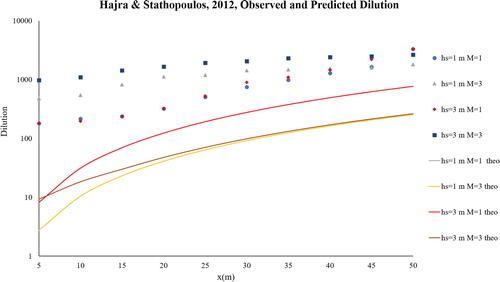
1) Hajra, Stathopoulos, and Bahloul (2011)

There are two recognizable trends shown in this figure:

1. The difference between the predicted and observed dilution is more significant near the stack (approaching two orders of magnitude) and decreases farther from the stack.

2. The difference between the predicted and observed dilution is greater for higher stacks and greater momentum ratios (higher plume rise).

In other words, Figure 2 shows that the model under-predicts the dilution (predicts more conservatively) near the stack and for higher plume rises.

Fig. 2 Observed and predicted dilutions for Hajra, Stathopoulos, and Bahloul (2011) (Points are measured observations and curves are model predictions).

2) Gupta, Stathopoulos, and Saathoff (2012)

In this dataset, the effect of building height on dilution predictions is recognizable. The yellow curve in Figure 3 shows predicted dilution for the low-rise building with a stack height of 3 m [10 ft] and momentum ratio of 5. At the other extreme, the black curve shows predicted dilution for the same stack height and momentum ratio, but for the high-rise building. The momentum ratio of 5 is the highest momentum ratio in these experiments so these tests have the highest plume rise (from the roof level) compared to others. As shown in the figure, the model under-predicts dilution for the high-rise building while over-predicting it in the low-rise building.

Fig. 3 Observed and predicted dilutions from Gupta, Stathopoulos, and Saathoff (2012) (Points are measured observations and curves are model predictions).

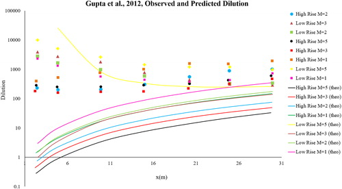
There are two ways to explain the reason for this phenomenon. From a mathematical point of view, the height of the building recirculation zone (h_top) is higher in the high-rise building compared to the low-rise building, since it is a function of building dimensions. Also, for a high momentum ratio, the plume rise (h_plume) is high. Minimum dilution, according to ASHRAE 2015, is a function of the vertical separation (ζ), which is the difference between h_plume and h_top. For the same stack height and momentum ratio, h_plume has the same value, so in the low-rise building where h_top is small, ζ becomes high and the ASHRAE model predicts high values of dilution, while in the high-rise building it does the opposite.

Another factor that may come into play is the vertical atmospheric turbulence intensity gradient. Since turbulence intensities decrease as the height of the building increases, turbulence intensities are less for the high-rise building. As a result, for the same plume rise lower dilutions are achieved compared to the low-rise building. In other words, in the low-rise building the plume is more diluted compared to the high-rise building due to higher atmospheric turbulence near the ground.

3) ASHRAE Research Project 805, Petersen, Carter, and Ratcliff (1997)

Figure 4 shows two extreme cases from this article¹, one with the least momentum ratio (M = 0.3) and the other with the greatest momentum ratio (M = 3.5), both from the tests with zero-degree wind direction.

Fig. 4 Observed and predicted dilutions from Petersen, Carter, and Ratcliff (1997) (Points are measured observations and curves are model predictions).

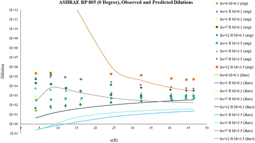
Figure 4 shows that for the least momentum ratio (M = 0.3), no matter what the stack height is, the model is predicting the same values (prediction curves collapse into one). This is because in these cases the plume rise (h_plume) is below the height of the recirculation zone (h_top); thus, the vertical separation (ζ) equals zero and the minimum dilution is calculated by the non-exponential term of the ASHRAE model, which is a function of the momentum ratio and not the stack height, a shortcoming of the current model referred to previously.

For the greater momentum ratio (M = 3.5), it is shown that for stack heights of 1 and 3 ft, the model is under-predicting the dilution. In these two cases the value of h_plume is less than or very close to the value of h_top, so that the exponential term of the ASHRAE model is approximately 1, and the minimum dilution is mainly predicted by the non-exponential term of the model. As the stack height increases (h_s=7 ft [2 m]) the exponential term of the model becomes more effective, changing the shape of the curve. For this stack height (h_s=7 ft) the shape of the curve (predicted dilution) exactly follows the pattern of experimental data points, but as the stack height increases from 7 to 12 ft [2 to 3.6 m], the model suddenly approaches infinity near the stack. As shown in Figure 4, the model is over predicting the dilution near the stack, which is mathematically due to the large difference between the value of h_plume and h_top which leads to a high value of ζ and thus a large exponential term. It is also worth mentioning that in this case (h_s=12 ft [3.6 m]), the predicted values for dilution near the stack are far beyond the values that can be measured (greater than 10⁷). One modification this suggests is enforcing an upper bound on the dilution predictions; one possible value is 10⁷ which to our knowledge is the greatest value measured in the literature. Another option would be adding a cutoff value on the exponential term, as explained before.

4) Schulman and Scire (1991)

Figure 4 shows two extreme cases of this article², one with the lowest stack (h_s=0) and the other with the highest stack (h_s=7.5 m [25 ft]), both from the tests with zero-degree wind direction. Figure 4, shows that for a stack height of zero, both the predicted and observed dilution increase as the distance from the stack is increased for lower momentum ratios (M = 0.75, 1.5), while for the greater momentum ratios (M = 3, 5) the predictions increase with x, while the observations decrease. Also, for a stack height of zero, the model predicts lower dilutions for greater momentum ratios (M = 3, 5 compared to M = 0.75, 1.5), while the experiments show greater dilutions for greater momentum ratios. The reason is that in these cases the plume rise is so small that the difference between h_top and h_plume becomes small and the exponential term is around 1. Thus, the minimum dilution is mainly calculated by the non-exponential term, which is inversely related to the momentum ratio, so for lesser momentum ratios the model predicts greater dilution.

In reality, greater momentum ratios produce greater dilutions. In fact, fan speed is one of only a few design variables a designer might change in order to improve the performance of the exhaust, and in this case increasing fan speed decreases predicted dilution. This is a major shortcoming of the model and shows that the exponential term of the model should be effective to make the prediction closer to reality and this only happens when the vertical separation (ζ) increases which requires h_top to be lower (Figure 5).

Fig. 5 Observed and predicted dilutions from Schulman and Scire (1991) (Points are measured observations and curves are model predictions).

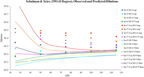
For the stack height of 7.5 m [25 ft], when the momentum ratios are small (M = 0.75, 1.5), the prediction curves are conservatively bounding the data points. While, for greater momentum ratios (M = 3, 5), the model predicts unrealistically large values near the stack. As shown in Figure 4, the model over-predicts dilution near the stack, which is mathematically due to the large difference between the value of h_plume and h_top which leads to a high value of ζ and large exponential term. Again it is also worth mentioning that in these cases (M = 3, 5), the predicted values for dilution near the stack are far beyond those that can be measured (greater than 10⁷).

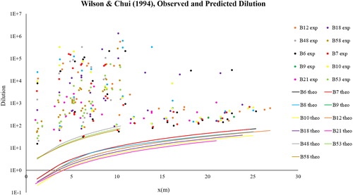
5) Wilson and Chui (1994)

As shown in Figure 6, in this dataset all experimental data points are bounded by the prediction curves. This is due to the fact that since the stack height was zero (plume always within recirculation zone or less than h_top), the exponential term of the ASHRAE model was approximately 1 for all cases, and the minimum dilution was mainly calculated by the non-exponential term of the model. Based on our investigation and Gupta, Stathopoulos, and Saathoff (2012), it is clear that when only the non-exponential term is active, the ASHRAE model tends to predict conservatively.

Fig. 6 Observed and predicted dilutions from Wilson and Chui (1994) (Points are measured observations and curves are model predictions).

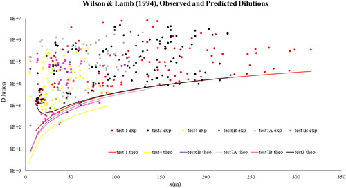
6) Wilson and Lamb (1994)

This dataset was not directly used to develop the existing ASHRAE model according to ASHRAE RP 1635, in which an average of all tests was used to compare the new suggested equation and experimental data. Our investigation showed that when all experimental points are plotted separately, the handbook model fails to bound some data points (Figure 7).

Fig. 7 Observed and predicted dilutions from Wilson and Lamb (1994) (Points are measured observations and curves are model predictions).

In summary, the important takeaways from our investigation into the wind tunnel data are as follows:

• The 2019 ASHRAE model under-predicts dilution (conservative) closer to the stack. This may be due to inaccurate prediction of the plume trajectory, inaccurate prediction of the plume spread in the near field, or a combination of the two.

• The predictions near the stack approach infinity (>10⁷) in some cases.

• Building dimensions affect the predictions significantly, since h_top is calculated based on the building dimensions.

• There are cases in which, since the exponential term is zero (h_plume<h_top), and the non-exponential term of the model is inversely related to the momentum ratio, for greater momentum ratios the existing model predicts less dilution, which is physically unjustifiable.

Optimization

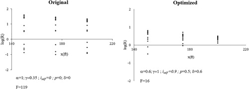
Using data from Gupta, Stathopoulos, and Saathoff (2012), Hajra, Stathopoulos, and Bahloul (2011), Schulman and Scire (1991), and Petersen, Carter, and Ratcliff (1997), optimal values of the parameters in question were identified. Table 1 shows the progressive improvement of the model through addition and optimization of each variable. Table 2 shows the final optimization, the values of the parameters identified, and the physical meaning of each variable.

Table 1 Progressive improvement of model through addition of variables and effect on objective function.

Case	α	γ	iself	P	δ	Number of Failings	F
Original	1	0.35	0	0	0	10	439,477
Optimized γ	1	1.7	0	0	0	10	90,750 (21%)
Optimized α & γ	0.6	1	0	0	0	10	21,062 (4.8%)
Optimized α, γ, iself , p, and δ	0.6	1	0.9	0.5	0.6	9	7,987 (1.8%)

Table 2 Physical meaning of defined parameters.

Parameter	Previous value	Optimal value	Physical meaning
α	1	0.6	Active portion of recirculation zone can be assumed to 40% below height of recirculation zone, avoiding difficulties cited above
γ	0.35	1	Initial source size can be assumed to be equal to the width of the exhaust stack
iself	0	0.9	Plume spread immediately leaving stack behaves as if there were initial turbulence intensity of 90% in lateral and vertical directions. This is likely due to several mechanisms.
p	0	0.5	Parameter defining the distance from the stack at which plume spread is dominated by atmospheric turbulence rather than self-induced turbulence in the plume.
δ	0	0.6	Plume trajectory in near-field is assumed to be 60% between previously assumed plume trajectory and final plume rise.

According to Table 1 and Table 2, by simply reducing h_top by 40% and increasing the initial source size to the stack diameter, a decrease from 439,477 to 21,062 in the objective function F results. Or to put it another way, the average dilution prediction analyzed became less conservative by approximately half an order of magnitude. If more accuracy in predictions is desired, the following modified equations for calculating turbulence intensities and plume height can be included:

(10) $$i_y=0.75 i_x+\left(0.9-0.75\mathrm{ }{i}_x\right)\frac{0.5}{0.5+\left(\frac{x}{d_e}\right)}$$(10)

(11) $$i_z=0.5 i_x+\left(0.9-0.5\mathrm{ }{i}_x\right)\frac{0.5}{0.5+\left(\frac{x}{d_e}\right)}$$(11)

(12) $$\begin{array}{c}{h}_{\mathit{plum}{e}_{\mathit{modified}}\mathrm{ }}=h_{\mathit{plume}}+0.6\times (h_f+h_s-h_{\mathit{plume}})\end{array}$$(12)

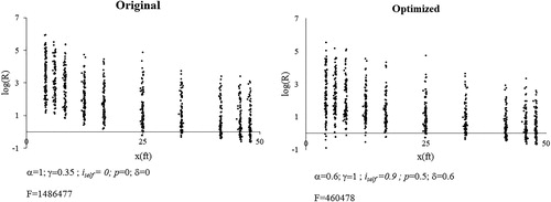
Equations 10 and 11 assume that the exhaust plume immediately leaving the stack spreads rapidly, due to turbulence within the plume, expansion upon leaving the stack, or some other mechanism. Equation 12(12) $$\begin{array}{c}{h}_{\mathit{plum}{e}_{\mathit{modified}}\mathrm{ }}=h_{\mathit{plume}}+0.6\times (h_f+h_s-h_{\mathit{plume}})\end{array}$$(12) modifies the assumption for plume trajectory in the near-stack region upward by 60% of the distance between the previously assumed trajectory and the final plume rise. These additions result in a decrease in the objective function F from 439,477 to 7,840. This can reduce the required momentum ratio by 20-70%, leading to much more efficient fan sizing and operation. This improvement in the model also alleviated several of the issues identified in the evaluation of the previous model, including reducing the influence of h_top and removing the poor performance near the stack, as shown in Figure B5 in Appendix B.

Once these values were identified, the new model was validated against the large data sets of Wilson and Lamb (1994) and Wilson and Chui (1994), and tested for its performance on the data in Petersen, Carter, and Ratcliff (1997) which was taken in setups that contained screens and from Schulman and Scire (1991) taken on sidewalls.

The results showed that the improvement of the new model with Wilson and Chui (1994) and Wilson and Lamb (1994) data sets is significant although not as profound as the improvement on the other data sets. The new model did not add any failing points (points where R < 1), and thus the new model can also be used to predict these data sets.

The new model was also checked to test its performance on tests from the receptors on the side wall (hidden intakes) from Schulman and Scire (1991). Results showed that the original model fails to bound the data points at farther distances from the stack, while with the modifications made to the model all experimental data-points are bounded by the predicted values, which is an important improvement.

The new model was also checked on tests with screens from ASHRAE RP 805 for which the original model was overly conservative near the stack and failed to bound the observations at farther distances. The results showed that for this database the modified version of the model predicts the dilution more accurately near the stack (less conservative), but the problem of having failings at farther distances still exists. The results are shown in Table 3, and the graphs of original and optimized cases can be found in Appendix B. The improvement in predictions was not as stark as with the data sets analyzed above. This is because many of these points are well off of the plume axis and for this reason large dilution was measured. It was not possible to distinguish which receptors were along the plume axis in the existing publications.

Table 3 Optimized values checked on other data sets results.

Case	α	γ	iself	p	δ	F (original)	F (optimized)	Number of failings (original)	Number of failings (optimized)
Wilson and Lamb 1994	0.6	1	0	0	0	155794	122313	9	14
Wilson and Chui 1994	0.6	1	0	0	0	301049	181162	0	0
RP 805 (tests with screens)	0.6	1	0	0	0	1486477	647931	60	60
Schulman and Scire 1991 (Hidden intakes)	0.6	1	0	0	0	119	76	11	21
Wilson and Lamb 1994	0.6	1	0.9	0.5	0.6	155794	45902	9	4
Wilson and Chui 1994	0.6	1	0.9	0.5	0.6	301049	122378	0	0
RP 805 (tests with screens)	0.6	1	0.9	0.5	0.6	1486477	460478	60	60
Schulman and Scire 1991 (Hidden intakes)	0.6	1	0.9	0.5	0.6	119	16	11	3

Conclusions and recommendations

In this project the performance of ASHRAE 2019 models for calculating the minimum dilution of the exhaust from rooftop exhaust stacks were evaluated and a few of the model’s parameters were optimized. The following summarizes the main conclusions of this study:

1. The 2019 ASHRAE Handbook model for rooftop dilution under-predicts dilution generally in two cases; first, at locations near the stack and second, in cases where the plume does not rise beyond the assumed height of the building recirculation zone.

2. Both of these problems seem to be at least partially attributable to the concept of h_top, and the near-field discrepancies are also likely due to an inaccurate description of the plume near the stack.

3. If the assumed height of h_top is reduced by 40% and the initial source size increased to be equal to the exhaust stack diameter, the conservativeness of the model is reduced by a factor of approximately 14 in the datasets analyzed herein.

5. If more complexity and more accuracy is desired, decreasing h_top by 40% from the 2019 model, increasing source size to be equal to the exhaust diameter, and augmenting the description of the near-stack plume trajectory and spread according to Equations 10(10) $$i_y=0.75 i_x+\left(0.9-0.75\mathrm{ }{i}_x\right)\frac{0.5}{0.5+\left(\frac{x}{d_e}\right)}$$(10) , 11(11) $$i_z=0.5 i_x+\left(0.9-0.5\mathrm{ }{i}_x\right)\frac{0.5}{0.5+\left(\frac{x}{d_e}\right)}$$(11) and 12(12) $$\begin{array}{c}{h}_{\mathit{plum}{e}_{\mathit{modified}}\mathrm{ }}=h_{\mathit{plume}}+0.6\times (h_f+h_s-h_{\mathit{plume}})\end{array}$$(12) will reduce the conservativeness of the model by an additional factor of 2 for the datasets analyzed herein. These measures together can reduce the required momentum ratio by 20-70%, leading to much more efficient fan sizing and operation.

6. The current model predicts dilutions of >10⁷ near the stack because of the exponential part of the model approaching infinity at small distances. To solve this problem a cutoff value of 1096 (exponential of 7) is suggested. This cutoff value was implemented in older versions of the ASHRAE model to avoid the exponential term approaching infinity close to the stack.

Fig. A1 Relationship between htop and hplume for three different scenarios.

Acknowledgments

Funding for this project was provided by ASHRAE RP-1823 as a cooperative agreement between the ASHRAE and The Ohio State University. The authors would like to thank members of the Project Monitoring Subcommittee (Brian Rock, Steve Taylor, and Iain Walker) and members of ASHRAE TC4.3 for their input. We would also like to thank Dr. David J. Wilson for briefly coming out of retirement to answer questions about the history of the ASHRAE Handbook Model, and John Carter of CPP Wind Engineers and Air Quality Consultants for insight into performance of the model in practice.

Notes

1 These two cases are two extreme samples of all cases extracted that are shown here for easier comparison. For the next steps of this project all cases where considered.

2 These two cases are two extreme samples of all cases extracted that are shown here for easier comparison. For the next steps of this project all cases were considered.

Appendix A. ASHRAE minimum dilution model

According to the 2019 ASHRAE Handbook: HVAC Applications: Chapter 46, the dilution at any receptor of interest can be predicted using a model that assumes a Gaussian profile for the plume issuing from an exhaust stack. To do this, roof-level dilution, D_r, is first defined as (A1) $$\begin{array}{c}{D}_r=\frac{C_e}{C_r}\end{array}$$(A1) where C_e is the concentration of the contaminants at the stack exit and C_r is the maximum concentration on centerline of the plume.

The plume spread (σ_y and σ_z) is then calculated using the following equations from Cimorelli et al. (2005). (A2) $$\begin{array}{c}{\sigma }_y={\left(i_y^2{x}^2+{\sigma }_o^2\right)}^{\frac{1}{2}}\end{array}$$(A2) (A3) $$\begin{array}{c}{\sigma }_z={\left(i_z^2{x}^2+{\sigma }_o^2\right)}^{\frac{1}{2}}\end{array}$$(A3) where i_y is turbulence intensity in y direction,i_z is turbulence intensity in z direction and x is the distance from the stack,σ_o is defined as a function of stack diameter (σ_o =0.35d_e).

Turbulence intensities (i_x, i_y and i_z) are calculated from the following equations: (A4) $$\begin{array}{c}{i}_y=0.75i_x ; i_z=0.5i_x\end{array}$$(A4) (A5) $$\begin{array}{c}{i}_x=\frac{n \ln \left(\frac{90.4}{z_o}\right)}{\ln \left(\frac{H}{z_o}\right)}\end{array}$$(A5) (A6) $$\begin{array}{c}n=0.19+0.096 {\log }_{10}^{z_o}+0.016{\left({\log }_{10}^{z_o}\right)}^2\end{array}$$(A6)

Finally, dilution is calculated using the following equation (A7) $$\begin{array}{c}Dr\left(x\right)=\frac{4U_H{\sigma }_y{\sigma }_z}{V_e{d}_e^2}\exp \left(\frac{{\varsigma }^2}{2{\sigma }_z^2}\right)\end{array}$$(A7)

In order to consider the effect of any rooftop structures, intakes and wind recirculation zones, the vertical separation, ζ is defined as (A8) $$\begin{array}{c}\zeta =h_{\mathit{plume}}-h_{\mathit{top}}\\ =0\mathit{\text{ if }}{h}_{\mathit{plume}}< h_{\mathit{top}}\end{array}$$(A8)

The value of h_top is defined as the tallest height of all rooftop structures and recirculation zones (H_c), which is calculated as follows (A9) $$\begin{array}{c}{H}_c=0.22R\end{array}$$(A9) (A10) $$\begin{array}{c}R=B_s^{0.67}{B}_L^{0.33}\end{array}$$(A10) where B_L is the larger upwind dimension of the building or rooftop structure and B_S is the smaller.

Figure A1 shows the relationship between $h_{\mathit{plume}} \mathrm{and} h_{\mathit{top}}$ for the three different scenarios described in the introduction:

The location of plume centerline from the roof, h_plume is defined as (A11) $$\begin{array}{c}{h}_{\mathit{plume}}=h_s+h_r-h_d\end{array}$$(A11) where h_s is stack height and h_r is the plume rise from the roof: (A12) $$\begin{array}{c}{h}_r=\mathit{min}\left\{\beta h_x,\beta h_f\right\}\end{array}$$(A12) and the plume rise is given as a function of distance from exhaust as: (A13) $$\begin{array}{c}{h}_x=\left\{{\left(\frac{3F_{m}x}{{\beta }_j^2{U}_H^2}\right)}^{\frac{1}{3}}\right\}\end{array}$$(A13)

Flux of the momentum, F_m is defined as (A14) $$\begin{array}{c}{F}_m=V_e^2\left(\frac{d_e^2}{4}\right)\end{array}$$(A14)

where β_j is the jet entrainment defined as (A15) $$\begin{array}{c}{\beta }_j=\frac{1}{3}+\frac{U_H}{V_e}\end{array}$$(A15) and h_f is the final plume rise defined as (A16) $$\begin{array}{c}{h}_f=\frac{0.9{\left[F_m{U}_H/U_{\mathrm{*}}\right]}^{\frac{1}{2}}}{U_H{\beta }_j}\end{array}$$(A16)

U_H/U_* is the logarithmic wind profile calculated as follows (A17) $$\begin{array}{c}{U}_H/U_{\mathrm{*}}=2.5\ln \left(\frac{H}{z_o}\right)\end{array}$$(A17) where β is 1.0 for stacks without cap and 0 for stacks with cap, x is the distance from the stack, V_e is the exhaust velocity at the exit from the stack, U_H is the wind velocity at roof level, H is the height of the building from the ground, andz_o is length of the surface roughness.

The downwash in the wake of the stack, h_d, is defined as (A18) $$\begin{array}{c}{h}_d=d_e\left(3.0-\beta V_e/U_H\right)\text{ for }{V}_e/U_H>3\\ =0\text{ for}\frac{V_e}{U_H}<3\end{array}$$(A18)

In the final step, the Handbook requires the designer to choose the surface roughness from Table 1 of Chapter 46 of ASHRAE Handbook: HVAC Applications based on the site conditions, calculate the minimum dilution using the equations explained above, and then repeat the calculations for half of the value of surface roughness and 1.5 of that value, and finally choose the lowest value of dilution as the minimum dilution.

Appendix B. Optimization results for all data bases

The results of all optimization strategies are shown in the following Figures B1-B5.

Fig. B1 Log of dilution ratio versus distance from the stack (Original).

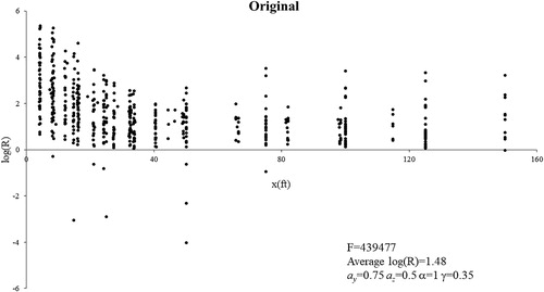
Fig. B2 Log of dilution ratio versus distance from the stack (With cutoff).

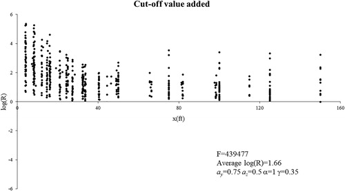
Fig. B3 Log of dilution ratio versus distance from the stack (Optimized with the variable γ).

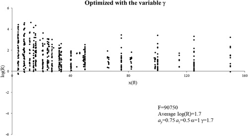
Fig. B4 Log of dilution ratio versus distance from the stack (Optimized with the variables α and γ).

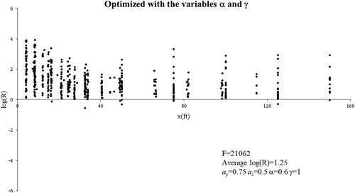
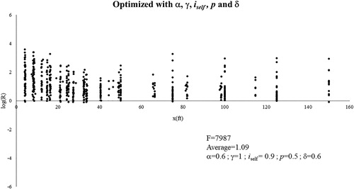
Fig. B5 Log of dilution ratio versus distance from the stack (Optimized with the variables α, γ, iself, p and δ).

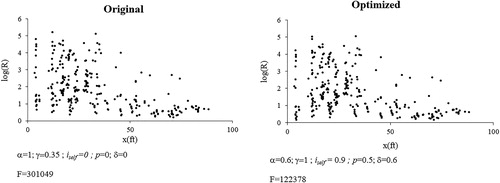
Finally, the optimized form of the model was checked on two other data sets; Wilson and Chui (1994) and Wilson and Lamb (1994) to make sure these values work for these data sets as well. These values were also checked to see how they work on tests with screens from ASHRAE RP 805 and tests from the receptors on the side wall (hidden intakes) from Schulman & Scire. The results are shown in the following Figures B6-B19.

1) Wilson and Chui (1994)

Fig. B6 Original and optimized dilution predictions for Wilson and Chui (1994).

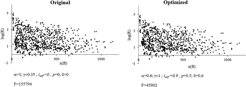
2) Wilson and Lamb (1994)

Fig. B7 Original and optimized dilution predictions for Wilson and Lamb (1994).

3) Petersen, Carter, and Ratcliff (1997) (Tests with Screens)

Fig. B8 Original and optimized dilution predictions for ASHRAE RP 805 (Tests with Screen).

4) Schulman and Scire (1991) (Hidden Intakes)

Fig. B9 Original and optimized dilution predictions for Schulman & Scire (Hidden Intakes).

References

- ASHRAE. 2019. ASHRAE handbook. Atlanta, GA: ASHRAE.
- Briggs, G. A. 1973. Diffusion estimation for small emissions. Atmospheric Turbulence and Diffusion Laboratory 83
- Cimorelli, A. J., S. G. Perry, A. Venkatram, J. C. Weil, R. J. Paine, R. B. Wilson, R. F. Lee, W. D. Peters, and R. W. Brode. 2005. AERMOD: A dispersion model for industrial source applications. Part I: General model formulation and boundary layer characterization. Journal of Applied Meteorology 44 (5):682–93. doi:10.1175/JAM2227.1
- Gupta, A., T. Stathopoulos, and P. Saathoff. 2012. Evaluation of ASHRAE dilution models to estimate dilution from rooftop exhausts. ASHRAE Transactions 118 (1):1021–38.
- Hajra, B., T. Stathopoulos, and A. Bahloul. 2011. The effect of upstream buildings on near-field pollutant dispersion in the built environment. Atmospheric Environment 45 (28):4930–40. doi:10.1016/j.atmosenv.2011.06.008
- Petersen, R. L., J. J. Carter, and M. A. Ratcliff. 1997. The influence of architectural screens on exhaust dilution. Final Report, ASHRAE
- Schulman, L. L., and J. S. Scire. 1991. The effect of stack height, exhaust speed, and wind direction on concentrations from a rooftop stack. ASHRAE Transactions 97 (2):573–85.
- Scrase, F. J. 1930. Some characteristics of eddy motion in the atmosphere. London: HM Stationery off.
- Teunissen, H. W. 1970. Characteristics of the mean wind and turbulence in the planetary boundary layer. (No. UTIAS-REVIEW-32). Toronto Univ Downsview (Ontario) Inst for Aerospace studies.
- Wilson, D. J., and B. K. Lamb. 1994. Dispersion of exhaust gases from roof-level stacks and vents on a laboratory building. Atmospheric Environment 28 (19):3099–111. doi:10.1016/1352-2310(94)E0067-T
- Wilson, D. J., and E. H. Chui. 1994. Influence of building size on rooftop dispersion of exhaust gas. Atmospheric Environment 28 (14):2325–34. doi:10.1016/1352-2310(94)90486-3
- Wilson, D. J., I. Fabris, J. Chen, and M. Y. Ackerman. 1998. Adjacent building effects on laboratory fume hood exhaust stack design. Final report of ASHRAE RP-897, February.
- Wilson, D.J. 2019. Phone interview with S. Shahvari and J. Clark.