Strategies to minimize SARS-CoV-2 transmission in classroom settings: combined impacts of ventilation and mask effective filtration efficiency

Abstract

Strong evidence exists indicating that aerosol transmission of the novel coronavirus SARS-CoV-2 is a significant transmission modality. We experimentally evaluated the impact of ventilation on aerosol dynamics and distribution along with the effective filtration efficiency (EFE) of four different mask types, with and without mask fitters, in a classroom setting. These were used to estimate aerosol conditional infection probability using the Wells–Riley model for three scenarios with different ventilation and mask interventions. Aerosol measurements confirmed that aerosol in the room was uniform within a factor of 2 for distances >2 m from the source. Mask EFE results demonstrate that most masks fit poorly with estimated leakage rates typically >50%. However, EFEs approaching the mask material FE were achievable using mask fitters. Infection probability estimates indicate that ventilation alone is not able to achieve probabilities <0.01 (1%). The use of moderate to high EFE masks reduces infection probability, >5× in some cases. Reductions provided by ventilation and masks are synergistic and multiplicative. The results reinforce the use of properly donned masks to achieve reduced aerosol transmission of SARS-CoV-2 and other infectious diseases and motivate improvements in the EFE of masks through improved design or use of mask fitters.

1. Introduction

Foundational to infection control and prevention is a clear understanding of the modality of transmission of the contagion. For SARS-CoV-2, early during the COVID-19 pandemic, emphasis was placed on direct-contact and indirect-contact modes of transmission with recommendations focused on hand hygiene (WHO 2020c) and physical distancing (WHO 2020b); however, recognition of the long-range airborne route as a modality of transmission (Morawska and Milton 2020; CDC, 2020b; Nardell and Nathavitharana 2020; Morawska and Cao 2020; Morawska et al. 2021) means that appropriate intervention measures for infection control and prevention via airborne transmission are needed (Shen et al. 2021; Zhang 2020). A common approach for assessing long-range airborne transmission, referred to here as aerosol transmission, utilizes the Wells–Riley equation (Wells 1955; Riley, Murphy, and Riley 1978) to relate aerosol concentrations to infection probability assuming an exponential dose model (Noakes and Sleigh 2009). This approach has been applied widely for SARS-CoV-2, and other diseases (Riley, Murphy, and Riley 1978; Noakes and Sleigh 2009) for both prospective (Buonanno, Morawska, and Stabile 2020a) and retrospective analyses (Miller et al. 2020; Buonanno, Morawska, and Stabile 2020a), with a particular focus on super-spreader events (Miller et al. 2020; Lu et al. 2020).

1.1. Wells–Riley model

The application of the Wells–Riley equation to a simple well-mixed room control-volume model (often termed a box model) is useful for risk assessment and planning of interventions. Use of this approach requires information on the setting of the event (room and heating ventilation and air conditioning (HVAC) system information), event duration, the potential emission rate of infectious aerosol and breathing rates of susceptible individuals, and information on interventions being considered (Riley, Murphy, and Riley 1978; Gammaitoni and Nucci 1997). Of these parameters, the emission rate of infectious aerosol tends to be the most uncertain, although recent work has better defined the range of values to consider for SARS-CoV-2 (Buonanno, Stabile, and Morawska 2020a, 2020b). The next most uncertain parameters are related to potential interventions such as increasing the room ventilation rate and the filtration efficiency of masks donned by individuals. Finally, the well-mixed approximation potentially adds significant uncertainty to any estimates using the Wells–Riley model.

The Wells–Riley model has been used in the past to understand the impact of different interventions intended to reduce the risk of aerosol disease transmission (for different diseases) and the relative risk of different scenarios. For example, investigators have used the approach to study the impacts of exposure duration, breathing and quanta emission rates, HVAC air change rate and particle filtration, respirators and masks, UV degradation, and particle deposition (Azimi and Stephens 2013; Gammaitoni and Nucci 1997; Fennelly and Nardell 1998; Nazaroff, Nicas, and Miller 1998; Buonanno, Morawska, and Stabile 2020a; Miller et al. 2020), as well as other factors. With regards to increasing HVAC air changes per hour and/or HVAC particle filtration, previous work has shown decreasing transmission probabilities with increases in these parameters (Fennelly and Nardell 1998; Azimi and Stephens 2013; Fisk et al. 2005; Miller et al. 2020). However, the dependence on air changes per hour (ACH) is modest for ACH >2. On the other hand, use of high efficiency respirators has been shown to significantly reduce probability of infection for airborne diseases like tuberculosis (Fennelly and Nardell 1998).

The Wells–Riley model has also been used to study SARS-CoV-2 transmission in classrooms, for examples see Foster and Kinzel (2021), Pavilonis et al. (2021), Shen et al. (2021) and Stabile et al. (2021). Foster and Kinzel compared estimates of infection probability based on CFD and a Wells–Riley model for a classroom space with mixing ventilation (MV) at two air change rates and found good agreement between the two approaches. Pavilonis et al. (2021) used a Wells–Riley model to estimate the aerosol transmission risk in New York City public schools for different exposure scenarios and found mean transmission probabilities (for all rooms considered) between 0.043 and 0.37, with the highest probabilities corresponding to transmission from teacher to students (neither wearing masks) for an exposure duration of 6.3 h. The Wells–Riley model was also used to look at the impact of ACH (Stabile et al. 2021; Shen et al. 2021) and other interventions (Shen et al. 2021; Zhang 2020) on transmission risk in classrooms for different scenarios.

1.2. Aerosols dynamics in indoor spaces

The behavior of aerosols in indoor spaces has seen significant study due to the impact of particulates on human health (for example see the reviews by Wallace (1996), Nazaroff (2004), and Tham (2016)) and the potential for bioaerosols to result in disease transmission (Morawska 2006; Zhu, Kato, and Yang 2006). Recent work has focused on the dispersal and dynamics of aerosol particles in indoor spaces related to the spread of SARS-CoV-2 (Kohanski, Lo, and Waring 2020; Nissen et al. 2020; Smith et al. 2020; Somsen et al. 2020a, 2020b). It is well known from these, and other studies, that ventilation and airflow within a room impact aerosol concentration and transport (Nazaroff 2004; Zhu, Kato, and Yang 2006; Lu et al. 2020; Nissen et al. 2020; Van Der Steen et al. 2017). Room air-exchange rates vary significantly based on the type of building and specific location (Nazaroff 2004), with the majority of residences and offices in the US having air-exchange rates <3 ACH (Nazaroff 2004). Although widely studied, there is still a lack of information on aerosol dynamics and distribution measurements in conventionally high-occupant density spaces in the bioaerosol size range relevant for aerosol transmission of COVID-19.

1.3. Mask filtration efficiency

In addition to increasing ventilation rate, it is now recognized that it is critical for the general public who are not vaccinated to wear masks in indoor environments and outdoors when physical distancing may not be achievable (CDC 2020a; WHO 2020a). Evidence from work by Ueki et al. (2020) and Leung et al. (2020) demonstrating the ability of masks to reduce virus emission and transmission via aerosols, and real world examples of masks preventing transmission of the virus when masks are consistently worn (Hendrix et al. 2020; Wang et al. 2020), both strongly support the use of masks. However, the effectiveness of a masks depends strongly on the material filtration efficiency (MFE) and fit of the mask to the user’s face (van der Sande, Teunis, and Sabel 2008; Hill, Hull, and MacCuspie 2020; Mueller et al. 2020), which can result in an effective filtration efficiency (EFE) that is much lower than the MFE.

The filtration performance of materials for both homemade cloth masks and commercially produced masks (cloth masks, disposable non-medical masks, medical masks, and KN95 and N95 masks) has been studied both before the COVID-19 pandemic (Davies et al. 2013; Jang Ji and Kim Seung 2015; Jung et al. 2014; Rengasamy, Eimer, and Shaffer 2010; van der Sande, Teunis, and Sabel 2008) and during (Bagheri et al. 2021; Crilley et al. 2021; Drewnick et al. 2021; Hill, Hull, and MacCuspie 2020; Hao et al. 2020, Hao, Xu, and Wang 2021; Joo et al. 2021; Kelly et al. 2020; Konda et al. 2020b; Lindsley et al. 2021a, 2021b; Long et al. 2020; Mueller et al. 2020; Pan et al. 2021; Teesing et al. 2020; Whiley et al. 2020; Zhao et al. 2020) (also see the recent review by Clase et al. (2020)). However, the particle size range of the measurements, filtration conditions, and testing equipment and methods vary greatly between studies, making comparisons difficult.

Most studies have focused on measurements at small particle sizes (<1 μm) similar to the range of sizes achieved with the NaCl aerosol used for certification of N95 respirators (count median diameter of 0.075 ± 0.02 μm and a standard geometric deviation not exceeding 1.86 (42 CFR Part 84 84 2021)) (Crilley et al. 2021; Hao et al. 2020, Hao, Xu, and Wang 2021; Joo et al. 2021; Lindsley et al. 2021a; Long et al. 2020; Rengasamy, Eimer, and Shaffer 2010) or do not have size-resolved measurements (Davies et al. 2013; Long et al. 2020; Kelly et al. 2020; Lindsley et al. 2021a; Long et al. 2020; Mueller et al. 2020). A few studies have investigated a wider range of particle sizes with size-resolved measurements for sizes up to 10 μm (Bagheri et al. 2021; Drewnick et al. 2021; Konda et al. 2020b; Pan et al. 2021). Filtration face velocities studied vary from 0.78 cm/s (Hill, Hull, and MacCuspie 2020) to 16.5 m/s (Kelly et al. 2020) with the majority of studies having face velocities in range of 2–25 cm/s (Bagheri et al. 2021; Crilley et al. 2021; Drewnick et al. 2021; Hao et al. 2020, Hao, Xu, and Wang 2021; Joo et al. 2021; Lindsley et al. 2021a; Long et al. 2020; Pan et al. 2021; Rengasamy, Eimer, and Shaffer 2010).

Studies generally measure both particle penetration (i.e. filtration efficiency) and pressure drop, although instrumentation and the method of generating the challenge aerosol can vary significantly. The majority of studies have used NaCl aerosols, although some have utilized ambient aerosol particles (Bagheri et al. 2021; Drewnick et al. 2021; Teesing et al. 2020). The NaCl aerosols are typically dried and diluted. In some instances, they have been charge neutralized to a Boltzmann equilibrium state, usually in conjunction with the use of an automated filter tester (e.g. TSI 8130A0) (Jung et al. 2014; Lindsley et al. 2021a; Rengasamy, Eimer, and Shaffer 2010; Zhao et al. 2020). The influence of mask fit and mask leakage has also been studied using fit testing (Davies et al. 2013; Lindsley et al. 2021a, 2021b; Mueller et al. 2020; Teesing et al. 2020; van der Sande, Teunis, and Sabel 2008) and simulated leakage (Drewnick et al. 2021; Konda et al. 2020b). The study of Pan et al. (2021) is notable as it measured the influence of mask fit for both inhalation and exhalation using two head forms facing each other, separated by 33 cm (mouth-to-mouth), along with measurements of MFE (albeit at a different face velocity). Hill, Hull, and MacCuspie (2020) also did measurements with a mask on a head form, but only for inhalation.

Even with the differences in methods and filtration conditions, there are several consistent findings amongst studies. Firstly, the MFE of cloth mask materials (knit and woven cotton and non-woven polypropylene) has been found to be relatively low for a single layer for particle sizes of 0.3–0.5 μm with typical values in the range of 2–25% and corresponding filter quality factors ($q_F=-\hspace{0.17em}\text{ln}\hspace{0.17em}(1-{\eta }_f)/\Delta P,$ where η_f is the MFE and $\Delta P$ is the pressure drop) ranging from q_F = 0.0002 to 0.007 Pa^–1 (Crilley et al. 2021; Bagheri et al. 2021; Drewnick et al. 2021; Hao et al. 2020; Joo et al. 2021; Pan et al. 2021; Rengasamy, Eimer, and Shaffer 2010). An exception to this is the work of Konda et al. (2020b) which found very high filtration efficiency of 90–95% for woven cotton of different thread counts. This result appears to be in error given the later correction to the article which indicated that flow rates were not controlled for the experiments, therefore, this result should be discounted (Konda et al. 2020a). Zhao et al. (2020) found a substantially higher filter quality factor for a polypropylene spunbound interfacing material ($q_F=$ 0.040 Pa^–1) when considering all particle sizes, but given the lack of size-resolved results (no direct comparison for 0.3–0.5 μm is available) and relatively high uncertainties in the pressure drop and filtration efficiency used to determine the quality factor, this can also be considered a potential outlier. Lindsley et al. (2021a) studied a range of commercially produced cloth masks with a TSI 8130 automated filter tester using a modified version of the NIOSH standard test procedure (NIOSH 2019). They found overall MFEs in the range of 10–20% for cloth masks (Lindsley et al. 2021b).

Previous work has demonstrated the impact of mask fit on the EFE of masks, with high MFE masks exhibiting poor EFE at times to due to the impact of mask fit (Davies et al. 2013; Hill, Hull, and MacCuspie 2020; Lawrence et al. 2006; Lindsley et al. 2021a; Mueller et al. 2020; Pan et al. 2021; van der Sande, Teunis, and Sabel 2008). Pan et al. (2021) generally found similar EFEs for both inhalation and exhalation for most masks tested, although a few masks showed significantly different EFEs for inhalation and exhalation with the exhalation EFE typically being higher. Hill, Hull, and MacCuspie (2020) demonstrated that when actively sealed to the head form used filtration efficiencies very close to the MFE of the mask were achieved. Several studies have also demonstrated the improvement in fit (i.e. improved EFE) achieved when using external devices to assist in fitting masks to the user’s face (Brooks et al. 2021; Clapp et al. 2021; Mueller et al. 2020; Hill, Hull, and MacCuspie 2020).

Overall, there is a general lack of data at appropriate filtration conditions (corresponding to normal breathing rates, i.e., face velocities of 0.5–3 cm/s) that is size resolved, covers the entire range of interest for human produced bioaerosols (from approximately 200 nm to 10 μm), and that considers the impact of mask fit in specific realistic settings. The current work addresses these issues for the specific setting of a classroom with physical distancing.

1.4. Human respiratory aerosols

In this work, we define inhalable virus laden aerosol particles (bioaerosols) as being in the 100 nm–5 μm size range for several reasons. First, aerosol particles in this size range have been demonstrated to carry viable SARS-CoV-2 (Chia et al. 2020). Second, they are consistent with the particle sizes humans generate by common activities in a classroom that include breathing, speaking, singing, coughing, and sneezing (Morawska et al. 2009; Johnson et al. 2011; Alsved et al. 2020). Third, these aerosol particles readily breach the current 2-m physical-distancing guidelines due to their ability to remain airborne for extended periods of time and to be carried by air currents in the indoor environment. Respiratory droplets less than 10 μm in size rapidly (<1 s) reach an equilibrium diameter about one-half their original diameter due to evaporation and equilibration at the ambient conditions (Nicas, Nazaroff, and Hubbard 2005; Holmgren et al. 2011; Alsved et al. 2020; Kohanski, Lo, and Waring 2020). Therefore, the size range considered corresponds to droplets at the point of emission ranging in size from 200 nm to 10 μm and to an equilibrium particle size range from 100 nm to 5 μm, consistent with the size range described by Fennelly (2020).

1.5. Paper focus

The focus of this paper is to provide experimental measurements that reduce the uncertainties of model inputs and approximations for the Wells–Riley model applied to a classroom setting, and to study the impact of specific interventions (ventilation rate and mask filtration efficiency) on aerosol conditional infection probabilities using the model. In this work, we assume that measures have already been put in place to reduce occupant density and to control short-range droplet and fomite transmission. Aerosol dynamics and distribution measurements were performed to assess the impact of HVAC ventilation rates on aerosol concentrations and to quantify the loss rates of particles. Mask effective filtration efficiency measurements were performed for four mask types with and without the use of two different mask fitters. Providing information on the impact of mask fit on EFE. Estimates of conditional infection probability were performed using the measured ventilation parameters and mask EFEs as inputs to the Wells–Riley model for three instructor-student scenarios with different combinations of HVAC and mask interventions. A primary aim of this paper is to provide insights regarding the effectiveness of masks and ventilation interventions, and combinations thereof, for reducing the likelihood of COVID-19 aerosol transmission (and other airborne diseases) in traditionally high occupancy spaces such as classrooms.

2. Methods and materials

2.1. Estimating conditional infection probability

The Wells–Riley equation (Riley, Murphy, and Riley 1978) predicts the conditional probability of infection, P, based on a susceptible individual inhaling an infectious quanta dose, D_q, during the duration of an event, where (1) $$P=1-\hspace{0.17em}\text{exp}\hspace{0.17em}\left(-D_q\right).$$(1)

A single infectious quantum dose is related to the number of bioaerosol particles (and number of viable virus copies) inhaled that results in a conditional probability of infection of $P=1-\hspace{0.17em}\text{exp}\hspace{0.17em}(-1)$ = 63.2%.

The efficacy of the equation for predicting infection probability is based on how well the underlying assumptions hold. These assumption include (Noakes and Sleigh 2009): the virus incubation period $\gg$ timescale for the event, a single large dose is equivalent to multiple small doses over a period of time, and probabilistic approach, best suited to large populations. The first two assumptions may hold well for many scenarios for SARS-CoV-2 in high-risk settings of limited exposure duration (on the order of hours). The third assumption is related to the limits of deterministic application of the model to situations with small numbers of individuals.

Estimation of infection probability due to airborne transmission requires calculation of the evolution of bioaerosol concentration in the space of interest in order to estimate the number of infectious quanta a susceptible individual inhales. The Wells–Riley equation is typically utilized by applying a well-mixed room approximation using a simple control-volume model (referred to collectively as the Wells–Riley model), as was done by Riley, Murphy, and Riley (1978), and is subject to several other assumptions (Noakes and Sleigh 2009). In the case of an infectious individual(s) present in the room, the concentration we are interested in is the concentration of infectious aerosol, for measurements presented in the paper focused on the efficacy of different interventions, NaCl aerosol was seeded into the room to perform evaluations of aerosol distributions and dynamics and mask filtration efficiency. For those cases, we are interested in describing the evolution of the concentration of NaCl particles in the room (derivation of equations for this are provided in the Supplemental Information).

2.1.1. Infectious quanta number density and dose

In the case of an infectious individual for the Wells–Riley equation, the dose in Equation 1(1) $$P=1-\hspace{0.17em}\text{exp}\hspace{0.17em}\left(-D_q\right).$$(1) is a function of the total net emission rate of infectious quanta $\dot{Q}$ that determines the number density of infectious quanta in the room (n_q) as a function of time, that is, (2) $$n_q=\frac{\dot{Q}}{{\lambda }_q{V}_R}\left[1-\left(1-\frac{n_{q_0}{\lambda }_q{V}_R}{\dot{Q}}\right)\hspace{0.17em}\text{exp}\hspace{0.17em}(-{\lambda }_{q}t)\right]$$(2) where λ_q is the total first-order loss rate for quanta in the room, V_R is the room volume, and $n_{q_0}$ is the initial quanta concentration at the start of the exposure duration. The net total emission rate of quanta $\dot{Q}$ is related to the individual quanta emission rate $\dot{q}$ by (3) $$\dot{Q}=N_I\dot{q}\left(1-{\eta }_{f,M_{\mathit{exh}}}\right)$$(3) where N_I is the number of infectious individuals in the room (usually assumed to be 1) and ${\eta }_{f,M_{\mathit{exh}}}$ is the EFE of masks worn by individuals in the room during exhalation. The net total quanta emission rate defined in this way enables the use of masks to be explicitly included in the analysis.

The infectious quantum dose, D_q, is determined by multiplying the average number density of quanta in the room (${\overline{n}}_q$) during an event and the breathing rate of susceptibles (${\dot{V}}_b$) in the room by the duration of the event (t_D) (4) $$D_q={\overline{n}}_q{\dot{V}}_b{t}_D\left(1-{\eta }_{f,M_{\mathit{Inh}}}\right)$$(4) where number of quanta inhaled (dose) is written to take into account the EFE during inhalation (${\eta }_{f,M_{\mathit{Inh}}}$) of masks worn by susceptible individuals in the room. In the current study, the infectious quanta is assumed to be SARS-CoV-2.

The average concentration of quanta in the room (${\overline{n}}_q$) is determined from integration of Equation 2(2) $$n_q=\frac{\dot{Q}}{{\lambda }_q{V}_R}\left[1-\left(1-\frac{n_{q_0}{\lambda }_q{V}_R}{\dot{Q}}\right)\hspace{0.17em}\text{exp}\hspace{0.17em}(-{\lambda }_{q}t)\right]$$(2) over the time period of interest. For the simplified case with no infectious quanta initially present in the room at the start of the event duration of interest, integration of Equation 2(2) $$n_q=\frac{\dot{Q}}{{\lambda }_q{V}_R}\left[1-\left(1-\frac{n_{q_0}{\lambda }_q{V}_R}{\dot{Q}}\right)\hspace{0.17em}\text{exp}\hspace{0.17em}(-{\lambda }_{q}t)\right]$$(2) gives (5) $${\overline{n}}_q=\frac{\dot{Q}}{{\lambda }_q{V}_R}\left(1-\frac{1}{{\lambda }_q{t}_D}\left[1-\hspace{0.17em}\text{exp}\hspace{0.17em}(-{\lambda }_q{t}_D)\right]\right).$$(5) The loss rate λ_q includes mechanisms for particle removal and also a loss term for virus inactivation (k), that is, (6) $${\lambda }_q={\lambda }_{FA}+{\lambda }_f+{\lambda }_{TS}+k$$(6) where λ_FA represents the dilution effect of fresh air, λ_f accounts for the removal of quanta due to filtration (central and in-room systems would be additive, as applicable), λ_TS is the loss due to quanta settling in the room or due to HVAC system deposition. Additional loss mechanisms that may be applicable to a given situation can be added to Equation 6(6) $${\lambda }_q={\lambda }_{FA}+{\lambda }_f+{\lambda }_{TS}+k$$(6) .

An approximate expression can be derived for the limiting case where D_q is small (i.e. $D_q\le$ 0.2) and a steady-state value of quanta in the room is assumed. Substituting for D_q and ${\overline{n}}_q$ using Equations 4(4) $$D_q={\overline{n}}_q{\dot{V}}_b{t}_D\left(1-{\eta }_{f,M_{\mathit{Inh}}}\right)$$(4) and 5(5) $${\overline{n}}_q=\frac{\dot{Q}}{{\lambda }_q{V}_R}\left(1-\frac{1}{{\lambda }_q{t}_D}\left[1-\hspace{0.17em}\text{exp}\hspace{0.17em}(-{\lambda }_q{t}_D)\right]\right).$$(5) , and for $\dot{Q}$ using 3 we have (7) $$P\approx \frac{N_I\dot{q}}{\lambda V_R}{\dot{V}}_b{t}_D(1-{\eta }_{f,M_{\mathit{Inh}}})(1-{\eta }_{f,M_{\mathit{Exh}}}).$$(7) In this limit, the conditional infection probability is proportional to the quanta emission rate, the breathing rate of susceptibles, the duration of the exposure, and the product of the mask penetrations for inhalation and exhalation (penetration is equal to one minus the filtration efficiency (Hinds 1999)), and is inversely proportional to room volume and the first-order loss rate. If it is assumed that the susceptible and infectious individuals are wearing masks with the same EFE, then there is a squared dependence on mask penetration, this effect is stronger than the first-order loss coefficient that can be increased by increasing room ventilation. Derivation of the expressions in this section are provided in the Supplemental Information.

2.2. Classroom space studied

The classroom space used for the study measures 126.4 m² with a ceiling height of 2.870 m yielding a gross room volume of 362.6 m³. The room is served by a central-station variable air volume (VAV) air handling unit equipped with MERV 15 filtration which serves multiple spaces in the building including classrooms, offices, common areas, and lab spaces. Each individual space within the building is equipped with one or more VAV boxes that modulate supply air to the room in response to load changes. Because the central-station air handling unit’s maximum and minimum air flowrates (88,900 m³/h and 28,000 m³/h, respectively) are much larger than the air flowrate to an individual room, significant dilution occurs prior to recirculation back to the space. The air handling unit’s outdoor airflow rate ranges from a minimum of 20,261 m³/h to 88,900 m³/h.

The classroom space studied is representative of many classrooms in the building that all utilize a MV system. It has a single VAV box that supplies conditioned air to four 4-way throw fixed area overhead diffusers arranged in a rectangular layout. A single overheard return is located in the rear corner of the room. Air delivery supplied to the room by the four-way throw fixed area diffusers exits the diffusers with sufficient velocity, at a small angle relative to the room ceiling, such that air within the room mixes with it via the Coanda effect. This tempers the lower temperature supply air before reaching the occupied portion of the space. The mixing process at each diffuser and the well-spaced rectangular arrangement of the diffusers is designed to result in a room that is well-mixed (typical of MV (Zhang 2020)), ensuring occupant comfort. Although the room supply and return air layout is focused on mixing for occupant comfort, it has the collateral effect of mixing any contaminants that may be present or generated within the space.

The minimum and maximum total air flowrates for the classroom where testing was conducted ranged from 487.6 m³/h to 1832 m³/h, corresponding to air change rates of 1.34 ACH and 5.05 ACH. The fraction of outdoor air varied from approximately 72% at the low air change rate to 23% at the high air change rate.

Normally, this room accommodates 48 students and a single instructor giving an occupant density of 2.58 m²/person (an image of the space in its pre-COVID-19 configuration is shown in Figure 1); however, the room layout was modified with a nominal 2.13 m separation distance between students and a 3.05 m buffer separation between the instructor and seated students in response to COVID-19. This reconfiguration of the room reduced occupant capacity to 17 (16 students and one instructor) decreasing the occupant density to 7.43 m²/person. Figure 2a shows a plan view of the reduced occupant density classroom along with relative layout of the room’s HVAC supply and return. In the schematic each student desk is occupied by a single student.

Fig. 1. Photo showing the classroom space used as a testbed for the current study (in a pre-COVID-19 layout).

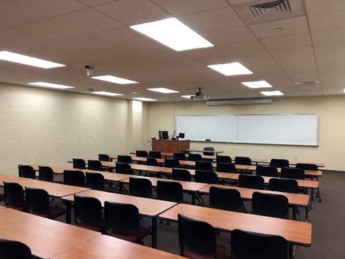
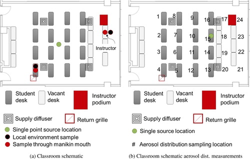
Fig. 2. (a) Schematic of the classroom layout used as a testbed for the current study, showing the locations of desks where student manikins were located (student desk), additional desks that were empty (vacant desk), the instructor podium at the front of the room, and the supply diffusers and return and (b) classroom layout showing setup for mapping distribution of concentration within the classroom. Number locations indicate positions where aerosol concentration was measured. Location of single student manikin emitting aerosol during the measurements is indicated by a green dot.

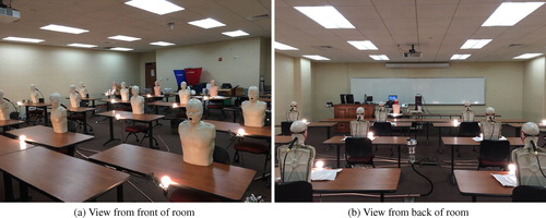
To simulate occupants within the room during testing, 17 CPR manikins were deployed and positioned at each of the 16 student locations with the 17th manikin positioned at the front of the room where an instructor would be. The CPR manikins were modified to enable a 25.4-mm outside diameter (19.05-mm inside diameter) piece of conductive silicon tubing to be passed through the back of the manikin heads with the exit of the tube filling the manikins’ open mouths. This tube was connected to either the aerosol sampling instruments or to an aerosol source. Each student location also had an incandescent (75 W) lightbulb co-located to simulate sensible heat load from classroom occupants. Light bulbs were turned on during all testing performed for the work. Images of the full-scale experimental setup are shown in Figure 3. Additional details on the room and experimental setup are provided in the Supplemental Information.

Fig. 3. Classroom space setup with manikins (a) view from the front of the room looking back and (b) from the back of the room looking forward.

2.3. Aerosol generation and measurement

Aerosol testing was conducted in the classroom to: (1) assess validity of the well-mixed assumption in the Wells–Riley model, (2) evaluate the rate of concentration build-up/decay and loss rates of particles, and (3) obtain data on the EFE of various masks as worn by occupants. A polydisperse NaCl (salt) aerosol was generated by atomizing a 20% by weight solution of NaCl and distilled water using an aerosol generator (TSI 3076) with a nominal airflow rate of 3 ± 0.5 SLPM. Output of the aerosol generator was dried using a diffusion dryer (TOPAS DDU 570/H) followed in series by two aerosol neutralizers (both TSI 3077s). Following drying and charge neutralization, an axial diluter was used to reduce particle concentration and to achieve the desired total aerosol flowrate. Use of a charge neutralized aerosol provides a more conservative estimate of mask EFE relative to the use of an unneutralized aerosol. Total aerosol flow was varied based on the number of manikins (or sources) setup to emit aerosol to the room.

Three different types of aerosol measurement instruments were used to measure size-resolved concentrations at discrete locations within the classroom and through the mouths of the manikins. The three instrument types included an electrical low-pressure impactor (ELPI, Dekati) and an aerodynamic particle sizer (APS, TSI 3321), which both classify particle size based on a particle’s aerodynamic diameter, and two optical particle sizers (OPS, TSI 3330), which size particles individually based on light scattering. For size-resolved information the ELPI and APS results were typically used. Aerodynamic diameter was estimated for the OPS instruments based on comparison with ELPI size distributions and finding a single diameter scaling factor that gave the best agreement between distributions. Equipment specifications are provided in the Supplemental Information.

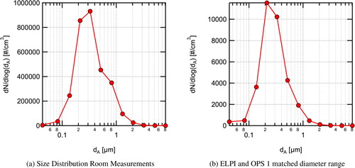
A representative NaCl particle size distribution, generated with a dilution airflow rate of 120 ± 12 SLPM and measured by the ELPI, is shown in Figure 4a. The distribution has a count median diameter (CMD) of 0.25 μm, a geometric mean diameter (GMD) of 0.34 μm, and a geometric standard deviation (GSD) of 1.86. Particle sizes with significant concentrations range from 0.043 μm to approximately 3.2 μm in aerodynamic diameter. The size distribution is not perfectly log-normal and appears to have two modes (one centered around 0.25 μm and a second around 0.8 μm) as indicated by the bump on the right-hand side of the distribution. The range of particle sizes tested in the current work is representative of the typical size range of aerosol particles emitted while breathing, speaking, and coughing. However, the concentration of the aerosol used is several orders of magnitude higher than emitted during breathing, speaking, or coughing, in order to discriminate the NaCl aerosol from background aerosol concentrations in the room.

Fig. 4. a. NaCl aerosol size distribution as a function of aerodynamic diameter (d_A) generated by the aerosol generator measured directly after dilution. b. NaCl aerosol size distribution measured with the ELPI during filtration efficiency measurements measured at position 4 in Figure 2b after steady-state was reached. Error bands representing uncertainty due to random variations during the averaging interval are smaller than the symbols used and are not visible in the plot.

2.4. Aerosol dynamics and distribution

2.4.1. Aerosol dynamics

Aerosol was dispersed from a source at the center of the room, exiting upward from a 152-mm diameter duct at an exit height of 0.97 m with a velocity of 6.15 cm/s (jet Reynolds number = 576). Time-resolved and size-resolved aerosol concentration measurements were performed at the front and rear of the room. Aerosol measurements at the front of the room were made near the instructor position (see Figure 2a) at a height of 1.2 m. Sampling was performed with the APS and ELPI through their vertically oriented instrument inlets. Sampling in the rear of the room was performed near the overhead air return grille. Two OPS instruments were used at this location sampling at a height of 1.2 m through their vertically oriented instrument inlets. Sampling with two instruments at each location enabled a consistency check between the instruments. A balometer (TSI Alnor) was used to measure return and supply air flowrates at the start and end of each test.

A second experiment evaluated the steady-state room aerosol concentrations at lower and higher room supply air-exchange rates. Aerosol was seeded steadily into the room through the mouths of 15 non-sampling student manikins (to provide a relatively uniform distribution in the room) for a duration greater than four times the time constant for the low flow rate of 1.34 ACH ($\tau =1/\lambda$) bringing the room aerosol concentration to steady-state as measured by the ELPI. Once steady-state was reached, the airflow supplied to the room by the HVAC system was increased to 5.05 ACH by biasing the room thermostat using a local heat source and the time evolution of the decrease in aerosol concentration was measured.

2.4.2. Aerosol spatial distribution

Measurements of the aerosol spatial distribution in the room were acquired to assess the accuracy of the well-mixed room approximation in the Wells–Riley model. For these measurements, aerosol was seeded steadily into the room for a duration greater than four times the time constant for buildup of aerosol concentration in the room, resulting in an approximately steady-state aerosol distribution. Size-resolved aerosol measurements were made at locations adjacent to each student position and at probable instructor locations (location are indicated by numbers in Figure 2b) using OPS1.

2.5. Effective filtration efficiency

Four masks designed to cover the nose and mouth with the intent of providing respiratory particle protection were evaluated. The masks tested included a commercial 4-ply knit cotton mask, a 3-ply spunbond polypropylene (ADO Products, Pro Pac Insulation Fabric) mask designed by the UW-Madison emergency operations committee (EOC) and produced by a local custom sewing manufacturer for UW-Madison (Laacke & Joys Design & Manufacturing) referred to as the EOC mask throughout, a 3-ply disposable non-medical mask with a melt-blown polypropylene center ply (Hodo, single-use mask) referred to as a procedure mask throughout, and an ASTM F2100 (ASTM 2019) level-2 rated medical surgical mask (Medicom, SafeMask FreeFlow). All masks except for the 4-ply knit cotton mask had a formable metal nose strip. Although not an exhaustive list, these four masks are representative of a relatively broad range of filtration performance that individuals may have access to. The surface of the hard plastic CPR manikin’s face was modified to be slightly compliant to better represent a human’s face. Images of the masks as installed on the manikins for filtration measurements are provided in the Supplemental Information along with more information on modification of the manikin’s face.

Measurements were performed with masks fit in a way that is representative of someone intent on effective use of the mask, that is, covering the nose and mouth completely and with the formable nose piece (if present) shaped to the manikin’s face. Additionally, an adjustable mask ear saver (Seljan Company, https://earsaver.net/) was used to allow the masks to be pulled tight to the manikin’s face. The fit of the masks was close to the best achievable with each individual mask by itself. Even when fit well, some gaps near the nose bridge and on the sides and bottom of the mask were visible resulting in leakage around the mask. This was particularly true for the knit cotton mask which did not have a formable nose piece and for the procedure mask whose nose piece did not maintain its shape well after forming.

We also evaluated the use of two mask fitters, one developed in collaboration with Lennon Rodgers at the UW-Madison Makerspace (Badger Seal, https://making.engr.wisc.edu/mask-fitter/) and a second commercial mask fitter (Fix the Mask (FTM) mask brace, https://www.fixthemask.com/). The mask fitters are designed to seal a mask to the user’s face to minimize leakage around the mask; potentially enabling the full filtration potential of the mask to be reached. Use of mask fitters requires that the masks used have reasonably low pressure drop at typical breathing flowrates. All of the mask materials used here fulfill that requirement with pressure drops <40 Pa for a face velocity of 3.5 ± 0.5 cm/s (as measured in separate experiments with a 25.4 mm diameter flow area), equivalent to a full mask flowrate of 28.3 L/min. Images of the mask fitters installed on the manikin with the EOC mask and data on the MFE of the masks used are provided in the Supplemental Information.

Mask aerosol leakage makes estimating infection probabilities using the Wells–Riley model highly uncertain when trying to take into account the effective mask filtration efficiency. We define EFE as the filtration efficiency of the mask as worn by the user. This is lower than the mask MFE which only considers the flow going through the mask material. In reality, given the pressure drop across the mask filtration material it is expected that in normal mask wear a large fraction of the flow will go out the sides of the mask, significantly decreasing the filtration efficiency as worn, that is, the effective mask filtration efficiency. A simple estimate of the leakage velocity for a relatively low mask pressure drop of 20 Pa ($v=\sqrt{(2\Delta P)/\rho }$ from the Bernoulli equation) gives a potential leakage velocity of 5.9 m/s, which for a 1 cm² leakage area, would result in a leakage flow rate of 35 L/min (assuming a constant pressure drop). This flowrate is larger than the typical breathing flowrates associated with most activities (Adams 1993), indicating that if such a leakage path exists, most of the flow would follow that path and not go through the mask.

EFE measurements were made by seeding the room with the same polydisperse neutralized NaCl aerosol used for aerosol dynamics and distribution measurements. Room air was continuously seeded with aerosol during measurements. Measurements were not performed until the room aerosol concentration reached an approximate steady state (>3 time constants after initiating seeding at 1.34 ACH). The aerosol particle size distribution in the room measured by the ELPI after steady state had been reached in the room is shown in Figure 4b. The distribution shown here was measured in the back of the room near the return grille (position 4 in Figure 2b), whereas the distribution shown previously in Figure 4a was the distribution supplied to the room.

EFE for inhalation was tested by sampling air from the room through the 19.05-mm inside diameter conductive silicone tube installed in the manikin’s mouth connected via a brass hose fitting reducer to a 6.35-mm inside diameter conductive silicon tube connected to the inlet of the ELPI. The entire sample was sent to the ELPI with a sample flowrate of 9.7 LPM. This flowrate rate is similar to inhalation rates for sitting and/or standing for adults (Adams 1993). Typical mask flow areas for this work were approximately 100–200 cm², assuming even flow across this area gives estimated face velocities of between 0.8 and 1.6 cm/s which are significantly lower than what has been used in almost all mask MFE studies listed in Section 1.3. All measurements were performed with the ELPI using the following procedure: (1) sample room air for 4 min without a mask, (2) install mask on the manikin, (3) sample room air through the mask on the manikin for 4 min after flow equilibrates (∼1 min), (4) remove mask from the manikin, and (5) sample room air for 4 min without a mask.

For the size-resolved measurements, filtration efficiency for each particle size is given by (8) $${\eta }_{f,M_{\mathit{Inh}}}=1-\frac{2{\overline{n}}_M(d_A)}{{\overline{n}}_R^B(d_A)+{\overline{n}}_R^A(d_A)}$$(8) where ${\overline{n}}_M(d_A)$ is the average number density of particles at aerodynamic diameter (d_A) measured with the mask on the manikin, and ${\overline{n}}_R^B$ and ${\overline{n}}_R^A$ are the average number densities measured before and after with the mask off (representing the room concentration). Uncertainty in the filtration efficiency determined using Equation 8(8) $${\eta }_{f,M_{\mathit{Inh}}}=1-\frac{2{\overline{n}}_M(d_A)}{{\overline{n}}_R^B(d_A)+{\overline{n}}_R^A(d_A)}$$(8) was estimated using first-order uncertainty propagation. Uncertainty estimates include contributions due to random measurement variation during the averaging period, bias due to drift in the room concentrations, and bias estimates based on potential zero drift for each channel on the ELPI assuming a maximum zero current drift of ±2.5 fA (see the Dekati ELPI manual for converting this to a number density for each size bin).

Total filtration efficiency was calculated using Equation 8(8) $${\eta }_{f,M_{\mathit{Inh}}}=1-\frac{2{\overline{n}}_M(d_A)}{{\overline{n}}_R^B(d_A)+{\overline{n}}_R^A(d_A)}$$(8) with the size-resolved number densities replaced with the total number densities. Uncertainty was calculated in the same fashion as the size-resolved measurements with the only difference being that instead of using an assumed current drift for the zero bias, the zero bias was assumed to have a maximum number density value of 150 cm⁻³ based on observations during the measurement campaign.

3. Results and discussion

3.1. Aerosol dynamics and distribution

3.1.1. Aerosol dynamics

The transient response of the classroom aerosol concentration during buildup and a subsequent decay at the two measurement locations is shown in Figure 5. Data collection started 5 min before the initiation of aerosol seeding at 10:20 am from the single centrally-located seeding position (shown in Figure 2a). Aerosol was seeded at an approximately constant rate for 1 h after which the aerosol flow was stopped. During the period where data were collected, the supply airflow to the classroom averaged 488 m³/h (1.34 ACH). After the aerosol flow was stopped at 11:20 am, the air exchange in the room and settling reduced the aerosol concentration in the room.

Fig. 5. Aerosol concentration in the classroom during buildup of aerosol from a single source located at the center of the room and during the decay of aerosol following shutoff of the aerosol source. a. Aerosol concentrations normalized by their peak value for all four instruments used; and b. Measured time-resolved aerosol concentrations in the front and rear of the room for a similar range of diameters. Aerosol seeding was started at 10:20 am and stopped at 11:20 am. Measurements are for approximately matched size ranges from ∼0.7 μm to 10 μm.

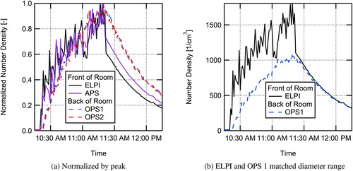
Once the aerosol was turned on at 10:20 am, the instruments at the front of the room saw an abrupt increase in aerosol concentration followed by a somewhat noisy, approximately exponential (i.e. $\propto 1-\hspace{0.17em}\text{exp}\hspace{0.17em}(-\lambda t)$) rise in concentration. The OPS instruments at the rear of the room, near the air return, showed a much smoother rise in aerosol concentration. This indicates some level of non-uniformity in the spatial aerosol distribution and that the aerosol is more uniformly mixed in the rear location. This is likely due to the proximity of the rear sampling location to the air return. Once the aerosol source was turned off, the concentration decay for both instruments at the front of the room is almost completely smooth. Perhaps more interesting is that the absolute total concentrations shown in Figure 5b for the ELPI and OPS1 are very similar in magnitude for a similar measurement size range, indicating that the distribution in the room becomes nearly uniform relatively quickly with the aerosol source turned off, and the decay at both the front and rear of the room have nearly the same time constant for the same range of particle sizes.

Overall, the results for the single source at the center of the room suggest a relatively uniform buildup of aerosol concentration in the room with some local non-uniformity associated with turbulent fluctuations from the plume (Re_D = 576) being emitted at the center of the room. The fact that the difference in concentration between the front and back of the classroom varied but the differences were modest helps support the well-mixed assumption for the Wells–Riley model. This result is likely applicable to many classrooms that rely on MV similar to the space studied in this work. However, for spaces utilizing other air distribution methods, such as displacement or personal ventilation, the well-mixed approximation will most likely not be as accurate. Additionally, the size-resolved data (not shown) indicate that the loss rate for all particle sizes measured, during the period were the aerosol was shutoff, was similar with only modest size dependence seen in the loss rate.

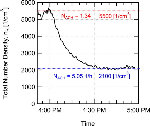
An additional run evaluated the steady-state room aerosol concentrations at lower and higher room air-exchange rates. Aerosol was seeded steadily into the room for a duration greater than four times the time constant for the low HVAC flow of 1.34 ACH, bringing the room aerosol concentration to steady-state as measured by the ELPI. Once a steady-state was reached, airflow supplied to the room was increased to 5.05 ACH. The factor of 3.8 increase in room air volume flow rate resulted in the average steady-state concentration decreasing from 5500 cm⁻³ to 2100 cm⁻³ based on ELPI measurements for the entire range of particle sizes measured at the instructor position. This decrease in aerosol concentration is shown in Figure 6.

Fig. 6. Decrease in aerosol concentration in the room when switching from low flowrate of 1.34 ACH to a high flowrate of 5.05 ACH while constantly seeding aerosol into the room. Measured with the ELPI for particle sizes from 0.043 μm to 10 μm.

Both the buildup of aerosol when seeding was first started with the HVAC flow at 1.34 ACH, and the decrease in aerosol when the HVAC flow was increased to 5.05 ACH were curve fit to the time-dependent concentration equation for a perfectly mixed room, similar to Equation 2(2) $$n_q=\frac{\dot{Q}}{{\lambda }_q{V}_R}\left[1-\left(1-\frac{n_{q_0}{\lambda }_q{V}_R}{\dot{Q}}\right)\hspace{0.17em}\text{exp}\hspace{0.17em}(-{\lambda }_{q}t)\right]$$(2) (see Supplemental Information). Fitting the rise in concentration for the ELPI data gave a value of the first-order particle loss rate ${\lambda }_{\mathit{low}}=1.69\pm 0.07$ h⁻¹ for the low HVAC flowrate of 1.34 ACH. Fitting the fall in concentration when switching to high HVAC flow gave a value of the first-order particle loss rate ${\lambda }_{\mathit{high}}=5.40\pm 0.2$ h⁻¹ for the 5.05 ACH flowrate.

The number of ACH equals the first-order loss rate due to fresh air exchange in the room. For the current work, it is assumed that the air coming in from the HVAC system was essentially 100% fresh air due to dilution in the central-station air handler and the use of MERV 15 filtration. The curve fit first-order loss coefficients are higher than that due to air exchange alone (${\lambda }_{\mathit{low}}=1.69$ h⁻¹ > 1.34 ACH and ${\lambda }_{\mathit{high}}=5.40$ h⁻¹ > 5.05 ACH), indicating that additional loss mechanisms are present such as settling in the room or in the HVAC system. The value of total loss rate for the other mechanisms is determined by subtracting the loss rate due to air exchange from the total loss rate, giving values of ${\lambda }_{\mathit{other}}=0.35$ ±0.2 h⁻¹. The number weighted loss rate due to particle settling based on the measured particle size distribution was estimated to be 0.025 h⁻¹, significantly less than the observed loss rate, indicating that losses in the air handling system ductwork or other loss mechanisms are possibly important. The measured value (λ_other) is used in the Wells–Riley model to account for particle settling losses.

3.1.2. Aerosol spatial distribution

Figure 7 shows interpolated distribution maps derived from the discrete location aerosol concentration measurements with a single student manikin emitting aerosol (see source location in Figure 2b). Results are shown for two aerodynamic diameters, 0.728 μm and 2.71 μm. The results are normalized by the lowest concentration in the room for each diameter and each case shown, indicating the non-uniformity in the room, that is, the relative concentration maps show how many times higher the local concentration is in comparison to the lowest measured concentration in the room for that scenario and diameter. Measurements were performed with no mask on the source manikin (Figure 7a and b) and with the manikin wearing a four-layer knit cloth mask.

Fig. 7. Relative concentration point measurements (markers) and spatially interpolated relative concentration distributions (relative concentration is the local concentration divided by the lowest concentration measured in the room for each diameter and each case) for (a) no masks donned and average aerosol diameter of 0.728 μm and (b) 2.71 μm; (c) masks on and average aerosol diameter of 0.728 μm and (d) 2.71 μm. Note that higher relative concentration does not indicate higher absolute concentrations.

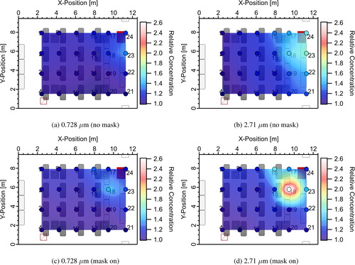
All results indicate some spatial non-uniformity in the aerosol distribution, even under steady-state conditions. This is not unexpected; obviously, at the exit of the manikin’s mouth the aerosol concentration will be maximum. As the jet of aerosol emitted from the manikin’s mouth entrains air and mixes the concentration will decrease. The level of non-uniformity appears to be a function of both the use of a mask and the size of the particles. The use of a mask clearly changes the penetration of aerosol in the direction that the jet exits the manikin’s mouth (towards the front of the classroom → increasing x-position). Without a mask, higher concentrations are seen further from the manikin location in the x-direction in Figure 7. The use of a mask, appears to localize the high concentration region closer to the emitting manikin. As will be shown later, the filtration provided by the mask also reduces overall aerosol concentrations.

Dependence of the distributions on particle size is also seen in Figure 7. The magnitude of non-uniformity appears to be smaller for the smaller particle size (0.728 μm). This may be explained by a higher loss rate due to settling for larger particles (Riley et al. 2002) resulting in lower concentrations of large particles farther from the source. The higher loss rate increases the peak relative concentration for larger particles since the distributions are normalized by the smallest concentration in the room for each case and diameter. This implies that smaller particle sizes are more uniformly distributed in the room and that the well-mixed assumption holds better for these particles.

One of the weaknesses of the current measurements is the coarse x–y resolution and lack of vertical resolution. The net result of this is that some sampling bias exists in the data. This is seen for the measurements at sample point 18 taken almost directly in front of the emitting manikin. In the no mask case, measurements taken directly in the center of the jet issuing from the manikin’s mouth should have the highest relative concentration of any measurements in the room and should have a higher relative concentration than the measurements at the same location for the mask on case. This is not seen in the relative concentration distributions in Figure 7 indicating sampling bias close to the source location. This may be due in part to vertical stratification, since measurements were made only at one height for a given x–y location. As one moves further from the source location, stratification becomes smaller, and the sampling bias should be a smaller effect. The relatively modest non-uniformity in concentrations measured over the majority of the room indicates that the well-mixed assumption in the Wells–Riley model should result in only modest errors in the infection probabilities for the reduced occupant densities studied; the uncertainty this introduces should be similar or smaller in magnitude than the uncertainty in other model input parameters such as the quanta emission rate.

3.2. Mask EFE

Size-resolved inhalation EFEs for the four masks tested (knit cotton mask, EOC mask, procedure mask, and surgical mask) are shown in Figure 8 for the three different cases tested: without a fitter, with the Badger Seal mask fitter, and with the FTM mask fitter. Total EFEs are shown in Figure 9 and the values are provided in Table 1. Overall, the results indicate that use of mask fitters can significantly improve the observed EFE. The observed EFEs with the mask fitters are believed to be similar to the MFEs of the masks, allowing comparison to previous work on mask material filtration efficiencies. The data for the size-resolved filtration efficiencies are provided in tables in the Supplemental Information. Also, data taken on material filtration efficiencies for the masks for a size range from 20 to 500 nm at a filtration velocity of 3.4 cm/s are provided in the Supplemental Information.

Fig. 8. Size-resolved effective filtration efficiency for inhalation measured in a classroom without a mask fitter used, with a Badger Seal mask fitter, and with a FTM mask brace installed for (a) the 4-ply knit cotton mask, (b) the EOC 3-ply spunbond polypropylene mask, (c) a single-use procedure mask, and (d) an ASTM F2100 level-2 rated surgical mask.

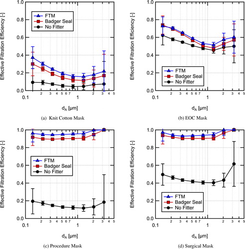
Fig. 9. Overall effective filtration efficiency for inhalation for the four masks tested in this work measured without a mask fitter, with the Badger Seal mask fitter, and the FTM mask brace used.

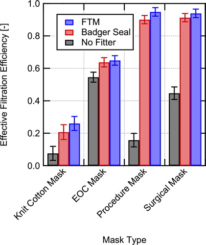
Table 1. Measured total effective filtration efficiencies and associated uncertainties during simulated inhalation for masks installed on a manikin in a classroom setting.

Abbrev.	Mask	Fitter	${\eta }_{f,M_{\mathit{inh}}}$	${\eta }_{f,M_{\mathit{inh}}}$ uncertainty	fL	fL uncertainty
KCM	Knit Cotton Mask	None	0.075	±0.043	0.710	±0.661
KCM-B	Knit Cotton Mask	Badger Seal	0.206	±0.045	–	–
KCM-F	Knit Cotton Mask	FTM	0.260	±0.043	–	–
EOCM	EOC Mask	None	0.545	±0.031	0.160	±0.084
EOCM-B	EOC Mask	Badger Seal	0.637	±0.029	–	–
EOCM-F	EOC Mask	FTM	0.649	±0.029	–	–
PM	Procedure Mask	None	0.158	±0.042	0.834	±0.053
PM-B	Procedure Mask	Badger Seal	0.900	±0.025	–	–
PM-F	Procedure Mask	FTM	0.949	±0.026	–	–
SM	Surgical Mask	None	0.447	±0.038	0.524	±0.050
SM-B	Surgical Mask	Badger Seal	0.913	±0.025	–	–
SM-F	Surgical Mask	FTM	0.939	±0.026	–	–

Estimated fraction of air leakage (f_L) and its associated uncertainty are also provided based on Equation 9(9) $$f_L=\frac{{\dot{V}}_{b,L}}{{\dot{V}}_b}=\frac{(1-{\eta }_{f,M_{\mathit{Inh}}})-(1-{\eta }_{f,M,\mathit{fit}})}{(1-(1-{\eta }_{f,M,\mathit{fit}}))}$$(9) .

The 4-ply knit cotton cloth mask (Figure 8a) without a mask fitter has the lowest EFE of 7.5 ± 4.3%. With the use of a mask fitter the filtration efficiency is still relatively low (26.0 ± 4.3% with the FTM mask brace), but is significantly improved over the entire size range. The lowest filtration efficiency corresponding to the most penetrating particle size (MPPS) occurs around 1 μm with and without a mask fitter. Lindsley et al. (2021a) tested a similar knit cotton 3-layer mask (Hanes mask) and found a MFE of 18.8%, in good agreement with the current result with the FTM mask brace given that their mask had one less layer and that the face velocities were different between the two studies. For particle sizes >3.2 μm, the filtration efficiency of the mask is anticipated to increase due to increasing efficiency of interception and impaction capture mechanisms (Hinds 1999), potentially providing effective filtration of particles >10 μm in diameter.

MFE is a function of the face velocity. Here, low to moderate breathing rates were simulated, at higher face velocities the MFE at larger particle sizes will increase due to the velocity dependence of the impaction capture mechanism, whereas filtration at small particles sizes will decrease due to a reduction in diffusion capture. Therefore, for high velocities associated with coughing and sneezing the MFE for larger particle sizes >2 μm is expected to improve, as is seen in the work of Drewnick et al. (2021) where filtration efficiency was found to increase with increasing face velocity at a particle size of 2.5 μm for a range of materials.

The EOC mask, composed of three layers of spunbond polypropylene (Figure 8b), had much higher EFE than the knit cotton mask. Additionally, the mask fit and sealed around the manikin’s face well as evidenced by only a moderate EFE increase when using either of the mask fitters. The overall EFE without a mask fitter was 54.5 ± 3.1% and was 64.9 ± 2.9% with the FTM mask brace for the aerosol distribution used here. The apparent MFE from the mask brace measurements per a layer (assuming typical exponential dependence of penetration on thickness (Hinds 1999)) is in reasonable agreement with data from Joo et al. (2021) for spunbond materials given differences in face velocity and other parameters for the measurements. As with the knit cotton mask, EFE is expected to continue to increase for larger particle sizes due to increased interception and impaction capture.

Of all the EFE results, those for the single-use procedure mask demonstrate the importance of mask fit the best. Without a mask fitter, the size-resolved efficiency is <20% for the entire range measured. With a mask fitter, the size-resolved EFE is generally greater than 90% with either mask fitter and is approximately 95% with the FTM mask brace. Measurements were also performed with the procedure mask with and without a Badger Seal mask fitter using a fit tester (TSI PortaCount Pro + 8038), those results showed similar trends (fit test results are provided in the Supplemental Information). The low overall EFE of 15.8 ± 4.2%, shown in Figure 9, for the single-use procedure mask was due to the poor natural fit of the mask when not using a mask fitter (as illustrated in the visualization provided in the Supplemental Information). Using a fitter enables the mask to achieve EFEs close to the MFE, which is approaching 100% for large particle sizes (>2 μm) at the face velocities used in the current testing. The apparent MFE for the mask with the fitters is high, but other studies have seen similar high MFEs for disposable masks, for example, Crilley et al. (2021) measured MFEs of 95.4 ± 1.9% and 84.3 ± 6.1% for two different disposable masks over the size range tested at a face velocity of 3 cm/s.

The surgical mask results demonstrate that the higher quality surgical mask provides better fit to the user’s face than the inexpensive single-use procedure mask (see Supplemental Information for images of the masks installed on the manikins). However, even with the better fit, the surgical mask without a fitter significantly under performs relative to the same mask worn with a fitter. Without a fitter the overall EFE was 44.6 ± 3.8% as compared to 91.3 ± 2.5% with the Badger Seal fitter and 93.9 ± 2.6% with the FTM mask brace. Given that the surgical mask was an ASTM F2100 level-2 rated mask, it should have MFE > 98% at 0.1 μm (ASTM 2019), which is in good agreement with the size-resolved apparent MFE based on the measurements with the FTM mask brace in Figure 8.

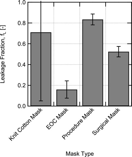
The measured filtration efficiencies with and without the mask fitters can be used to estimate the fraction of the flow leaking around a mask by making the following assumptions: (1) MFE does not change appreciably due to the difference in flow rate through the mask material and (2) the FTM mask brace case seals the mask perfectly, that is, there was no leakage for this case. Both assumptions will tend to underestimate the leakage rate. Using the filtration efficiencies for the cases with and without leakage, the fraction of flow leaking around the mask (fraction of air not going through the mask material) is estimated as (9) $$f_L=\frac{{\dot{V}}_{b,L}}{{\dot{V}}_b}=\frac{(1-{\eta }_{f,M_{\mathit{Inh}}})-(1-{\eta }_{f,M,\mathit{fit}})}{(1-(1-{\eta }_{f,M,\mathit{fit}}))}$$(9) where f_L is the fraction of flow leaking around the mask, ${\dot{V}}_{b,L}$ is the leakage volumetric flowrate, ${\eta }_{f,M_{\mathit{Inh}}}$ is the EFE with leakage present, and ${\eta }_{f,M,\mathit{fit}}$ is the MFE assumed to be equal to the filtration efficiency when using the FTM mask fitter.

Estimated leakage fractions for the cases with no mask fitters are shown in Figure 10. For the poorly fitting knit cotton mask and procedure mask, the leakage around the masks is estimated to be on the order of 70–85%, although the estimate for the knit cotton mask is highly uncertain due to the low filtration efficiency of the mask. The surgical mask which visually fits much better, still has an estimated leakage of 52%. Finally, the EOC mask which fit quite well has considerably less leakage at around 15%. These estimates emphasize the difficulty in achieving good mask fit without design features or additional devices to seal masks.

Fig. 10. Estimated fraction of flow that leaks around the masks without use of a mask fitter, calculated using Equation 9(9) $$f_L=\frac{{\dot{V}}_{b,L}}{{\dot{V}}_b}=\frac{(1-{\eta }_{f,M_{\mathit{Inh}}})-(1-{\eta }_{f,M,\mathit{fit}})}{(1-(1-{\eta }_{f,M,\mathit{fit}}))}$$(9) .

Other recent work has also shown the importance of mask fit on the EFE achieved with a mask. Clapp et al. (2021) found a significant increase in EFE from 38.5 ± 22.4% to 78.2 ± 6.6% for a medical procedure mask when using a rubber-band based mask fitter and up to 80.2 ± 6.2% for a nylon hosiery sleeve placed over the mask (measured using a fit tester). Significant improvements in EFEs were also seen by Mueller et al. (2020) when using a nylon hosiery sleeve to improve mask fit (measurements performed with a fit tester). The improvements in mask fit when using devices to actively seal the mask to the user’s face are similar to the improvement seen for all masks in the current study, although the methods of evaluation between those studies and the present study are quite different.

The EFEs for each of the mask options were only moderately sensitive to particle size for the range of sizes tested. Therefore, use of the overall EFEs is reasonable for the Wells–Riley model. Conditions measured represent an inhalation condition with steady flow, which ignores the unsteadiness of real breathing and does not directly measure exhalation EFE. However, we expect that the differences in filtration efficiency this causes will be moderate. Measurements of room aerosol concentration versus time for a case with a manikin exhaling and wearing the procedure mask with a Badger seal mask fitter were acquired and the results indicate similar EFE for exhalation as for inhalation in that specific case (see Supplemental Information for more details). Additionally, the results of Pan et al. (2021) indicate reasonably similar EFEs for inhalation and exhalation for a range of mask types.

4. Wells–Riley model results and discussion

The purpose of studying the aerosol dynamics and distribution in the classroom and the mask effective filtration efficiencies was to determine the accuracy of underlying model approximations and determine accurate input values for the Wells–Riley model. This allows increased confidence, that is, reduced uncertainty, in the model’s ability to estimate conditional infection probability.

4.1. Model input parameters and assumptions

Aerosol distribution results verified that the well-mixed approximation is reasonably accurate (to within better than a factor of 2) when individuals are physically distanced by >2 m. Aerosol dynamics results provided a direct measurement of the particle loss rate due to settling and HVAC system losses. Finally, the mask EFE measurements provide validated inputs for EFE with and without a mask fitter for the four masks tested.

With the aerosol behavior and EFE characterized, these results were used as inputs to the Wells–Riley model to assess the conditional infection probability in the event that one of the classroom’s occupants was COVID-19 positive and actively shedding the SARS-CoV-2 virus. We evaluate conditional infection probability for the following three scenarios: (a) Infectious instructor (speaking loudly), susceptible students (sedentary); (b) Infectious student (speaking), susceptible students; and (c) Infectious student (speaking), susceptible instructor (light exercise).

Given the differences in expiratory activity and activity level, different values of quanta emission rate and breathing rate are used for the instructor and students. Values used are provided in Table 2. The breathing rate for the students was chosen to correspond approximately to those from Adams (1993) for sitting or standing adults which closely match the flow rate used in the mask EFE testing. The value used for the instructor corresponds approximately to the breathing rate for walking adults from Adams (1993) (similar values were used in Buonanno, Morawska, and Stabile 2020a). The quanta emission rate, $\dot{q},$ is higher for the instructor who is assumed to be speaking loudly and frequently, compared to the students who are assumed to be seated and speaking less frequently. Values were determined using the emission rate distributions provided by Buonanno, Morawska, and Stabile (2020a) for light activity, speaking loudly, and for light activity, speaking, for the instructor and students, respectively, and then determining the approximate value of emission rate which has an infection probability that is equal to the risk defined by (10) $$R={\int }_0^{\infty }P(\dot{q})f(\dot{q})\mathrm{d}\dot{q}$$(10) where R is the risk of infection, $P(\dot{q})$ is the quanta emission rate dependent infection probability, and $f(\dot{q})$ is the probability density function for the quanta emission rate (more details on $f(\dot{q})d\dot{q}$ are given in the Supplemental Information). The risk of infection takes into account the distribution of potential emission rates for an infected individual (Buonanno, Morawska, and Stabile 2020a), whereas the infection probability does not. For both emission rates, the values correspond approximately to the 77 percentile of the emission rate distribution, making them representative of a high emission rate scenario.

Table 2. Scenarios used for the infection probability calculations.

	Scenario A	Scenario B	Scenario C
Setting	Classroom	Classroom	Classroom
Infected individual	Instructor	Student	Student
Emission rate, $\dot{q}$	110 quanta/h	19.1 quanta/h	19.1 quanta/h
Susceptible individual(s)	Students	Instructor	Students
Susceptible breathing rate, ${\dot{V}}_b$	0.540 m^3/h	1.38 m^3/h	0.540 m^3/h

The number of new infections expected for a given event can be predicted by multiplying the risk of infection (condition probability of infection) by the number of susceptible individuals present (11) $$N_{\mathit{event}}=R{N}_S.$$(11) The number of susceptible individuals (where N_S) is given by (12) $$N_S=(N_{\mathit{tot}}-N_I)(1-f_V{\eta }_V)$$(12) where N_tot is the total number of people present, N_I is the number of infected individuals present, f_V is the fraction of susceptibles who are vaccinated (local vaccination rate), and η_V is the efficacy of the vaccine for the preventing infection for the vaccinated individuals. This allows for direct accounting of vaccination rate and vaccine efficacy.

The room used for probability calculations for all three scenarios was the same classroom used for aerosol dynamics and spatial distribution measurements. The details of the room are provided in Table 3 along with values for the other remaining parameters needed for the calculations. To simplify the estimates, and due to lack of complete information on the filtration capabilities of the air handling unit (with MERV 15 filtration), it was assumed that all air supplied to the room is fresh air (i.e. quanta free), which will tend to slightly underestimate infection probability. For simplicity, it is also assumed that time between class periods in the room is long such that the initial concentration of quanta in the room is zero. Finally, it is assumed that the mask filtration efficiencies for inhalation and exhalation are equal.

Table 3. Parameter values for Wells–Riley conditional infection probability estimates.

Parameter	Description	Value	Units	Fixed/variable	Source
$V_R$	Room volume	362.64	m${}^3$	Fixed	Facility info.
$N_{\mathit{ACH}}$	Air changes per hour	1.34	h${}^{-1}$	Variable	Current study
${\lambda }_s$	Particle settling loss rate	0.35	h${}^{-1}$	Fixed	Current study
$k$	Virus inactivation rate	0.63	h${}^{-1}$	Fixed	(van Doremalen et al. 2020)
$\lambda$	Total loss rate (baseline)	2.32	h${}^{-1}$	Variable	$\lambda =N_{\mathit{ACH}}+k+{\lambda }_s$
$t_D$	Duration	60	min	Fixed	50 min class period + 10 min before/after
${\eta }_{f,M}$	Mask EFE	0	–	Variable	Baseline = 0 (no masks), for others see Table 1

For parameters that are varied in the calculations (variable) parameter values shown are the baseline values used or determined in the current study.

4.2. Model results with varying mask EFE and ventilation rate

The conditional probability of infection was predicted (under the condition of one infectious individual being present) for the three scenarios in Table 2 as a function of mask EFE with the baseline air-exchange rate, N_ACH = 1.34 h⁻¹ (assuming that everyone in the room is wearing the same type of mask), and as a function of ACH for the case with no one wearing masks, the results for both cases are shown in Figure 11. Of the three different scenarios studied, Scenario A, the case with an infected instructor and susceptible students, results in the highest conditional probability due to the assumed higher quanta emission rate for the instructor. Scenario B with an infected student and susceptible instructor had intermediate probability, and Scenario C with an infected student and susceptible students has the lowest probability, due to the lower quanta emission rate combined with the lower breathing rate.

Fig. 11. Estimated conditional probability of infection for aerosol transmission in a classroom for different intervention scenarios for (a) varying mask filtration efficiency (${\eta }_{f,M}$) and (b) varying number of air changes per hour (N_ACH).

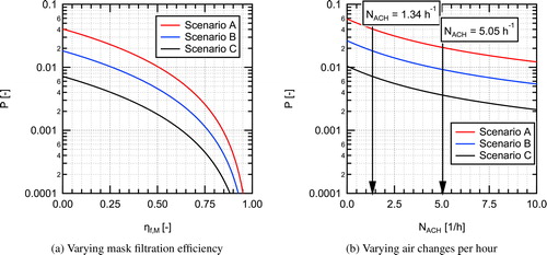
The spacing between curves for the three scenarios shown in Figure 11a and b remains constant on the vertical log scale as the parameter of interest is varied. This indicates a constant factor between the curves as a result of the differences in quanta emission rate and breathing rates for the three scenarios. As mask filtration efficiency is increased, the conditional infection probability decreases, somewhat slowly at first, then rapidly for higher mask EFEs. At a mask EFE of 0.5 (50%) the conditional infection probability is reduced by a factor of four relative to the baseline case with no masks (N_ACH = 1.34 h⁻¹). With everyone wearing a mask with an EFE of 0.9 (90%), the conditional infection probability is reduced by a factor of 100. This is due to the 10× decrease in quanta emitted to the room combine with the 10× decrease in quanta inhaled through a mask, resulting in a total reduction of a factor of 100 as one would anticipate from Equation 7(7) $$P\approx \frac{N_I\dot{q}}{\lambda V_R}{\dot{V}}_b{t}_D(1-{\eta }_{f,M_{\mathit{Inh}}})(1-{\eta }_{f,M_{\mathit{Exh}}}).$$(7) , greatly reducing the infection probability relative to the baseline value.

For the scenarios as a function of varying ACH (Figure 11b), the curves decrease faster at low values of N_ACH and conditional probability decreases slower with increasing N_ACH at higher values, indicating a diminishing return for increasing ventilation rates. The horizontal axis in Figure 11b can also be interpreted as total loss rate (λ) by increasing the values listed on the axis by ${\lambda }_s+k=0.98.$ Increasing from the baseline value of N_ACH=1.34 h⁻¹ to 5.05 h⁻¹ results in a decrease in infection probability by about a factor of two. Further increasing the air change rate to 10 h⁻¹ results in an additional factor of 1.7 decrease in infection probability. It is interesting to note that even at an air change rate of 10 h⁻¹ the infection probability for Scenario A cannot be reduced below 0.01 or 1%, whereas with everyone wearing the EOC mask without a fitter with the baseline air exchange in the room (N_ACH = 1.34), the probability of infection can be reduced to <0.009 (<0.9%). A heat map showing impacts of simultaneous variation of both mask EFE and ACH on the conditional infection probability is provided in the Supplemental Information.

4.3. Results for specific interventions

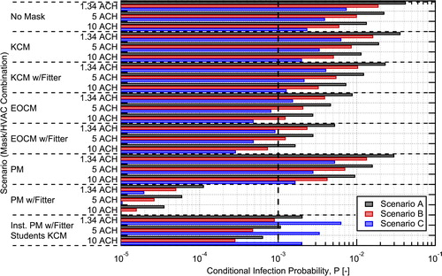
Conditional infection probabilities for the three scenarios in Table 2 were also estimated for specific combinations of HVAC flowrate (ACH), masks worn by students and an instructor, and the use of mask fitters. Three values of HVAC flowrate were used: 1.34 ACH (Baseline), 5 ACH, and 10 ACH. The use of an in-room recirculating air purifier could be considered as part of the HVAC flowrate in these calculations assuming 100% filtration efficiency for the purifier and no impact on the well-mixed model approximation. Calculations were performed for cases with everyone in the room wearing knit cotton masks (KCM), the EOC mask (EOCM), and the inexpensive procedure mask (PM), both with and without use of mask fitters (filtration values used are those for the masks with the FTM fitter). The surgical mask was not considered here due to higher cost, low availability, and the desire not to impact supplies for medical professionals, but performance would be similar to the EOCM without a fitter and almost identical to the procedure mask with a mask fitter. An additional case is also considered where the instructor is wearing a procedure mask with a mask fitter and the students are all wearing cloth masks. This case is focused on source control of the person who will likely have the highest quanta emission rate due to their known activity and who could be trained to consistently and properly don a mask and mask fitter. For each combination of interventions, conditional infection probabilities were calculated for the three scenarios in Table 2.

The conditional probability results for the different scenarios and intervention combinations are shown in Figure 12. Data for the conditional infection probabilities shown in the plot are provided in a table in the Supplemental Information. We have included a dashed line at a conditional probability of 0.001 on the plot for reference, this value was suggested in the recent publication of Buonanno, Morawska, and Stabile (2020a) as a target. The baseline case with no masks and 1.34 ACH has an estimated probability of infection of 0.042 (4.2%) for Scenario A, 0.0185 (1.85%) for Scenario B, and 0.0074 (0.74%) for Scenario C. For Scenario A considering the original room configuration with 48 students the number of estimated infections resulting from the event is $N_{\mathit{event}}=$ 2.0. For the reduced occupant density studied here, with only 16 students, this drops to $N_{\mathit{event}}=$ 0.67 infections, emphasizing the importance of reducing occupant density as a first step. It is interesting to note that for the configuration with 48 students a vaccination rate of 70.2% is required to achieve $N_{\mathit{event}}=$ 0.67, equivalent to the reduced occupant density case, when assuming a vaccine efficacy of 95%.

Fig. 12. Estimated conditional probability of infection for aerosol transmission in a classroom for different intervention combinations. A vertical dashed line is shown at the 0.001 conditional probability level. The mask abbreviations used on the graphs are: KCM = Knit Cotton Mask, EOCM = EOC Mask, PM = Procedure Mask.

The probabilities predicted here align well with those estimated in other works for conditional infection probabilities in similar classroom spaces when accounting for differences in exposure duration between the studies (Pavilonis et al. 2021; Shen et al. 2021; Stabile et al. 2021). For example, Pavilonis et al. (2021) found estimated mean conditional infection probabilites of 0.35 (35%) for the equivalent of Scenario A, with an exposure duration that was 6.3 times longer; accounting for the difference in exposure duration gives a result similar in magnitude to that found here. Shen et al. (2021) found a conditional infection probability of 3.1% for the equivalent of Scenario C for a 2 h exposure duration with 3.6 ACH, even correcting for exposure duration this is slightly higher than the value of 0.74% found here due to a higher quanta emission rate assumed in that study.

The addition of knit cotton masks for all classroom occupants yielded a modest 15% reduction in aerosol conditional infection probability compared to the baseline with no masks. In comparison, the protective measure of increasing the ventilation rate from 1.34 ACH to 5.0 ACH resulted in almost a factor of two (1.87×) reduction, regardless of mask worn. If a fitter is added to help seal the knit cotton mask to the user’s face, the conditional probability of infection is reduced by almost a factor of 2 (1.81×) relative to the no mask baseline. This reduction is similar to increasing the ventilation rate from 1.34 to 5.0 ACH, indicating that well fit cloth masks can play a significant role in reducing infection probability for aerosol transmission.

Combining higher ventilation rates with masks is synergistic and the impacts are multiplicative as indicated in Equation 7(7) $$P\approx \frac{N_I\dot{q}}{\lambda V_R}{\dot{V}}_b{t}_D(1-{\eta }_{f,M_{\mathit{Inh}}})(1-{\eta }_{f,M_{\mathit{Exh}}}).$$(7) . For example, the combination of knit cotton masks with mask fitters and an increase in ventilation rate from 1.34 to 5.0 ACH results in a factor of 3.4 reduction in conditional infection probability relative to the no mask baseline, which is equal to the product of the reductions for each individually. It is interesting to note that this combined reduction is greater than could be achieved by increasing HVAC flow from 1.34 to 10 ACH alone.

For masks with higher EFEs, we see more dramatic reductions in infection probability. For a moderate efficiency reusable mask like the EOC mask, factors of 4.75 and 8.2 reduction can be achieved without and with the use of a mask fitter, respectively. For the disposable procedure mask, the fit was poor without a mask fitter, it had only a 15.8% EFE, but with a mask fitter, an EFE of 94.8% could be achieved resulting in almost a factor of 400 reduction (371×) in conditional infection probability. This demonstrates the potential for reduction in aerosol transmission of SAR-CoV-2 achievable with relatively inexpensive masks and mask fitters.

The impact of ventilation rate found here is similar to that seen in other studies for indoor spaces like classrooms (Foster and Kinzel 2021; Stabile et al. 2021; Zhang 2020). On the other hand, other studies tend to over estimate the reduction in conditional infection probability for scenarios where masks are added (Shen et al. 2021; Zhang 2020), this is due to the lack of data in the literature on the influence of mask fit on EFE when these studies were published. For example, Shen et al. (2021) found that wearing cloth masks can reduce the conditional probability of infection by 48% on average, but only a 15% reduction for the knit cotton mask was found in the current work. A similar factor of two reduction in conditional infection probability was assumed by Zhang (2020). However, that level of reduction in conditional infection probability can likely only be achieved with typical cloth masks with the use of a mask fitter.

The case with the instructor using a procedure mask and mask fitter with the students using knit cotton masks, provides a look at how source control can provide significant reductions in infection probability and is attractive due to its cost effectiveness. In this case, by using a high efficiency mask on the person who is likely the highest emitter due to their known activity level, a reduction in the maximum conditional infection probability by a factor of 5.67 is achieved. Therefore, targeted interventions, where one or a few individuals are performing activities known to have high quanta emission rates, can have a large impact on infection probability. It also faces the reality that equipping and training an instructor on the proper donning of their mask is more readily achievable than relying on the same administrative control strategy for a larger number of student occupants.

The conditional infection probability results for the different interventions illustrate a few important points. First, increasing HVAC flowrate (ventilation), when possible, and ensuring a minimum acceptable ventilation rate, is important for reducing infection probability, but there is a decreasing return on investment (see Figure 11). Second, the three scenarios (from Table 2) result in significantly different probabilities due to the differences in emission rate and breathing rate between them. For the infectious instructor and susceptible students case (Scenario A), the conditional probability of infection is the highest due to the higher emission rate assumed for the lecturing instructor. For Scenario C, infectious student and susceptible students, the quanta emission rate is a factor of 5.76 lower (breathing rate is the same) and the conditional probability drops by a factor of 5.65, that is, approximately proportional with the reduction in quanta emission rate, as expected based on Equation 7(7) $$P\approx \frac{N_I\dot{q}}{\lambda V_R}{\dot{V}}_b{t}_D(1-{\eta }_{f,M_{\mathit{Inh}}})(1-{\eta }_{f,M_{\mathit{Exh}}}).$$(7) (the results shown here can easily be scaled to make estimates for different number of infectious individuals in the room, quanta emission rates, loss rates, room volumes, breathing rates, and mask filtration efficiencies). This suggests that source control, for cases where high quanta emission rates are likely, is a potentially effective strategy. Finally, it is clear that the use of masks and mask fitters, to reduce mask leakage (or better mask design to achieve the same result), can provide significant reductions in aerosol transmission infection probability, greater than those achievable by ventilation alone.

In the classroom space considered for this study, it is evident that ventilation rate alone will not be sufficient to achieve conditional infection probabilities below 0.001. Thankfully, as Equation 7(7) $$P\approx \frac{N_I\dot{q}}{\lambda V_R}{\dot{V}}_b{t}_D(1-{\eta }_{f,M_{\mathit{Inh}}})(1-{\eta }_{f,M_{\mathit{Exh}}}).$$(7) and the results illustrate, the combined effects of masks and ventilation are synergistic (multiplicative) and use of both simultaneously results in greater reductions in infection probability. For example, use of moderate filtration efficiency masks, like the EOC mask, along with elevated HVAC flowrates can come close to achieving 0.001 conditional infection probability in 2 out of the three scenarios (B and C). When considering return to normal operations with the widespread distribution of vaccines, achieving similar reductions in disease transmission via vaccination, as have been achieved through a combination of reduced occupant density and mask wearing in conventionally high-occupant density spaces like classrooms, will require high vaccination rates (>70%) and high vaccine efficacy.

5. Summary and conclusions

In this work, we took the unique approach of experimentally evaluating required input parameters related to ventilation and mask filtration efficiency and experimentally assessing the accuracy of the well-mixed assumption for the Wells–Riley model in a classroom at the University of Wisconsin-Madison. The validated inputs were then used in the Wells–Riley model to estimate conditional infection probabilities for SARS-CoV-2 in the same classroom setting. The model results provide valuable information on the effectiveness of masks, mask fitters, and ventilation rate interventions, and combinations of these, to reduce aerosol conditional infection probability in classroom settings.

The major conclusions from this work are summarized here:

1. Particle loss rates estimated from ventilation rates match well with those determined from aerosol concentration time evolution.

2. Based on in situ measurements in a representative classroom with forced air mechanical ventilation, the well-mixed assumption holds to a reasonable approximation (within better than a factor of 2) for distances >2 m from the source for the classroom space studied.

3. Leakage rates around masks are typically in the range of 20–80% when fit reasonably well to the user’s face, resulting in EFEs that are much lower than the MFEs.

4. With mask fitters, EFE approaching the MFE for a mask can be achieved. Inexpensive disposable masks used with a mask fitter can achieve close to 95% EFE in some cases.

5. Ventilation of spaces with fresh air or well-filtered air is important, but ventilation rates greater than >5 ACH result in only modest additional reductions in infection probability and may not be merited due to their high cost and other factors.

6. With all occupants in the indoor classroom wearing masks, aerosol conditional infection probabilities are greatly reduced and reductions of 4×, 10×, or even 100× can be achieved.

7. Source control, that is, providing an individual performing a known high emission rate activity with a high EFE mask (with a mask fitter), can be an effective approach to limit aerosol transmission infection probabilities.

8. Use of masks and ventilation simultaneously are synergistic (providing multiplicative reductions) and together can provide greatly reduced aerosol transmission infection probability.

The results of the current work provide guidance on the relative effectiveness of ventilation, mask wearing, mask fitters, and combinations thereof for decreasing aerosol transmission infection probabilities. They specifically emphasize the large potential for effective mask wearing and improved masks, or use of mask fitters, to greatly reduce infection probabilities. The results also indicate that achieving COVID-19 transmission rates similar to those achieved with reduced occupant density, improved ventilation, and mask wearing, will require high vaccination rates ($>70\%$) and high vaccine efficacy when returning to pre-pandemic levels of occupancy in classrooms without additional measures (like masks) in place.

Author contributions

David Rothamer: Conceptualization (equal); Data curation (lead); Formal Analysis (lead); Investigation (lead); Methodology (lead); Project administration (lead); Resources (equal); Software (lead); Supervision (lead); Validation (lead); Visualization (lead); Writing – Original draft preparation (lead); Writing – review and editing (equal); Scott Sanders Conceptualization (equal); Investigation (supporting); Methodology (supporting); Project administration (supporting); Resources (equal); Supervision (supporting); Writing – review and editing (equal); Tim Bertram: Conceptualization (supporting); Investigation (supporting); Methodology (supporting); Writing – review and editing (equal); Douglas Reindl: Conceptualization (supporting); Investigation (supporting); Methodology (supporting); Writing – Original draft preparation (supporting); Writing – review and editing (equal).

Acknowledgments

The authors would like to acknowledge the useful inputs and assistance from James Morrsion, Jesse Decker, Jessica Cebula, and Christopher Strang, and others in Environment, Health & Safety, the College of Engineering, and Facilities Planning and Management at the University of Wisconsin-Madison. The authors would like to also acknowledge Lennon Rodgers and employees of the University of Wisconsin-Madison Makerspace for their efforts on the design and manufacturing of the Badger Seal mask fitter which was inspired in part by the initial portions of this work. The authors would also like to thank graduates students Logan Kossel and James Rice as well as Prof. Alejandro Roldn-Alzate for their useful inputs and assistance.

Conflict of interest

The authors of this paper certify that they have no affiliations with or involvement in any organization or entity with any financial or non-financial interest in the subject matter or materials discussed in this manuscript.

Data availability statement

Data that support the findings of this study are available from the corresponding author upon reasonable request.

References

- 42 CFR Part 84. 2021. Code of federal regulations.
- Adams, W. C. 1993. Measurement of breathing rate and volume in routinely performed daily activities. Report, Physical Education Department, University of California, Davis, Human Performance Laboratory.
- Alsved, M., A. Matamis, R. Bohlin, M. Richter, P. E. Bengtsson, C. J. Fraenkel, P. Medstrand, and J. Löndahl. 2020. Exhaled respiratory particles during singing and talking. Aerosol Science and Technology 54 (11):1245–8. doi:https://doi.org/10.1080/02786826.2020.1812502
- ASTM. 2019. ASTM F2100-19E1: Standard specification for performance of materials used in medical face masks.
- Azimi, P., and B. Stephens. 2013. Hvac filtration for controlling infectious airborne disease transmission in indoor environments: Predicting risk reductions and operational costs. Building and Environment 70:150–60. doi:https://doi.org/10.1016/j.buildenv.2013.08.025
- Bagheri, M. H., I. Khalaji, A. Azizi, R. T. Loibl, N. Basualdo, S. Manzo, M. L. Gorrepati, S. Mehendale, C. Mohr, and S. N. Schiffres. 2021. Filtration efficiency, breathability, and reusability of improvised materials for face masks. Aerosol Science and Technology 1–15.
- Brooks, J. T., D. H. Beezhold, J. D. Noti, J. P. Coyle, R. C. Derk, F. M. Blachere, and W. G. Lindsley. 2021. Maximizing fit for cloth and medical procedure masks to improve performance and reduce sars-cov-2 transmission and exposure, 2021. Morbidity and Mortality Weekly Report 70 (7):254–7. doi:https://doi.org/10.15585/mmwr.mm7007e1
- Buonanno, G., L. Morawska, and L. Stabile. 2020a. Quantitative assessment of the risk of airborne transmission of SARS-CoV-2 infection: Prospective and retrospective applications. Environment International 145:106112. doi:https://doi.org/10.1016/j.envint.2020.106112
- Buonanno, G., L. Stabile, and L. Morawska. 2020b. Estimation of airborne viral emission: Quanta emission rate of SARS-CoV-2 for infection risk assessment. Environment International 141:105794. doi:https://doi.org/10.1016/j.envint.2020.105794
- CDC, U. S. 2020a. Scientific brief: Community use of cloth masks to control the spread of SARS-CoV-2. Report, Centers for Disease Control and Prevention.
- CDC, U. S. 2020b. Scientific brief: SARS-CoV-2 and potential airborne transmission. 2020. Report, Centers for Disease Control and Prevention.
- Chia, P. Y., K. K. Coleman, Y. K. Tan, S. W. X. Ong, M. Gum, S. K. Lau, X. F. Lim, A. S. Lim, S. Sutjipto, P. H. Lee, et al. 2020. Detection of air and surface contamination by SARS-CoV-2 in hospital rooms of infected patients. Nature Communications 11 (1):2800. doi:https://doi.org/10.1038/s41467-020-16670-2
- Clapp, P. W., E. E. Sickbert-Bennett, J. M. Samet, J. Berntsen, K. L. Zeman, D. J. Anderson, D. J. Weber, and W. D. Bennett. 2021 Evaluation of cloth masks and modified procedure masks as personal protective equipment for the public during the covid-19 pandemic. JAMA Internal Medicine 181 (4):463–9. doi:https://doi.org/10.1001/jamainternmed.2020.8168
- Clase, C. M., E. L. Fu, A. Ashur, R. C. L. Beale, I. A. Clase, M. B. Dolovich, M. J. Jardine, M. Joseph, G. Kansiime, J. F. E. Mann, et al. 2020. Forgotten technology in the COVID-19 pandemic: Filtration properties of cloth and cloth masks – A narrative review. Mayo Clinic Proceedings 95 (10):2204–24. doi:https://doi.org/10.1016/j.mayocp.2020.07.020
- Crilley, L. R., A. A. Angelucci, B. Malile, C. J. Young, T. C. VandenBoer, and J. I. L. Chen. 2021. Non-woven materials for cloth-based face masks inserts: Relationship between material properties and sub-micron aerosol filtration. Environmental Science: Nano.
- Davies, A., K.-A. Thompson, K. Giri, G. Kafatos, J. Walker, and A. Bennett. 2013. Testing the efficacy of homemade masks: Would they protect in an influenza pandemic? Disaster Medicine and Public Health Preparedness 7 (4):413–8. doi:https://doi.org/10.1017/dmp.2013.43
- Drewnick, F., J. Pikmann, F. Fachinger, L. Moormann, F. Sprang, and S. Borrmann. 2021. Aerosol filtration efficiency of household materials for homemade face masks: Influence of material properties, particle size, particle electrical charge, face velocity, and leaks. Aerosol Science and Technology 55 (1):63–79. doi:https://doi.org/10.1080/02786826.2020.1817846
- Fennelly, K. P. 2020. Particle sizes of infectious aerosols: Implications for infection control. The Lancet Respiratory Medicine 8 (9):914–24. doi:https://doi.org/10.1016/S2213-2600(20)30323-4
- Fennelly, K. P., and E. A. Nardell. 1998. The relative efficacy of respirators and room ventilation in preventing occupational tuberculosis. Infection Control and Hospital Epidemiology 19 (10):754–9. doi:https://doi.org/10.2307/30141420
- Fisk, W. J., O. Seppänen, D. Faulkner, and J. Huang. 2005. Economic benefits of an economizer system: Energy savings and reduced sick leave. In ASHRAE Transactions, vol. 111, PART 2, 673–9.
- Foster, A., and M. Kinzel. 2021. Estimating covid-19 exposure in a classroom setting: A comparison between mathematical and numerical models. Physics of Fluids (Woodbury, N.Y.: 1994) 33 (2):021904. doi:https://doi.org/10.1063/5.0040755
- Gammaitoni, L., and M. C. Nucci. 1997. Using a mathematical model to evaluate the efficacy of tb control measures. Emerging Infectious Diseases 3 (3):335–42. doi:https://doi.org/10.3201/eid0303.970310
- Hao, W., A. Parasch, S. Williams, J. Li, H. Ma, J. Burken, and Y. Wang. 2020. Filtration performances of non-medical materials as candidates for manufacturing facemasks and respirators. International Journal of Hygiene and Environmental Health 229:113582. doi:https://doi.org/10.1016/j.ijheh.2020.113582
- Hao, W., G. Xu, and Y. Wang. 2021. Factors influencing the filtration performance of homemade face masks. Journal of Occupational and Environmental Hygiene 18 (3):128–38. doi:https://doi.org/10.1080/15459624.2020.1868482
- Hendrix, M. J., C. Walde, K. Findley, and R. Trotman. 2020. Absence of apparent transmission of SARS-CoV-2 from two stylists after exposure at a hair salon with a universal face covering policy—Springfield, Missouri, May 2020. Morbidity and Mortality Weekly Report 69 (28):930–2. doi:https://doi.org/10.15585/mmwr.mm6928e2
- Hill, W. C., M. S. Hull, and R. I. MacCuspie. 2020. Testing of commercial masks and respirators and cotton mask insert materials using SARS-CoV-2 virion-sized particulates: Comparison of ideal aerosol filtration efficiency versus fitted filtration efficiency. Nano Letters 20 (10):7642–7. doi:https://doi.org/10.1021/acs.nanolett.0c03182
- Hinds, W. C. 1999. Aerosol Technology: Properties, Behavior, and Measurement of Airborne Particles. New York: John Wiley & Sons, Inc.
- Holmgren, H., B. Bake, A.-C. Olin, and E. Ljungström. 2011. Relation between humidity and size of exhaled particles. Journal of Aerosol Medicine and Pulmonary Drug Delivery 24 (5):253–60. doi:https://doi.org/10.1089/jamp.2011.0880
- Jang Ji, Y., and W. Kim Seung. 2015. Comparative evaluation of filtration efficiency performance of similar mask products on the market. Journal of the Korean Society of Environmental Health 41 (3):203–15.
- Johnson, G. R., L. Morawska, Z. D. Ristovski, M. Hargreaves, K. Mengersen, C. Y. H. Chao, M. P. Wan, Y. Li, X. Xie, D. Katoshevski, et al. 2011. Modality of human expired aerosol size distributions. Journal of Aerosol Science 42 (12):839–51. doi:https://doi.org/10.1016/j.jaerosci.2011.07.009
- Joo, T., M. Takeuchi, F. Liu, M. P. Rivera, J. Barr, E. S. Blum, E. Parker, J. H. Tipton, J. Varnedoe, B. Dutta, et al. 2021. Evaluation of particle filtration efficiency of commercially available materials for homemade face mask usage. Aerosol Science and Technology, Pages 1–15.
- Jung, H., J. K. Kim, S. Lee, J. Lee, J. Kim, P. Tsai, and C. Yoon. 2014. Comparison of filtration efficiency and pressure drop in anti-yellow sand masks, quarantine masks, medical masks, general masks, and handkerchiefs. Aerosol and Air Quality Research 14 (3):991–1002. doi:https://doi.org/10.4209/aaqr.2013.06.0201
- Kelly, E., S. Pirog, J. Ward, and P. J. Clarkson. 2020. Ability of fabric face mask materials to filter ultrafine particles at coughing velocity. BMJ Open 10 (9):e039424. doi:https://doi.org/10.1136/bmjopen-2020-039424
- Kohanski, M. A., L. J. Lo, and M. S. Waring. 2020. Review of indoor aerosol generation, transport, and control in the context of COVID-19. International Forum of Allergy & Rhinology 10 (10):1173–9. doi:https://doi.org/10.1002/alr.22661
- Konda, A., A. Prakash, G. Moss, M. Schmoldt, G. Grant, and S. Guha. 2020a. Correction to aerosol filtration efficiency of common fabrics used in respiratory cloth masks. ACS Nano 14 (8):10742–3. doi:https://doi.org/10.1021/acsnano.0c04676
- Konda, A., A. Prakash, G. A. Moss, M. Schmoldt, G. D. Grant, and S. Guha. 2020b. Aerosol filtration efficiency of common fabrics used in respiratory cloth masks. ACS Nano 14 (5):6339–47. doi:https://doi.org/10.1021/acsnano.0c03252
- Lawrence, R. B., M. G. Duling, C. A. Calvert, and C. C. Coffey. 2006. Comparison of performance of three different types of respiratory protection devices. Journal of Occupational and Environmental Hygiene 3 (9):465–74. doi:https://doi.org/10.1080/15459620600829211
- Leung, N. H. L., D. K. W. Chu, E. Y. C. Shiu, K.-H. Chan, J. J. McDevitt, B. J. P. Hau, H.-L. Yen, Y. Li, D. K. M. Ip, J. S. M. Peiris, et al. 2020. Respiratory virus shedding in exhaled breath and efficacy of face masks. Nature Medicine 26 (5):676–80. doi:https://doi.org/10.1038/s41591-020-0843-2
- Lindsley, W. G., F. M. Blachere, D. H. Beezhold, B. F. Law, R. C. Derk, J. M. Hettick, K. Woodfork, W. T. Goldsmith, J. R. Harris, M. G. Duling, et al. 2021a. A comparison of performance metrics for cloth face masks as source control devices for simulated cough and exhalation aerosols. medRxiv.
- Lindsley, W. G., F. M. Blachere, B. F. Law, D. H. Beezhold, and J. D. Noti. 2021b. Efficacy of face masks, neck gaiters and face shields for reducing the expulsion of simulated cough-generated aerosols. Aerosol Science and Technology 55 (4):449–57. doi:https://doi.org/10.1080/02786826.2020.1862409
- Long, K. D., E. V. Woodburn, I. C. Berg, V. Chen, and W. S. Scott. 2020. Measurement of filtration efficiencies of healthcare and consumer materials using modified respirator fit tester setup. PLOS One 15 (10):e0240499. doi:https://doi.org/10.1371/journal.pone.0240499
- Lu, J., J. Gu, K. Li, C. Xu, W. Su, Z. Lai, D. Zhou, C. Yu, B. Xu, and Z. Yang. 2020. COVID-19 outbreak associated with air conditioning in restaurant, Guangzhou, China, 2020. Emerging Infectious Diseases 26 (7):1628–31. doi:https://doi.org/10.3201/eid2607.200764
- Miller, S. L., W. W. Nazaroff, J. L. Jimenez, A. Boerstra, G. Buonanno, S. J. Dancer, J. Kurnitski, L. C. Marr, L. Morawska, and C. Noakes. 2020. Transmission of SARS-CoV-2 by inhalation of respiratory aerosol in the Skagit Valley Chorale superspreading event. Indoor Air.
- Morawska, L. 2006. Droplet fate in indoor environments, or can we prevent the spread of infection? Indoor Air 16 (5):335–47. doi:https://doi.org/10.1111/j.1600-0668.2006.00432.x
- Morawska, L., J. Allen, W. Bahnfleth, P. M. Bluyssen, A. Boerstra, G. Buonanno, J. Cao, S. J. Dancer, A. Floto, F. Franchimon, et al. 2021. A paradigm shift to combat indoor respiratory infection. Science (New York, N.Y.) 372 (6543):689–91. doi:https://doi.org/10.1126/science.abg2025
- Morawska, L., and J. Cao. 2020. Airborne transmission of SARS-CoV-2: The world should face the reality. Environment International 139:105730. doi:https://doi.org/10.1016/j.envint.2020.105730
- Morawska, L., G. R. Johnson, Z. D. Ristovski, M. Hargreaves, K. Mengersen, S. Corbett, C. Y. H. Chao, Y. Li, and D. Katoshevski. 2009. Size distribution and sites of origin of droplets expelled from the human respiratory tract during expiratory activities. Journal of Aerosol Science 40 (3):256–69. doi:https://doi.org/10.1016/j.jaerosci.2008.11.002
- Morawska, L., and D. K. Milton. 2020. It is time to address airborne transmission of COVID-19. Clinical Infectious Diseases. doi:https://doi.org/10.1093/cid/ciaa939
- Mueller, A. V., M. J. Eden, J. M. Oakes, C. Bellini, and L. A. Fernandez. 2020. Quantitative method for comparative assessment of particle removal efficiency of fabric masks as alternatives to standard surgical masks for PPE. Matter 3 (3):950–62. doi:https://doi.org/10.1016/j.matt.2020.07.006
- Nardell, E. A., and R. R. Nathavitharana. 2020. Airborne spread of SARS-CoV-2 and a potential role for air disinfection. JAMA 324 (2):141–2. doi:https://doi.org/10.1001/jama.2020.7603
- Nazaroff, W. 2004. Indoor particle dynamics. Indoor Air 14 (s7):175–83. doi:https://doi.org/10.1111/j.1600-0668.2004.00286.x
- Nazaroff, W. W., M. Nicas, and S. L. Miller. 1998. Framework for evaluating measures to control nosocomial tuberculosis transmission. Indoor Air 8 (4):205–18. doi:https://doi.org/10.1111/j.1600-0668.1998.00002.x
- Nicas, M., W. W. Nazaroff, and A. Hubbard. 2005. Toward understanding the risk of secondary airborne infection: Emission of respirable pathogens. Journal of Occupational and Environmental Hygiene 2 (3):143–54. doi:https://doi.org/10.1080/15459620590918466
- NIOSH. 2019. Determination of particulate filter efficiency level for n95 series filters against solid particulates for non-powered, air-purifying respirators standard test procedure (stp).
- Nissen, K., J. Krambrich, D. Akaberi, T. Hoffman, J. Ling, Å. Lundkvist, L. Svensson, and E. Salaneck. 2020. Long-distance airborne dispersal of SARS-CoV-2 in COVID-19 wards. Scientific Reports 10 (1):19589. doi:https://doi.org/10.1038/s41598-020-76442-2
- Noakes, C. J., and P. A. Sleigh. 2009. Mathematical models for assessing the role of airflow on the risk of airborne infection in hospital wards. Journal of the Royal Society, Interface 6 (Suppl 6):S791–S800.
- Pan, J., C. Harb, W. Leng, and L. C. Marr. 2021. Inward and outward effectiveness of cloth masks, a surgical mask, and a face shield. Aerosol Science and Technology 55 (6):718–33. doi:https://doi.org/10.1080/02786826.2021.1890687
- Pavilonis, B., A. M. Ierardi, L. Levine, F. Mirer, and E. A. Kelvin. 2021. Estimating aerosol transmission risk of SARS-CoV-2 in New York City public schools during reopening. Environmental Research 195:110805. doi:https://doi.org/10.1016/j.envres.2021.110805
- Rengasamy, S., B. Eimer, and R. E. Shaffer. 2010. Simple respiratory protection–evaluation of the filtration performance of cloth masks and common fabric materials against 20–1000 nm size particles. The Annals of Occupational Hygiene 54 (7):789–98. doi:https://doi.org/10.1093/annhyg/meq044
- Riley, E., G. Murphy, and R. Riley. 1978. Airborne spread of measles in a suburban elementary school. American Journal of Epidemiology 107 (5):421–32. doi:https://doi.org/10.1093/oxfordjournals.aje.a112560
- Riley, W. J., T. E. McKone, A. C. K. Lai, and W. W. Nazaroff. 2002. Indoor particulate matter of outdoor origin: Importance of size-dependent removal mechanisms. Environmental Science & Technology 36 (2):200–7. doi:https://doi.org/10.1021/es010723y
- Shen, J., M. Kong, B. Dong, M. J. Birnkrant, and J. Zhang. 2021. A systematic approach to estimating the effectiveness of multi-scale IAQ strategies for reducing the risk of airborne infection of SARS-CoV-2. Building and Environment 200:107926. doi:https://doi.org/10.1016/j.buildenv.2021.107926
- Smith, S. H., G. A. Somsen, C. v Rijn, S. Kooij, L. v d Hoek, R. A. Bem, and D. Bonn. 2020. Aerosol persistence in relation to possible transmission of SARS-CoV-2. Physics of Fluids (Woodbury, N.Y.: 1994) 32 (10):107108. doi:https://doi.org/10.1063/5.0027844
- Somsen, G. A., C. van Rijn, S. Kooij, R. A. Bem, and D. Bonn. 2020a. Measurement of small droplet aerosol concentrations in public spaces using handheld particle counters. medRxiv.
- Somsen, G. A., C. van Rijn, S. Kooij, R. A. Bem, and D. Bonn. 2020b. Small droplet aerosols in poorly ventilated spaces and SARS-CoV-2 transmission. The Lancet. Respiratory Medicine 8 (7):658–9. doi:https://doi.org/10.1016/S2213-2600(20)30245-9
- Stabile, L., A. Pacitto, A. Mikszewski, L. Morawska, and G. Buonanno. 2021. Ventilation procedures to minimize the airborne transmission of viruses at schools. medRxiv.
- Teesing, G. R., B. van Straten, P. de Man, and T. Horeman-Franse. 2020. Is there an adequate alternative to commercially manufactured face masks? a comparison of various materials and forms. Journal of Hospital Infection 106 (2):246–53. doi:https://doi.org/10.1016/j.jhin.2020.07.024
- Tham, K. W. 2016. Indoor air quality and its effects on humans—A review of challenges and developments in the last 30 years. Energy and Buildings 130:637–50. doi:https://doi.org/10.1016/j.enbuild.2016.08.071
- Ueki, H., Y. Furusawa, K. Iwatsuki-Horimoto, M. Imai, H. Kabata, H. Nishimura, and Y. Kawaoka. 2020. Effectiveness of face masks in preventing airborne transmission of SARS-CoV-2. mSphere 5 (5):e00637–20.
- van der Sande, M., P. Teunis, and R. Sabel. 2008. Professional and home-made face masks reduce exposure to respiratory infections among the general population. PLOS One 3 (7):e2618. doi:https://doi.org/10.1371/journal.pone.0002618
- Van Der Steen, J. M., M. G. Loomans, N. Schellens, and J. L. Hensen. 2017. Full-scale performance assessment of an innovative climate system for a classroom environment. In Healthy Buildings Europe 2017, HB 2017. International Society of Indoor Air Quality and Climate-ISIAQ, 1–6.
- van Doremalen, N., T. Bushmaker, D. H. Morris, M. G. Holbrook, A. Gamble, B. N. Williamson, A. Tamin, J. L. Harcourt, N. J. Thornburg, S. I. Gerber, et al. 2020. Aerosol and surface stability of SARS-CoV-2 as compared with SARS-CoV-1. The New England Journal of Medicine 382 (16):1564–7. doi:https://doi.org/10.1056/NEJMc2004973
- Wallace, L. 1996. Indoor particles: A review. Journal of the Air & Waste Management Association (1995) 46 (2):98–126. doi:https://doi.org/10.1080/10473289.1996.10467451
- Wang, Y., H. Tian, L. Zhang, M. Zhang, D. Guo, W. Wu, X. Zhang, G. L. Kan, L. Jia, D. Huo, et al. 2020. Reduction of secondary transmission of SARS-CoV-2 in households by face mask use, disinfection and social distancing: A cohort study in Beijing, China. BMJ Global Health 5 (5):e002794. doi:https://doi.org/10.1136/bmjgh-2020-002794
- Wells, W. 1955. Airborne Contagion and Air Hygiene. Cambridge, Mass.: Harvard University Press.
- Wells, W. F. 1955. Airborne contagion and air hygiene. An ecological study of droplet infections. Airborne Contagion and Air Hygiene. An Ecological Study of Droplet Infections.
- Whiley, H., T. P. Keerthirathne, M. A. Nisar, M. A. White, and K. E. Ross. 2020. Viral filtration efficiency of fabric masks compared with surgical and N95 masks. Pathogens 9 (9):762. doi:https://doi.org/10.3390/pathogens9090762
- WHO. 2020a. Coronavirus disease (covid-19) advice for the public: When and how to use masks.
- WHO. 2020b. Key planning recommendations for mass gatherings in the context of the current COVID-19 outbreak.
- WHO. 2020c. Recommendations to member states to improve hand hygiene practices to help prevent the transmission of the COVID-19 virus.
- Zhang, J. 2020. Integrating IAQ control strategies to reduce the risk of asymptomatic SARS Cov-2 infections in classrooms and open plan offices. Science and Technology for the Built Environment 26 (8):1013–8. doi:https://doi.org/10.1080/23744731.2020.1794499
- Zhao, M., L. Liao, W. Xiao, X. Yu, H. Wang, Q. Wang, Y. L. Lin, F. S. Kilinc-Balci, A. Price, L. Chu, et al. 2020. Household materials selection for homemade cloth face coverings and their filtration efficiency enhancement with triboelectric charging. Nano Letters 20 (7):5544–52. doi:https://doi.org/10.1021/acs.nanolett.0c02211
- Zhu, S., S. Kato, and J.-H. Yang. 2006. Study on transport characteristics of saliva droplets produced by coughing in a calm indoor environment. Building and Environment 41 (12):1691–702. doi:https://doi.org/10.1016/j.buildenv.2005.06.024