Algorithm for searching optimal set values of absorption chiller system using Bayesian optimization

Abstract

HVAC systems account for at least 40% of the energy consumption of general office buildings. Therefore, reducing the energy use of HVAC systems is indispensable. HVAC systems used in public office buildings mostly adopt a central air conditioning system. To save energy in the central air conditioning system, high-efficiency heat source machines have been adopted, and the inverter control of pumps has been generally introduced. As a further measure to save energy, an optimal control has been proposed. Model-based control has been mainly studied. However, the target HVAC system must be appropriately equipped with sensors for model-based control to use previous operation data. To solve this problem, we proposed a model-free optimal control method using Bayesian optimization. We verified its effectiveness in one-on-one (one cooling tower and one chiller) HVAC systems. As a result, the energy-saving ratio when compared to the rated specification control is 10.38% for our proposed method and 11.34% for the model-based approach, which shows the equivalent performance. In addition, the training results indicate that the optimal set values can be automatically determined in 4 weeks as the training proceeds under rated specification control with Bayesian optimization.

Introduction

The Paris Agreement has entered into force as a global measure against climate change. This agreement aims to hold the global average temperature increase below 2 °C above preindustrial levels and to pursue efforts to limit the temperature increase to 1.5 °C above preindustrial levels (United Nations 2015).

Japan’s target to reduce greenhouse gas emissions by 2030 is 26% compared to 2013 (MEGJ 2020). The “business and other sectors” such as general office buildings and commercial buildings and the residential sector with the largest reduction potential rate will be reduced by 40% by 2030. Furthermore, in April 2021the Japanese government announced its aim to raise the 2030 target to a 46% reduction, which may require further energy conservation (JG 2021). HVAC systems account for at least 40% of general office buildings’ energy consumption and CO₂ emission (ECCJ 2021).

HVAC systems used in general office buildings mostly adopt the central air conditioning system, in which chilled water and hot water are sent from the machine room and thermally exchanged with air by an air handling unit for heating and cooling. High-efficiency heat source machines have been adopted to save energy in the central air conditioning system, and the inverter control of pumps has been generally introduced. However, the state of buildings changes under climate and tenant conditions that were not assumed at the design stage. Therefore, energy saving of buildings should be tackled continuously in response to such changes. Optimal control (Braun and Diderrich 1990) can be used for HVAC systems to accommodate such changes. In optimal control, each unit and the entire HVAC system are operated under the highest energy efficiency in response to changes in ambient conditions and building loads. A comprehensive review of building HVAC’s optimal control is presented in Wang and Ma (2008).

The field of optimal control is roughly classified into model-based and model-free control. Model-based control, such as black-box and physical model-based controls, have been mainly studied.

Chow et al. (2002) proposed a black-box model-based optimal control for an absorption chiller system using a neural network and a genetic algorithm. Ignjatovic et al. (2016) developed a physical model-based control using the simulation tool EnergyPlus to minimize the primary energy consumption of an existing office building while maintaining the thermal comfort of its occupants.

Although model-based control has been studied extensively, it has some drawbacks. The parameters of model-based control are determined based on field test results conducted under different operating conditions and previous operation data. HVAC systems experts should set the operating conditions of field tests. The target HVAC system must be appropriately equipped with sensors to use the last operation data. These requirements may greatly affect the model’s accuracy.

For example, model-based control cannot be used when individual units are not equipped with watt-hour meters, and only the total power of a distribution board can be obtained. Therefore, in this study, we propose a model-free control method using Bayesian optimization to control a cooling water system to realize optimal control of HVAC systems that are not appropriately handled by the already-mentioned model-based control approaches.

Model-free control has broad applicability and high flexibility because it does not require a target system model or prior environment knowledge. Qiu et al. (2020) proposed a model-free control based on reinforcement learning (Sutton and Barto 1998) for the cooling water system of HVAC systems. Deng and Wang (2018) collected 1-year energy data from an office building and developed a prediction model for indoor temperature and humidity using Deep Neural Networks (Goodfellow, Bengio, and Courville 2016). By integrating their model with an energy optimization algorithm, they reduced energy consumption while maintaining thermal comfort. Kuroha et al. (2018) developed an algorithm for the automatic operation of HEMS air conditioners to improve the thermal environment and reduce electricity costs. They proposed a method that learns the characteristics of the equipment from past operation data and provides an air conditioner operation plan tailored to the installation environment. Telsang et al. (2019) adopted model-free control to regulate the indoor temperature using an HVAC system. They investigated the stability conditions of the control design under constrained inputs. Zhang et al. (2020) suggested a learning framework that leverages the Internet of Things (IoT) to automatically identify a thermal model for each thermal zone in a building. They used low-resolution temperature measurements from low-cost IoT devices to train the thermal model. Cui et al. (2021) proposed an air balancing method to achieve accurate air supply for satisfactory indoor air quality and better energy-saving performance.

Model-free control varies widely in terms of target systems and objectives. This study automates the energy conservation of the central air conditioning system installed in an office building. It is essential to keep the chilled water temperature constant to maintain indoor thermal comfort. The control of the indoor-side air conditioning system is to regulate the chilled water temperature and chilled water flow rate so that thermal comfort can be maintained under any condition of external factors such as heat load. Therefore, the thermal comfort of the room is guaranteed by setting a constraint to keep the chilled water temperature and chilled water flow rate at the designed condition. Furthermore, to reduce the cost by utilizing existing sensors, we do not predict external factors such as heat load but intend to achieve maximum energy savings with minimum explanatory variables and setting changes.

Generally, learning model-free control takes a long time, from a few months to a few years. However, Bayesian optimization can be used to reduce the model-free learning period. Therefore, we applied Bayesian optimization in this study, enabling the efficient search for set values for model-free optimal control.

In this article, we report a method of determining optimal control for systems consisting of a cooling tower and a chiller on a one-on-one basis, as well as the test results obtained in an existing facility. Furthermore, we implemented the model-free optimal control in an actual facility and validated the feasibility of the proposed control method for practical use.

The remaining sections are organized as follows. In the second section, we introduce the Bayesian optimization used in our proposed control method. The third section provides an outline of our tests, including the facility and test conditions. In the fourth section, the experimental results are shown in figures and analyzed. Finally, in the fifth section, the conclusion of this study is given.

Bayesian optimization

This section explains the Bayesian optimization (Shahriari et al. 2016) used in our proposed model-free control. Bayesian optimization is a strategy for efficiently maximizing or minimizing an unknown objective function with fewer iterations. The simplest Bayesian optimization problem is to optimize single objective function. Note that various methods, such as those enabling Bayesian optimization for multi-objective optimization and multipoint search (Wada and Hino 2019, Suzuki et al. 2020), have recently been proposed to solve different problems.

A typical procedure for exploring the optimal solution in Bayesian optimization is as follows: (1) Calculate the predicted mean and variance from observation data by a Gaussian process (Rasmussen and Williams 2005). (2) Calculate the acquisition function based on the predicted mean and variance. (3) Obtain data on the point that maximizes the acquisition function. By iterating these steps, the optimal solution can be efficiently found.

Gaussian process

A Gaussian process (Rasmussen and Williams 2005) is a probability model characterized by mean and covariance functions and often used in Bayesian optimization and active learning (Hino 2021). Observation data $\left\{\right(x_i,y_i){\}}_{i=1}^n,x_i\in R^d,y_i\in R,$ are considered with the assumption that the prior distribution of the objective function $f(x)$ is given by (1) $$p\left(YX\right)=N\left(m\left(X\right),{\sigma }^2\right)$$(1) where $m\left(x\right)$ is the mean function of the prior distribution, $X$ is the input data $(X=[x_1,\mathrm{}{x}_2,\dots ,\mathrm{}{x}_n]),$ $Y$ is the output data $(Y={[y_1,\mathrm{}{y}_2,\dots ,\mathrm{}{y}_n]}^T),$ and ${\sigma }^2$ is the observation data noise. The function $m\left(X\right)=(m(x_1),m(x_2),\dots ,m(x_n))$ is the length $n$ vector composed of the mean values at the input data points.

When a kernel function $k\left(·,\mathrm{}·\right)$ is used, the posterior distribution of $y$ with respect to unknown input $x$ is given as follows. (2) $$p\left(yx,X,Y,{\sigma }^2\right)=N\left(\mu ,\mathit{cov}\left(y\right)\right)$$(2) (3) $$\mu =\mathit{k}\left(x\right){\left[k\left(X,X\right)+{\sigma }^{2}I\right]}^{-1}\left(Y-m\right)$$(3) (4) $$\mathit{cov}\left(y\right)=k\left(x,x\right)-{\mathit{k}\left(x\right)}^T{\left[k\left(X,X\right)+{\sigma }^{2}I\right]}^{-1}\mathit{k}\left(x\right)$$(4) where $I$ is a unit matrix, $\mathit{k}\left(x\right)={\left[k\right(x,x_1),\dots ,k(x,x_n)]}^T,$ and $k\left(X,X\right)$ is an $n\times n$ Gram matrix with its $i,j$-th elements being $k\left(x_i,k_j\right).$

The kernel functions used in this study are the unweighted sum of the linear kernel and powered exponential kernel functions $k\left(x_i,x_j\right)=k_{\mathit{lin}}\left(x_i,x_j\right)+k_{pe}\left(x_i,x_j\right),$ where (5) $$k_{\mathit{lin}}\left({\mathrm{x}}_{\mathrm{i}},{\mathrm{x}}_{\mathrm{j}}\right)=\sum _{l=1}^d{a}_l{x}_{i,l}{x}_{j,l}$$(5) (6) $$k_{pe}\left(x_i,x_j\right)={\sum }_{l=1}^{d}v\hspace{0.17em}\mathit{\text{exp}}\hspace{0.17em}\left(-\frac{1}{2}{\sum }_{l=1}^d{w}_l{\left(x_{i,l}-x_{j,l}\right)}^2\right)$$(6)

There are a series of $a_l$ in the linear kernel and a series of $w_l$ and $v$ in powered exponential. The hyperparameters $a_l,w_l,v$ are estimated from the data. We note that the sum of kernel functions is also a proper kernel function (Schölkopf and Smola 2001). The unweighted combination of multiple kernels is implemented in the R package “GPFDA” (Konzen, Cheng, and Shi 2021) as a standard way to find a good kernel function.

In the Gaussian process model, $y$ is obtained as a predicted value at an unobserved point $x.$ Then the variations of the predicted values can be computed as the variance $\mathit{cov}(y).$

Acquisition function

In the selection of an unknown point, we have two approaches: exploitation and exploration. Exploitation is selecting a point near the best one from the observation data, and exploration is a point selection in an unknown area outside the observation data.

Exploitation and exploration have a trade-off relationship. We cannot obtain good results if either of them is emphasized. Therefore, researchers have proposed various acquisition functions, such as improvement probability (PI) (Kushner 1964), expected improvement (EI) (Mockus 1974; Jones, Schonlau, and Welch 1998), upper confidence bound (UCB) (Auer 2002), entropy search (Hennig and Schuler 2021), and knowledge gradient (Frazier, Powell, and Dayanik 2009) as evaluation criteria for considering the exploitation and exploration. We used EI, which is a common approach.

EI evaluates the candidate point $x$ as an expected improvement over the observed minimum value $f_{\mathit{min}}.$ The EI for improvement at candidate point $x$ for $I\left(x\right)=\mathit{max}(f_{\mathit{min}}-f(x),\mathrm{}0)$ is given in Equation 7: (7) $$E\left[I\right(x)=E[\mathit{max}\left(f_{\mathit{min}}-f\left(x\right),\mathrm{}0\right)]$$(7)

The next observation point is $x,$ at which $E[I(x)]$ is maximum. Thus, we can obtain a search strategy that evaluates the points with the highest expected value of improvement in the objective function.

Outline of tests

Facility

The target in this study is a building used for office work and research purposes. We performed tests for a cooling water system in an absorption chiller. Figure 1 shows the system diagram of the target HVAC system, and Table 1 provides each unit’s specifications.

Fig. 1. System diagram.

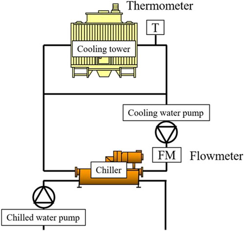
Table 1. Specifications of each unit.

Unit	Rated specifications
Steam absorption chiller	Refrigerating capacity 422 kW (120 USRT)
	Power consumption 2.4 kW
	Steam consumption 432 kg/h
	Cooling water flow rate 2,000 L/min
	Chilled water flow rate 1,008 L/min
Cooling tower	Power consumption 7.5 kW
	Cooling water flow rate 3,000 L/min
Cooling water pump	Cooling water flow rate 1,900 L/min
	Head 18.0 m
	Power consumption 11.0 kW
Chilled water pump	Chilled water flow rate 1008 L/min
	Head 18.0 m
	Power consumption 5.5 kW

The HVAC system consists of a cooling tower, a chiller, a cooling water pump, and a chilled water pump. Inverters control the fan of the cooling tower and the cooling water pump based on the set values of the outlet temperature of cooling water (cooling tower) and the flow rate of cooling water, respectively.

Obtained data

Table 2 shows the data obtained for the target building.

Table 2. Data used in tests.

Item	Unit	Notes
Cooling water supply temperature	°C
Cooling water flow rate	L/min
Chilled water supply temperature	°C
Chilled water calory	MJ/h	Converted to chiller load factor (chilled water calory/refrigerating capacity (1519.2 MJ))
Ambient wet-bulb temperature	°C
Chiller power consumption	kWh	Converted to primary energy (chiller power consumption × 9.76 MJ/kWh)
Chiller steam consumption	kg/h	Converted to primary energy (chiller steam consumption × 2.675 MJ/kg × 1.36 MJ/MJ)
Cooling tower power consumption	kWh	Converted to primary energy (cooling tower power consumption × 9.76 MJ/kWh)
Cooling water pump power consumption	kWh	Converted to primary energy (cooling water pump power consumption × 9.76 MJ/kWh)
Chilled water pump power consumption	kWh	Converted to primary energy (chilled water pump power consumption × 9.76 MJ/kWh)
Operation conditions of each unit	—

The power and steam primary energy factors are 9.76 MJ/kWh and 1.36 MJ/MJ (MEGJ 1998), respectively. The unit caloric value of steam is 2.675 MJ/kg (MEGJ 1998).

Test conditions for training

Yajima et al. (2017) showed that six variables could express the cooling water system of heat source systems: (1) ambient wet-bulb temperature, (2) chiller load factor, (3) cooling water temperature, (4) cooling water flow rate, (5) chilled water temperature, and (6) chilled water flow rate.

Table 3 shows the conditions of the six variables.

Table 3. Conditions of variables.

Ambient wet-bulb temperature	2–28 °C (increments of 2 °C), 14 patterns
Chiller load factor	10–90% (increments of 10%), 9 patterns
Cooling water temperature	20–30 °C (increments of 1 °C)
Cooling water flow rate	1,000–1,900 L/min (increments of 100 L/min)
Chilled water temperature	7 °C
Chilled water flow rate	1,008 L/min

The load-side set points, that is, the chilled water temperature and chilled water flow rate, were fixed to 7 °C and 1008 L/min (rated value), respectively, because the target was the cooling water system alone. Maintaining the chilled water temperature and flow rate condition ensures the thermal comfort of the room. The ambient and loading conditions (i.e., ambient wet-bulb temperature and the chiller load factor) cannot be adjusted manually. Therefore, we changed the cooling water temperature and flow rate. These variables were set for each combination of the ambient wet-bulb temperature and chiller load factor. The total number of combinations of the two was 126. In this facility, the chillers are not used in winter. However, in some buildings, chillers are required all year round. To accommodate such facilities, we conducted experiments with a broader range.

Constraint conditions of a search range

The heat capacity required for the building may not be satisfied when the setpoints for the cooling water temperature and flow rate are searched. For example, a large difference between the inlet and outlet of the chiller’s cooling water temperature should be ensured when the cooling water flow rate is extremely decreased. However, the temperature difference that can be ensured for the HVAC system is limited by its performance. Table 4 shows the constraint conditions of the search ranges of the cooling water temperature and cooling water flow rate.

Table 4. Constraint conditions of search ranges.

Variable	Constraint conditions
Cooling water temperature	Ambient wet-bulb temperature ＋ 1 °C (lower limit, 20 °C) ≤ T ≤ rated temperature (30 °C)
Cooling water flow rate	Chiller load factor × rated flow rate (1900 L/min) (lower limit, 1000 L/min) ≤ F ≤ rated flow rate(1900 L/min)

Conditions for applying Bayesian optimization

In this section, we show the conditions for using Bayesian optimization. The explanatory variables are ambient wet-bulb temperature, chiller load factor, cooling water temperature, cooling water flow rate, chilled water temperature, and chilled water flow rate. The objective variable is the energy consumption per unit production heat rate (hereafter, energy consumption rate). The inputs to the chilled water temperature and flow rate are constants (initial setting). The ambient wet-bulb temperature and the chiller load factor inputs are values of the sensors when setting the central monitoring system. Then, values of the cooling water temperature and flow rate at which Equation 7 is maximized are calculated.

Training flow

Figure 2 shows the control flow using Bayesian optimization.

Fig. 2. Control flow using Bayesian optimization.

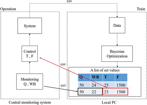
As shown in Figure. 2, the control flow consists of two steps: train and operation. Bayesian optimization obtains the next setpoints for the cooling water temperature and the cooling water flow rate in the training step. Then a list of setpoints of the cooling water temperature and flow rate corresponding to the combination of wet-bulb temperature and load factor is created. The operational data to be obtained include ambient wet-bulb temperature, chiller load factor, cooling water temperature, cooling water flow rate, chilled water temperature, chilled water flow rate, and energy consumption rate. In the operation step, the set values of the cooling water temperature and flow rate corresponding to the wet-bulb temperature and chilled load factor at the setting change are retrieved from the list of set values. Next, the central monitoring system retrieves the set values and the operation is performed. The time interval for changing the operation data and setting values is 1 h. Iterating the two steps enables efficient determination of the optimal set values. The central monitoring system controls the operation by activating and deactivating equipment, and changes setpoints. The learning of this method is calculated on a local PC independent of the central monitoring system. Information on operation data and setpoints is saved in csv format.

Test conditions during demonstration

We compared three control methods in a demonstrative test: our proposed method, model-based control, and control with rated specifications (rated specification control). Life-cycle energy management (LCEM), an energy simulation tool widely used in Japan, has been utilized as a model-based control (Ito et al. 2008). Yajima et al. (2017) created a simulation model (LCEM) using data from the same facility. The optimal control is determined by changing the set values of the cooling water temperature and flow rate in LCEM under various conditions without using the actual facility. The accuracy and energy-saving performance of LCEM in the target facility have already been demonstrated by Yajima et al. The cooling water temperature and flow rate for the rated specification control were 30 °C and 1900 L/min, respectively. The rated specification control is the set value based on the design conditions when the building is constructed. The set value of the rated specification control is designed to respond to high heat loads. Facilities that have not introduced energy-saving technologies to change the set value are operated with the rated specification control. The set values for each control were altered within the intervals shown in Table 5.

Table 5. Intervals of changing set values for different control methods.

	Time
Proposed method	1 h
Model-based control	1 min
Rated specification control	—

The proposed method has a 1-h interval for setting and data collection to accommodate the existing watt-hour meters. Therefore, the setting and data collection interval of the model-based control is 1 min, and this is an optimal control system that has already been put to practical use.

Test process

We carried out training and demonstrative tests. Table 6 shows the training process.

Table 6. Process of training.

	Conditions
Period	June 6, 2019–July 17, 2019
Operation hours	8:00–16:00

In the tests, the HVAC system was operated by rated specification control under the initial conditions of 30 °C and 1900 L/min cooling water on June 6 and 7, 2019. Afterward, operation conditions with less energy consumption were searched by changing the determined set values using Bayesian optimization. The total training period was 20 days (5 days per week). Two hours of startup and shutdown were not used as training data.

Next, the demonstrative test process is shown in Figure 3.

Fig. 3. Demonstrative test process.

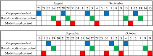
We compared our proposed method, model-based control, and rated specification control in the demonstrative test. The total period of the demonstrative test was 27 days. The control method was switched each day.

Results and discussion

Results of training

Figure 4 shows the distributions of the chiller load factor and the ambient wet-bulb temperature during the training.

Fig. 4. Distributions of chiller load factor and ambient wet-bulb temperature during training.

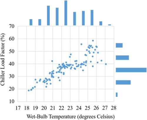
There is no large bias in the distributions, and there is a correlation between the chiller load factor and the ambient wet-bulb temperature. Thus, the results indicate that the outside environment greatly affected the HVAC system rather than the building’s inside atmosphere.

Figure 5 shows the chilled water temperature during the training period.

Fig. 5. Chilled water temperature during training.

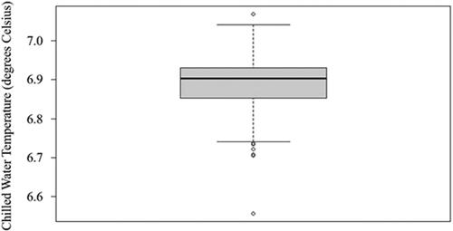
The chilled water temperature is controlled at 7 °C. Since the chilled water temperature can be held at 7 °C, the thermal environment in the room can be considered as maintained.

Figures 6 and 7, respectively, show the mean and variance of the posterior distributions of energy consumption per unit production heat rate (hereafter, energy consumption rate) during training.

Fig. 6. Mean of the posterior distribution of energy consumption rate through training.

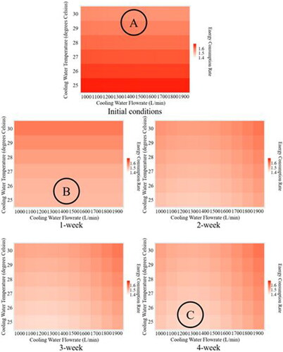
Fig. 7. Variance of the posterior distribution of energy consumption rate through training.

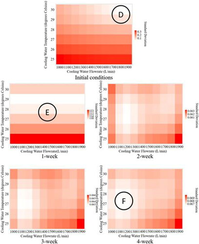
The energy consumption rate is an evaluation index obtained by dividing the total energy consumption rate by the chiller load. Note that the range of variance in Figure 7 is different for each figure.

Figures 6 and 7 were obtained at 40% chiller load factor and 24 °C ambient wet-bulb temperature. The dark red area in the graph indicates a high energy consumption rate, whereas the light red area indicates a low energy consumption rate.

As shown in Figure 6, higher cooling water temperatures (A: light color in the upper area) were considered settings for operation with less energy consumption rate under the initial conditions. Afterward, lower cooling water temperatures were considered a more suitable setting for energy-saving through training (B: the light area moved from the upper part to the lower part). Finally, the optimal conditions were found to be 25 °C cooling water temperature and 1200 L/min cooling water flow rate (C: lower left of the figure); thus, the optimal cooling water flow rate was above its lower limit. As shown in Figure 7, the variance was small only at ∼30 °C cooling water temperature and ∼1900 L/min cooling water flow rate (D: light color in the upper right area) under the initial conditions. The variance of the entire area decreased (E: the color of the entire area became light) as the search proceeded. Finally, the area with a lower energy consumption rate (F: lower left of the figure) was intensively searched. Thus, unknown points that had not been observed were first searched to understand the overall situation; then the areas with lower energy consumption rates were extensively searched.

From these results, we found that the suitable set values for energy saving can be automatically searched through rated specification control using Bayesian optimization.

Results of the demonstrative test

We compared our proposed method, model-based control, and rated specification control. Figure 8 shows the distributions of the chiller load factor and the ambient wet-bulb temperature obtained in the demonstrative test.

Fig. 8. Distributions of chiller load factor and ambient wet-bulb temperature obtained in the demonstrative test.

The means and standard deviations of ambient wet-bulb temperature and chiller load factor in the demonstration experiment are shown in Table 7.

Table 7. The means and standard deviations of ambient wet-bulb temperature and chiller load factor during the demonstrative test.

	Our proposed method	Rated specification control	Model-based control
Chiller load factor [%]	41.4 ± 8.05	39.1 ± 10.58	41.1 ± 13.41
Ambient wet-bulb temperature [°C]	24.4 ± 2.49	24.0 ± 3.43	23.6 ± 3.19

As shown in Figure 8, the ambient wet-bulb temperature and the chiller load factor conditions of the proposed method are slightly biased toward the center compared to the other methods. However, in Table 7, the means of the ambient wet-bulb temperature and chiller load factor are almost the same when the standard deviation is taken into account. These results show that the external factors for the ambient wet-bulb temperature and chiller load factor do not differ among the three methods.

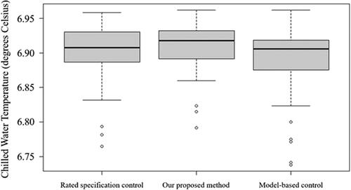
Figure 9 shows the comparison of the chilled water temperature in the demonstrative test. Again, there is almost no difference in the chilled water temperature among the three methods, indicating that the thermal environment in the room can be maintained.

Fig. 9. Chilled water temperature for different control.

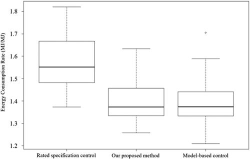
Figure 10 shows the distributions of the energy consumption rate among the three methods. The distributions of energy consumption rate for the rated specification control, our proposed method, and model-based control are shown from left to right. As shown in Figure 10, the median energy consumptions of the proposed method and model-based control are equivalent. However, the lower energy consumption limit in the model-based control is quite low, and there are outliers. This can be attributed to external factors since the model-based control in Figure 8 has a slightly wider distribution of wet-bulb temperature than the proposed method has.

Fig. 10. Distributions of energy consumption rate for different control.

Figure 11 shows the energy consumption rate comparison of the three methods. The energy consumption rates for the rated specification control, our proposed method, and model-based control are shown in Figure 11. The blue, orange, gray, and yellow colors indicate the energy consumption rate of the chiller, cooling tower, cooling water pump, and chilled water pump, respectively. The energy use was reduced by 10.38% for our proposed method and by 11.34% for the model-based control. We carried out a t-test to examine the mean energy consumption rate difference between our proposed method and the model-based control. The obtained values t = 0.10391, df = 106, and p (= 0.9174) > 0.05 show no significant difference. Therefore, our proposed method and model-based control have no major difference in performance. However, in our proposed method, the control settings were changed every 1 h, and the existing sensors can be used, enabling us to widely apply the method to HVAC systems and reduce the cost of its introduction.

Fig. 11. Energy consumption rate for different control.

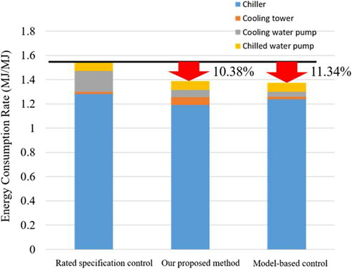
As shown in Figure 11, the proportions of the energy consumption rate for the chiller, cooling tower, and cooling water pump are different between our proposed method and model-based control. This is due to the difference in the optimal set values. In our proposed method, the chiller’s efficiency is increased by decreasing the cooling water temperature to the lower limit, thereby decreasing the proportion of the chiller’s energy consumption rate. On the other hand, the load of the cooling tower fan increases, resulting in the increased energy consumption rate of the cooling tower. Likewise, the energy consumption rate of the cooling water pump increases because the cooling water flow rate is not reduced to the lower limit. In the model-based control, however, the cooling water temperature is not decreased to the lower limit, resulting in the chiller’s reduced efficiency and increased energy consumption rate. In contrast, the load of the fan of the cooling tower decreases and its energy consumption rate decreases. As a result, the energy consumption rate of the cooling water pump decreases because the cooling water flow rate is reduced to the lower limit.

Comparison of energy consumption rate between training and demonstration

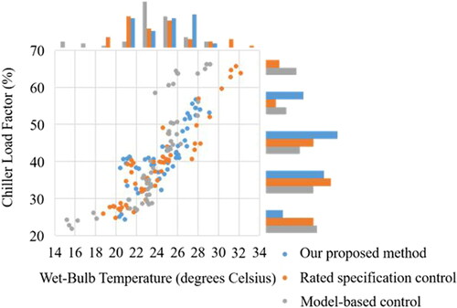
In training, the conditions for energy saving are searched by changing the set values for the cooling water temperature and flow rate. However, this means that the HVAC system is not always operated under energy-saving conditions. Therefore, we compared the energy consumption rate in the training and demonstrative test to verify the energy-saving performance of our proposed method during training. Figure 12 shows the distributions of the chiller load factor and the ambient wet-bulb temperature in the training and demonstrative test.

Fig. 12. Distributions of chiller load factor and ambient wet-bulb temperature.

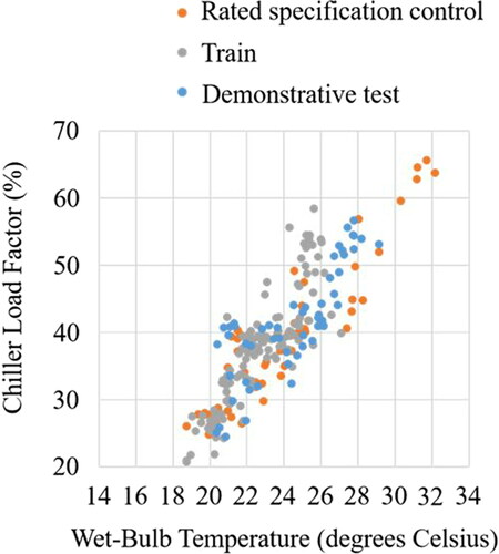
The gray dots are the distribution in training, whereas orange and blue dots indicate the demonstrative test distributions under the rated specification control and using our proposed method, respectively. Thus, there is no bias in the distributions in the training and demonstrative test, although their seasons are different, which shows that the HVAC system is operated at an equivalent ambient wet-bulb temperature and chiller load factor.

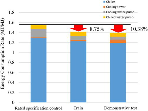
Figure 13 shows a comparison of the energy consumption rate between the training and demonstrative test. It shows the energy consumption rate for the rated specification control, the training, and the demonstrative test. The blue, orange, gray, and yellow colors indicate the energy consumption rate of the chiller, cooling tower, cooling water pump, and chilled water pump, respectively. The energy use was reduced by 8.75% during the training and by 10.37% in the demonstrative test. Thus, a favorable energy-saving rate is achieved in training, although the set values for energy saving are searched by changing them. As shown in Figure 12, the wet-bulb temperature and the load factor of the training process vary from 18 °C to 26 °C and from 20% to 60%, respectively. The total number of conditions that can be set in the training process is 436. We found the equivalent distribution of energy consumption in 2 weeks as in 4 weeks, as shown in Figure 5. The number of times set in 2 weeks is 70 times (2 weeks × 5 days × 7 h). Assuming that we searched 70 out of 436 setting conditions, we could find setting conditions that save energy in 16% of the searches.

Fig. 13. Energy consumption rate in training and demonstrative test.

Conclusion and future work

Conclusion

The training results indicate that the optimal set values can be automatically determined in 4 weeks as the training proceeds under rated specification control with Bayesian optimization. In the training process, unknown points that have not been observed are searched to clarify the overall situation; then the areas with a lower energy consumption rate are intensively searched, enabling an efficient search.

We carried out a demonstrative test to verify the performances of our proposed method, model-based control, and rated specification control. We found that energy use under the rated specification control was reduced by 10.38% for our proposed method and by 11.34% for model-based control. A t-test for our proposed method and model-based control gave values of t = 0.10391, df = 106, and p (= 0.9174) > 0.05, showing equivalent performance between them. The cost of introducing the proposed method can be reduced because the control settings are changed every 1 h, and the existing sensors can be used.

During the training, the energy use was reduced by 8.75% for our proposed method. Thus, a favorable energy-saving rate is achieved, although the set values for energy saving are searched by changing them. This may be because the setting conditions for saving energy are found with fewer search iterations using Bayesian optimization. Thus, we demonstrated that Bayesian optimization is effective for HVAC systems.

Future work

We verified the effectiveness of Bayesian optimization for one-on-one (one cooling tower and one chiller) HVAC systems in this study. In the future, we will carry out demonstrative tests for various buildings by applying our method to the HVAC’s automation system, toward its practical application. Although we fixed the cooling water temperature and flow rate on the load side, these indices should be added to the variables to increase the energy-saving rate further. To this end, the units’ energy consumption, including those on the load side (secondary pumps and air handling unit), should also be optimized. We need to consider the entire building in addition to HVAC systems in our future work.

Disclosure statement

The authors have no conflicts of interest directly relevant to the content of this article.

Additional information

Funding

This work is partly supported by JST CREST Grant Number JPMJCR1761.

References

- Auer, P. 2002. Using confidence bounds for exploitation-exploration trade-offs. Journal of Machine Learning Research 3:397–422. doi:https://doi.org/10.1162/153244303321897663
- Braun, J., and G. Diderrich. 1990. Near-optimal control of cooling towers for chilled-water systems. ASHRAE Transactions 96 (2):806–13.
- Chow, T. T., G. Q. Zhang, Z. Lin, and C. L. Song. 2002. Global optimization of absorption chiller system by genetic algorithm and neural network. Energy and Buildings 34 (1):103–9. doi:https://doi.org/10.1016/S0378-7788(01)00085-8
- Cui, C., X. Zhang, W. Cai, and F. Cheng. 2021. A novel air balancing method for HVAC systems by a full data-driven duct system model. IEEE Transactions on Industrial Electronics 68 (12):12595–606. doi:https://doi.org/10.1109/TIE.2020.3040685
- Deng, J., and H. Wang. 2018. Modeling and optimizing building HVAC energy systems using deep neural networks. 2018 International Conference on Smart Grid and Clean Energy Technology, Kajang, Malaysia, 181–5. doi:https://doi.org/10.1109/ICSGCE.2018.8556684
- Frazier, P., W. Powell, and S. Dayanik. 2009. The knowledge-gradient policy for correlated normal beliefs. INFORMS Journal on Computing 21 (4):599–656. doi:https://doi.org/10.1287/ijoc.1080.0314
- Goodfellow, I., Y. Bengio, and A. Courville. 2016. Deep learning. Cambridge, Massachusetts: MIT Press.
- Hennig, P., and C. J. Schuler. 2021. Entropy search for information-efficient global optimization. Journal of Machine Learning Research 13:1809–37.
- Hino, H. 2021. Active learning: Problem settings and recent developments. ArXiv:2012.04225.
- Ignjatovic, M. G., B. D. Blagojevic, M. M. Stojiljkovic, D. M. Mitrovic, and A. S. Andelkovic. 2016. Optimization of HVAC system operation based on a dynamic simulation tool. REHVA Journal 53 (6):56–62.
- Ito, M., S. Murakami, M. Okumiya, S. Tokita, H. Niwa, Y. Suigihara, H. Tanaka, T. Watanabe, M. Yoshinaga, K. Miura, et al. 2008. Development of HVAC system simulation tool for life cycle energy management Part 1: Concept of life cycle energy management and outline of the developed simulation tool. Building Simulation 1 (2):178–91. doi:https://doi.org/10.1007/s12273-008-8209-6
- Japanese Government. 2021. Expert panel on climate change. Accessed June 3, 2021. https://japan.kantei.go.jp/99_suga/actions/202105/_00017.html.
- Jones, D. R., M. Schonlau, and W. J. Welch. 1998. Efficient global optimization of expensive black-box functions. Journal of Global Optimization 13 (4):455–92. doi:https://doi.org/10.1023/A:1008306431147
- Konzen, E., Y. Cheng, and J. Q. Shi. 2021. Gaussian process for functional data analysis: The GPFDA package for R. ArXiv: 2102.00249.
- Kuroha, R., Y. Fujimoto, W. Hirohashi, Y. Amano, S. Tanabe, and Y. Hayashi. 2018. Operation planning method for home air-conditioners considering characteristics of installation environment. Energy and Buildings 177:351–62. doi:https://doi.org/10.1016/j.enbuild.2018.08.015
- Kushner, H. J. 1964. A new method of locating the maximum point of an arbitrary multipeak curve in the presence of noise. Journal of Basic Engineering 86 (1):97–106. doi:https://doi.org/10.1115/1.3653121
- Ministry of the Environment Government of Japan. 1998. Law concerning the promotion of the measures to cope with global warming. Accessed June 3, 2021. https://www.env.go.jp/en/laws/global/warming.html#:∼:text=%22Measures%20to%20cope%20with%20global,greenhouse%20gas%20emissions%20and%20to.
- Ministry of the Environment Government of Japan. 2020. Submission of Japan's Intended Nationally Determined Contribution (INDC). Accessed June 3, 2021. https://www.env.go.jp/en/earth/cc/2030indc.html.
- Mockus, J. 1974. On Bayesian methods for seeking the extremum. Proceedings of the IFIP Technical Conference, Novosibirsk, Russian, 400–4.
- Qiu, S., Z. Li, Z. Li, J. Li, S. Long, and X. Li. 2020. Model-free control method based on reinforcement learning for building cooling water systems Validation by measured data-based simulation. Energy and Buildings 218:110055. doi:https://doi.org/10.1016/j.enbuild.2020.110055
- Rasmussen, C. E., and C. K. I. Williams. 2005. Gaussian processes for machine learning. Tokyo, Japan: The MIT Press.
- Schölkopf, B., and A. J. Smola. 2001. Learning with kernels. Bonn, Germany: MIT Press.
- Shahriari, B., K. Swersky, Z. Wang, R. P. Adams, and N. D. Freitas. 2016. Taking the human out of the loop: A review of Bayesian optimization. Proceedings of the IEEE 104 (1):148–75. doi:https://doi.org/10.1109/JPROC.2015.2494218
- Sutton, R., and A. Barto. 1998. Reinforcement learning: An introduction. Georgia, United States: MIT Press.
- Suzuki, S., S. Takeno, T. Tamura, K. Shitara, and M. Karasuyama. 2020. Multi-objective Bayesian optimization using Pareto-frontier entropy. Proceedings of the 37th International Conference on Machine Learning, Vienna, Austria, Vol. 119, 9279–88. arXiv:1906.00127
- Telsang, B., M. Olama, S. Djouadi, J. Dong, and T. Kuruganti. 2019. Stability analysis of model-free control under constrained inputs for control of building HVAC systems. 2019 American Control Conference, United States, 5879–5883. doi:https://doi.org/10.23919/ACC.2019.8815381
- The Energy Conservation Center in Japan. 2018. Energy conservation for office buildings. Accessed June 3, 2021. https://www.asiaeec-col.eccj.or.jp/wpdata/wp-content/uploads/2018/03/office_building.pdf.
- United Nations. 2015. Paris agreement. Le Bourget, France: United Nations.
- Wada, T., and H. Hino. 2019. Bayesian optimization for multi-objective optimization and multi-point search. arXiv:1905.02370.
- Wang, S., and Z. Ma. 2008. Supervisory and optimal control of building HVAC systems: A review. HVAC&R Research 14 (1):3–32. doi:https://doi.org/10.1080/10789669.2008.10390991
- Yajima, K., Y. Akashi, Y. Kuwahara, and M. Fukui. 2017. Study of optimal operation for an HVAC system part 1 Optimization of cooling water temperature set point and verification of energy saving effects by actual measurement. Transactions of the Society of Heating, Air-Conditioning and Sanitary Engineers of Japan 248:11–9. doi:https://doi.org/10.18948/shase.42.248_11
- Zhang, X., M. Pipattanasomporn, T. Chen, and S. Rahman. 2020. An IoT-based thermal model learning framework for smart buildings. IEEE Internet of Things Journal 7 (1):518–27. doi:https://doi.org/10.1109/JIOT.2019.2951106