Experimental validation of the dynamic thermal network approach in modeling buried pipes

Abstract

The transient behavior of buried pipe systems plays a significant role in many heating and cooling systems, particularly in thermal energy networks and ground heat exchangers. In this study, the dynamic thermal network (DTN) approach’s validity as a response factor method in modeling dynamic conduction heat transfer in a buried pipe system is experimentally validated. A lab-scale representation of a buried pipe system has been excited by step changes in boundary temperatures and heat fluxes measured up to times approaching steady-state conditions. This data is used to derive weighting factors and also evaluate the validity of numerical representations of the buried pipe and to verify that the DTN method can reproduce the heat flux responses. It is demonstrated that the weighting factors required in this method can be derived from both numerical and experimental step-response time series data. The DTN method is found to be both accurate in reproducing the heat fluxes in the validation experiments but also significantly more computationally efficient than a conventional numerical model when simulating long timescale responses in buried pipe systems.

Introduction

There are many thermal engineering applications where the evaluation of the dynamic heat exchange between the buried pipes and the ground is essential. In district heating and cooling (DHC) systems, the assessment of dynamic heat losses in buried pipe distribution networks is one of the significant factors in the simulation and optimization of such systems and subsequent economic evaluation (Danielewicz et al. 2016; Guelpa 2020). The dynamic behavior of the buried pipe network furthermore affects the control and management of operational DHC systems (Dénarié, Aprile, and Motta 2019). Recently, a number of new DHC system concepts have been proposed in which the role of the transient heat behavior of pipe systems is even more important (Meibodi and Loveridge 2022). The main common characteristic of these proposed concepts is reductions of the distribution temperatures in order to enable the DHC system to be integrated with a higher share of low-temperature heat sources, and decrease the overall heat losses of the systems (Lund et al. 2018). Using relatively low temperatures in the pipe systems, along with the use of fluctuating low-temperature heat sources makes it essential to use a suitable dynamic model to design the system and evaluate whether heat delivery meets the requirements of end-users to provide comfort in buildings at all times.

Various types of ground heat exchangers–-typically implemented as a part of ground source heat pump (GSHP) or borehole thermal energy storage systems–-are also applications in which the dynamic thermal behavior of buried pipe systems is significant (Naicker and Rees 2018; Zhang, Gong, and Zeng 2021). Ground heat exchangers (GHE) consist of heat exchanger pipes that extract/reject heat from/to circulating fluid to/from the grout and surrounding ground via transient conduction process (Rees 2016). They can be implemented either vertically in borehole heat exchangers (BHE) or horizontally in shallow horizontal heat exchangers. The physical processes in horizontal ground heat exchange systems are similar to that in DHC systems – the main difference being the use of pipe insulation in the latter. Consequently, the modeling method and experimental validation are also applicable to modeling such horizontal systems and horizontal pipes in larger BHE arrays.

In addition to district heating and cooling systems and ground heat exchangers, the dynamic heat exchange between the buried pipes and the ground is of interest in many other engineering applications, such as the evaluation of the heat losses from arrays of the buried electric cables (Ocłoń et al. 2018), underground thermal energy storage (UTES) (Dahash et al. 2020), subway tunnels (Vasilyev, Peskov, and Lysak 2022)}, and oil pipeline (Chen et al. 2021). In the following, an overview of previous literature on the topic of modeling the dynamic thermal behavior of buried pipe systems is provided.

In the early studies on the modeling heat losses of buried pipes using analytical approaches in steady-state conditions, a number of simplifications and assumptions have been made (Bennet, Johan, and Hellström 1987). In these studies, the ground is generally conceived as a semi-infinite solid in which the pipes are buried with isothermal or uniform heat flux boundary conditions (Thiyagarajan and Yovanovich 1974). Bau and Sadhai (1982) presented an analytical solution for calculating heat losses from a buried pipe in the ground that used a mixed convective boundary condition with a uniform heat transfer coefficient. Bøhm (2000) developed an approach where the transient heat loss is determined using the steady-state heat loss equations and the undisturbed ground temperature. An experiment consisting of insulated and uninsulated pipe buried in the ground was used to validate the method against the measured ground temperatures at different locations. Recently, van der Heijde, Aertgeerts, and Helsen (2017) presented an analytical model for a fast simulation of steady-state heat losses in double pipes in DHC systems. However, the model cannot deal with the dynamic behavior of the buried pipes.

The development of fast and affordable computers has led to the introduction of numerous numerical approaches to modeling the dynamic heat losses of buried pipe systems. The approaches widely applied to calculate transient ground conduction have been the Finite Element Method (FEM) (Gabrielaitiene, Bøhm, and Sunden 2008; Dalla Rosa, Li, and Svendsen 2011; Dalla Rosa, Li, and Svendsen 2013) or the Finite Volume Method (FVM) (Rees 2015; Arabkoohsar, Khosravi, and Alsagri 2019; Guelpa and Verda 2019). Gabrielaitiene, Bøhm, and Sunden (2008) investigated the implementation of the FEM in modeling the heat propagation in the buried pipes of DHC systems. They demonstrated that the models fail to sufficiently stimulate the peak values and temperature response time due to the pipe inlet condition changes. In another study, Khosravi and Arabkoohsar (2019) presented a thermal-hydraulic model using the FVM to investigate the potential of buried twin-pipes configurations in the implementation of the various proposed district heating systems. They showed the thermal inertia of the buried pipe and surrounding soil plays an important role in the dynamic modeling of such systems and needs to be taken into account in the design of future DHC systems.

In both numerical modeling approaches, due to the high computational efforts required, either some simplifications are made such as reducing the order of the thermal problem, which adversely affects the accuracy, or the implementations are limited to less practical cases. Often computational costs mean FVM or FEM approaches are not practical for routine dynamic heat loss analysis of the buried pipes with the long series of data involved in the seasonal analysis.

The approach implemented in this research to modeling the dynamic heat transfer of the buried pipes is the Dynamic Thermal Network (DTN) method. This approach is classified as a response factor method that represents the transient conduction processes as a network (in the sense of nodes connected by resistances) in which boundary heat fluxes and temperatures can be calculated between multiple surfaces of a conducting body. This approach has been first developed by Claesson (2002) for the simulation of heat transfer in building fabric components and was originally extended from the network representation of the steady-state conduction process (Claesson 2003). This approach has been successfully implemented in modeling a number of thermal engineering applications (Wentzel 2005). Significant advantages are that the geometry can be complex and heterogeneous – situations that are difficult to deal with in analytical models – yet is mathematically exact.

Fan, Rees, and Spitler (2013) applied the dynamic thermal network method for modeling foundation heat exchangers (FHE) and showed how more complex boundary conditions related to the pipes and ground surface could be implemented. The model implemented as a compact horizontal ground heat exchanger was validated with experimental data from an installation at an experimental house. Shafagh et al. (Shafagh and Rees 2018; Shafagh et al. 2020) implemented the DTN approach in modeling a diaphragm wall ground heat exchanger and validated the model using full-scale in-situ measurements of overall heat transfer. The levels of agreement in the predicted dynamic behavior of the system using the model and measurement data are concluded to be more than satisfactory for design and thermal analysis purposes of diaphragm wall heat exchangers. In another study, Rees and Van Lysebetten (2020) developed a model using the DTN approach to model the long-term thermal performance of the energy piles. The model was validated with the measured data collected over several months from a test pile installation and shown to be able to represent conditions effectively in a computationally efficient manner suitable for the design and simulation of such systems.

One of the main features of the DTN approach in its discretized form, is that the current state of the thermal system is entirely expressed in terms of current and past temperatures modified by corresponding weighting factors. Hence, it is necessary to calculate the weighting factor series for each geometry and set of thermal properties a priori. This is done by analysis of the heat fluxes in response to a step change in boundary temperatures. The method itself is not dependent on any particular model or set of measurements to calculate these heat fluxes. Derivation of the weighting factors in all previous studies was carried out either using analytical or numerical models to calculate the step response heat fluxes. Numerical approaches are more able to deal with complex geometries but can require significant computational effort although the weighting factors only have to be calculated once for each problem. Although it has not been attempted before, it is possible to derive the weighting factors from experimentally derived heat flux time series data. The challenge is chiefly to be able to apply step changes at the boundaries of the experiment. We have attempted to do this for a buried pipe case and report on it below.

Considering the flexibility and efficiency of the DTN approach in representing the time-varying boundary conditions of any arbitrary three-dimensional geometry have motivated us to experimentally verify the approach with a focus on a buried pipe system. Overall suitability of the approach to model such applications also depend on whether a pure conduction model of heat transfer is adequate for granular materials and whether assuming the response can be modeled with a 2D numerical representation of a cross-section is appropriate. We address these questions by comparing corresponding experimental and both 2D and 3D numerical results.

Previous work on the development of a model of buried pipe systems had focused on short time-scale response associated with the fluid behavior in pipes with and without insulation (Meibodi and Rees 2020). The aim is to combine the model of short time-scale response with that of the DTN model to deal with the long timescale response associated with conduction through the ground (Meibodi 2020). In this paper we focus on the latter.

Model development

In this research, two modeling approaches have been implemented: finite volume models (FVM) and a dynamic thermal network (DTN) model. The Dynamic Thermal Network (DTN) model has been developed to represent the dynamic heat transfer in the buried pipeline system and has been tested considering both experimentally and numerically derived weighting factor series. The model is then validated against the experimental data. An overview of the DTN approach and the theoretical basis of the weighting function derivation are described in Section 2.1.

The FVM approach has been applied firstly in the form of a three-dimensional buried pipeline and pipe fluid model using a conjugate heat transfer solver that is used to solve both fluid flow and conduction heat transfer conditions. This model is presented in Section 3.2. This model (three-dimensional FVM) is used to represent the buried pipe system with the least possible assumptions with the ability to simulate any three-dimensional effects and fluid conditions explicitly.

A two-dimensional form of FVM has also been implemented that solves the transient conduction equation in the solid domain and uses convective boundary conditions. This is the form of the model intended to be used in practice to derive the weighting function series required in the DTN model. Comparing the results of both numerical models with the experiments allows the significance of any 3D effects and the adequacy of a 2D representation to be evaluated.

Dynamic thermal network representation

There are a number of potential advantages of the DTN approach in dealing with problems of transient conduction with embedded pipes. The particular advantages can be summarized as: (i) representation of arbitrary three-dimensional geometries with heterogeneous thermal properties; (ii) computational efficiency in problems with long time constants such as ground-coupled problems, and; (iii) allowing multiple boundary conditions on complex surfaces to be included. The theoretical basis of the approach is described in some detail elsewhere (Claesson 2002; Fan, Rees, and Spitler 2013). Here, we give an overview of the method and explanations of the role of the weighting factor data.

It should be noted that the DTN method is, in principle, able to deal with boundary conditions applied at any number of surfaces. Practical engineering problems can be usually dealt with by implementing the method with either two or three surfaces. A DTN model of district heating pipes is achievable with a three-surface formulation if both flow and return pipes are included along with the ground surface. For the sake of the validation in this study, we have limited the problem to a single buried pipe and so two-surface formulation as set out below. The method is readily extensible and so implementing a second adjacent pipe is straightforward (Rees and Van Lysebetten 2020; Shafagh et al. 2020).

In a two-surface implementation of the DTN approach for a buried pipe, the surfaces at which convective (mixed) boundary conditions are defined are illustrated in Figure 1. The first is that of the pipe with time-dependent boundary temperature (T₁) and the second is the ground with boundary temperature (T₂). The heat flows from/to the pipes to/from the ground are denoted by Q₁(t), Q₂(t) respectively. It should be noted that the temperatures (T_i(t)) and fluxes (Q_i(t)) of the dynamic network are defined at the boundary temperature nodes with convective (mixed) boundary conditions, i.e. temperatures adjacent to the surface rather than at the surfaces themselves. Accordingly, the terms "boundary" and "surface" are distinct in this method.

Fig. 1. Dynamic thermal network representing the buried pipe in the ground.

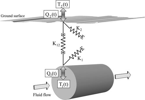
In the DTN approach, each temperature of the boundary is considered as a node that is connected with all other boundary temperature nodes in a network of resistances (The network is trivial in a two-surface problem and a delta form in a three-surface problem). In this case, there are two-surface thermal conductances K₁ and K_2, for the buried pipe, and the ground surface, respectively. The surface thermal conductances can be calculated by multiplying the surface area (A) in the heat transfer coefficient (h), e.g. K₁₌ A_1. h_1. The other thermal conductance in the heat transfer path between the nodes is (K₁₂) which is defined as the inverse of total thermal resistance between the two surfaces in a steady-state condition: K₁₂₌ 1/R₁₂.

In this research, the heat transfer coefficient of the pipeline is determined based on the measured flow rate and Reynolds number of the fluid flow using the well-known Gnielinski’s correlation (Gnielinski 1976). Gnielinski’s correlation has demonstrated its ability to well approximate the experimental data compared with other correlations, particularly for low-Reynolds turbulent fluid flows in a number of studies (Li et al. 2016; Taler and Taler 2017). Accordingly, this correlation has been chosen for the calculation of the heat transfer coefficient of the pipeline. The heat transfer coefficient of the ground surface is obtained experimentally based on the surface heat flux and temperature measurements discussed further in Sections 4 and 5.

The boundary temperatures and fluxes in the DTN approach are calculated based on the weighted average current and previous temperatures at the boundaries. To indicate this, the reversed summation symbols $(\mathrm{\Sigma })$ are used in the network diagrams (Claesson’s notation) adjacent to the conductances, as illustrated in Figure 1.

The main feature of the DTN approach is that the heat fluxes are separated into the admittive (or absorptive) and transmittive components. Admittive fluxes are associated with the temperature changes at that boundary alone. For instance, at an ideally adiabatic surface, the fluxes are totally admittive, and there is no transmittive flux. Transmittive fluxes are associated with heat transfer from one surface to another depending on the temperature differences between them. Generally, in the transient heat transfer process, both components are present at the surfaces, until the steady-state is approached in which the admittive components become zero. For the buried pipe application, the heat flux at each surface consists of one admittive heat flux (Q_1a(t), Q_2a(t)) and one transmittive heat flux (Q₁₂ = Q₂₁), which are expressed as: (1) $$\begin{array}{c}{Q}_1\left(t\right)=\mathrm{ }{Q}_{1a}\left(t\right)+Q_{12}\left(t\right)\\ Q_2\left(t\right)=\mathrm{ }{Q}_{2a}\left(t\right)+Q_{21}\left(t\right)\end{array}$$(1)

The dynamic relationship between boundary temperatures and heat fluxes has a formulation analogous to the steady-state form and can be given in terms of current boundary and averaged temperatures as follows (Claesson 2002): (2) $$\begin{array}{c}{Q}_1\left(t\right)=\mathrm{ }{K}_1\mathrm{ }\left[T_1\left(t\right)-\overline{T_{1a}}\left(t\right)\right]+\mathrm{ }{K}_{12}\mathrm{ }\left[\overline{T_{12}}\left(t\right)-\overline{T_{21}}\left(t\right)\right]\\ Q_2\left(t\right)=\mathrm{ }{K}_2\mathrm{ }\left[T_2\left(t\right)-\overline{T_{2a}}\left(t\right)\right]+\mathrm{ }{K}_{12}\mathrm{ }\left[\overline{T_{21}}\left(t\right)-\overline{T_{12}}\left(t\right)\right]\end{array}$$(2)

While T₁(t), T₂(t) are the current temperatures at the boundaries, $\overline{T_{1a}}\left(t\right), \overline{T_{2a}}\left(t\right)$ are the admittive average temperatures and $\overline{T_{12}}\left(t\right)$ is the transmittive average temperature. The general form of the temperature differences in Equation 2(2) $$\begin{array}{c}{Q}_1\left(t\right)=\mathrm{ }{K}_1\mathrm{ }\left[T_1\left(t\right)-\overline{T_{1a}}\left(t\right)\right]+\mathrm{ }{K}_{12}\mathrm{ }\left[\overline{T_{12}}\left(t\right)-\overline{T_{21}}\left(t\right)\right]\\ Q_2\left(t\right)=\mathrm{ }{K}_2\mathrm{ }\left[T_2\left(t\right)-\overline{T_{2a}}\left(t\right)\right]+\mathrm{ }{K}_{12}\mathrm{ }\left[\overline{T_{21}}\left(t\right)-\overline{T_{12}}\left(t\right)\right]\end{array}$$(2) can be defined in terms of the current temperature and the average temperatures defined by weighted temperature histories for two surfaces as given below: (3) $$\begin{array}{l}\left[\overline{T_{ij}}\left(t\right)-\overline{T_{ji}}\left(t\right)\right]={\int }_0^{\mathrm{\infty }}{\mathrm{\kappa }}_{ij}\left(\mathrm{\tau }\right).\left[T_i\left(t\text{-}\mathrm{\tau }\right)-T_j\left(t\text{-}\mathrm{\tau }\right)\right]d\tau \\ \left[T_i\left(t\right)-\overline{T_{\mathrm{ia}}}\left(t\right)\right]=T_i\left(t\right)-{\int }_0^{\mathrm{\infty }}{\kappa }_{ia}\left(\tau \right).T_i\left(t-\tau \right)d\tau \end{array}$$(3) where ${\mathrm{\kappa }}_{ia}$ and ${\mathrm{\kappa }}_{ij}$ are admittive and transmittive weighting functions. This formulation is mathematically exact for any solid body. For practical applications, we use a discrete form of these equations that is exact for piece-wise linear varying boundary conditions. It is worth noting that the weighting functions are positive (or zero) and the integral of weighting functions is always equal to one: (2) $${\int }_0^{\mathrm{\infty }}{\kappa }_{ia}\left(\tau \right)={\int }_0^{\mathrm{\infty }}{\kappa }_{ij}\left(\tau \right)=1$$(2)

Generally, the admittive weighting functions $\left({\mathrm{\kappa }}_{ia}\left(\mathrm{\tau }\right)\right)$ drops from high values at the beginning to zero at $\mathrm{\tau }=\mathrm{\infty }.$ On the other hand, the transmittive weighting functions $\left({\mathrm{\kappa }}_{ij}\left(\mathrm{\tau }\right)\right)$ firstly increases from zero to a maximum value, then steadily decreases to zero at $\mathrm{\tau }=\mathrm{\infty }.$

Discretization and weighting factor calculation

The convenient approach to deriving the weighting functions is to apply step changes in boundary temperatures and evaluate the heat fluxes from the surfaces due to each step change. For this purpose, at $\mathrm{\tau }=\mathrm{\infty },$ while the temperatures of all surfaces are kept at zero, the boundary temperature of one surface is changed from zero to one. This is repeated for each surface to derive all the sets of weighting factor data.

At the beginning of applying the step change at boundary one, the heat flux from the surface is totally admittive, and its value is equal to K₁. As time proceeds, the admittive flux from the surface decreases, and the transmittive fluxes rise. The admittive flux becomes the difference between the total heat flux from the surface and the transmittive flux between surfaces. As time is approaching the steady-state condition time, the admittive flux approaches zero, and heat flux values between surfaces reach steady-state thermal conductance. Claesson showed that the weighting factors are then related to the gradients of the step response, as given below (Claesson 2003): (5) $$\begin{array}{l}{\kappa }_{ia}\left(\tau \right)=\frac{-1}{K_i}\frac{Q_{\mathrm{i}a}\left(\tau \right)}{\mathrm{d}\tau }\\ {\kappa }_{ij}\left(\tau \right)=\frac{-1}{K_{ij}}\frac{Q_{\mathrm{i}j}\left(\tau \right)}{\mathrm{d}\tau } \end{array}$$(5)

For practical application in simulation calculations, a discrete form of the DTN heat balance and temperature relationships are needed and the weighting factor functions need to be replaced by data series. Claesson showed how this is straightforward. The continuous functions of Equation 3(3) $$\begin{array}{l}\left[\overline{T_{ij}}\left(t\right)-\overline{T_{ji}}\left(t\right)\right]={\int }_0^{\mathrm{\infty }}{\mathrm{\kappa }}_{ij}\left(\mathrm{\tau }\right).\left[T_i\left(t\text{-}\mathrm{\tau }\right)-T_j\left(t\text{-}\mathrm{\tau }\right)\right]d\tau \\ \left[T_i\left(t\right)-\overline{T_{\mathrm{ia}}}\left(t\right)\right]=T_i\left(t\right)-{\int }_0^{\mathrm{\infty }}{\kappa }_{ia}\left(\tau \right).T_i\left(t-\tau \right)d\tau \end{array}$$(3) for the current time step (n) and sequence of previous time steps ($\rho$) as shown in Figure 2, can be expressed in a discrete form as follows (Fan, Rees, and Spitler 2013): (6) $$\begin{array}{l}\left[\overline{T_{ij,n}}\left(t\right)-\overline{T_{ji,n}}\left(t\right)\right]={\sum }_{\rho =0}^{\mathrm{\infty }}{\kappa }_{ij,\rho }.\left[T_{i,n-\rho }-T_{j,n-\rho }\right]\\ \left[T_{i,n}\left(t\right)-\overline{T_{ia,n}}\left(t\right)\right]=T_{i,n}\left(t\right)-{\sum }_{\rho =1}^{\mathrm{\infty }}{\kappa }_{ia,\rho }.T_{i,n-\rho }\end{array}$$(6)

Fig. 2. Character of the admittive fluxes of pipe surface (solid-line) resulting from an unit step change, with the average admittive fluxes (dot-line), and bars representing the average value over each time step.

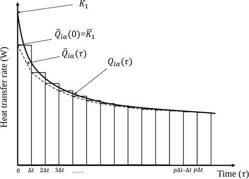
The admittive and transmittive response fluxes resulting from imposing step changes to the boundary conditions can be averaged over each time-step to find the weighting factor series. Considering piecewise linear boundary temperature variations, the weighting factors for the time step $(\mathrm{\Delta }t)$ can be calculated by dividing the average fluxes ($\overline{Q_{ia}},$ $\overline{Q_{ij})}$ over each time step by the modified surface conductances, as given below: (7) $$\begin{array}{c}{\kappa }_{ia,p}=\frac{\overline{Q_{ia}}\left(\rho \mathrm{\Delta }t\text{-}\mathrm{\Delta }t\right)-\overline{Q_{ia}}\left(\rho \mathrm{\Delta }t\right)}{\overline{K_i}}\\ {\kappa }_{i\mathrm{j},p}=\frac{\overline{Q_{\mathrm{ij}}}\left(\rho \mathrm{\Delta }t\text{-}\mathrm{\Delta }t\right)-\overline{Q_{\mathrm{ij}}}\left(\rho \mathrm{\Delta }t\right)}{\overline{K_{i\mathrm{j}}}}\end{array}$$(7)

Here, the surface conductances $\overline{K_{}}$ are modified using the data at the initial step as follows: (8) $$\overline{K_i}=\overline{Q_{ia}}\left(0\right)$$(8)

The admittive step response fluxes ${(Q}_{ia})$ over each time step ($\mathrm{\Delta }t)$ are illustrated for the step applied at a pipe surface in Figure 2.

Note that the origin of the step response heat flux data is not defined in the DTN formulation. Hence, any approaches suitable for step response heat flux series calculation can be used: it can be from an analytical or numerical model. Analytical models are useful for simple geometries (e.g. building walls) and numerical models are more suited to complex geometries. We demonstrate later that experimentally derived heat flux time series can also be used.

Model implementations

DTN model implementation

The DTN method described in this research consists of three main calculation processes: (i) step-response flux calculations, (ii) weighting factors derivation, and (iii) the model simulation process. In a two-surface problem such as this, two step response calculations (sets of data) are needed with different boundary conditions to complete the first stage of this process. In one case the step in boundary temperature is applied at the pipe boundary (fluid temperature) and the ground boundary is held with a constant temperature of zero. In the second case the pipe boundary is fixed at zero and the step, in boundary temperature is at the ground. The transmitted fluxes are the same in each case but the admittive fluxes are different. Consequently, there are three flux time series as a result of two step response calculations (or experiments) and these are used to derive (using Equation 7(7) $$\begin{array}{c}{\kappa }_{ia,p}=\frac{\overline{Q_{ia}}\left(\rho \mathrm{\Delta }t\text{-}\mathrm{\Delta }t\right)-\overline{Q_{ia}}\left(\rho \mathrm{\Delta }t\right)}{\overline{K_i}}\\ {\kappa }_{i\mathrm{j},p}=\frac{\overline{Q_{\mathrm{ij}}}\left(\rho \mathrm{\Delta }t\text{-}\mathrm{\Delta }t\right)-\overline{Q_{\mathrm{ij}}}\left(\rho \mathrm{\Delta }t\right)}{\overline{K_{i\mathrm{j}}}}\end{array}$$(7) ) the weighting factor series ${\kappa }_{1a,p},$ ${\kappa }_{2a,p}, {\kappa }_{12,p}.$ This data is stored for use in any further simulation calculations.

The heat balance equation used to find the time-varying heat fluxes from the boundary temperatures in a simulation is simply found from the application of Equation 2(2) $$\begin{array}{c}{Q}_1\left(t\right)=\mathrm{ }{K}_1\mathrm{ }\left[T_1\left(t\right)-\overline{T_{1a}}\left(t\right)\right]+\mathrm{ }{K}_{12}\mathrm{ }\left[\overline{T_{12}}\left(t\right)-\overline{T_{21}}\left(t\right)\right]\\ Q_2\left(t\right)=\mathrm{ }{K}_2\mathrm{ }\left[T_2\left(t\right)-\overline{T_{2a}}\left(t\right)\right]+\mathrm{ }{K}_{12}\mathrm{ }\left[\overline{T_{21}}\left(t\right)-\overline{T_{12}}\left(t\right)\right]\end{array}$$(2) . At each step in a simulation the average temperatures are updated by applying the weighting factors to the temperatures at previous steps. This makes the simulation of long time series (e.g. seasonal analysis of a DHC network) very computationally efficient. In the work reported here, it has only been necessary to work with boundary conditions using constant heat transfer coefficients. More complex, time-varying, and nonlinear boundary conditions can be dealt with in DTN models and are explained elsewhere (Fan, Rees, and Spitler 2013; Rees and Fan 2013).

Finite volume model implementation

In this research, the finite volume models (FVM) have been developed using the OpenFOAM library (Weller et al. 1998) based on the geometry, boundary and initial conditions of the buried pipeline system in the experimental studies presented in Section 4. The aim has been to develop two FVM models: one to represent the dynamic thermal behavior of the complete three-dimensional buried pipe system including the fluid; a two-dimensional model to derive the weighting function series.

Three-dimensional numerical model

A three-dimensional model of conjugate heat transfer representing the experimental geometry and properties has been developed. In this model, the outer limits of the computational domain are considered the lines of insulation and exposed surfaces. If the model is used to model real design conditions, the boundary would need to be much bigger, i.e. include more ground below and to the side. However, according to the thermal properties of the materials in the experimental apparatus as well as the relatively low temperatures of the step changes, these boundary conditions can be suitably used. More details on the geometry of the experimental apparatus and their materials are presented in Section 4.

In the three-dimensional conjugate heat transfer model, the flow is assumed incompressible, Newtonian, three-dimensional and (low-Reynolds) turbulent. To solve the governing Navier-Stokes and energy equations in this model, a first-order scheme is exploited to discretize the temporal term, and a second-order scheme is employed to discretize the convection and diffusion terms of the governing equations. To model the turbulent flow in the pipe, the well-known $k\text{-}\mathrm{\omega }$ Shear Stress Transport ($k\text{-}\mathrm{\omega }-\mathit{SST}$) model is applied in this work. The energy equation is solved simultaneously in both solid and fluid domains to examine the combination of convection and conduction effects.

In the three-dimensional pipe system numerical mesh, the fluid flow domain is represented by a cylindrical block with a dense mesh near the pipe wall. The pipe wall is represented by a thin cylindrical block with several layers close to the fluid and ground blocks. The ground is represented by a rectangular block with a long length representing the soil surrounding the long-buried pipe. The top of the ground block is exposed to the ambient environment with heat transfer defined by a fixed heat transfer coefficient. The representation of the buried pipe system is displayed in Figure 3.

Fig. 3. A multi-block structured mesh representing a buried pipe system.

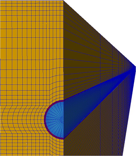
The mesh of the pipe region in the three-dimensional model of conjugate heat transfer used in this research (Figure 3), was refined and validated using published turbulent flow velocity profile experimental data (Eggels et al. 1994; Peng et al. 2018) and comparing numerical convection coefficients with empirical correlation values. Further details are available in the related thesis (Meibodi 2020).

Two-dimensional numerical model

In the two-dimensional FVM model, the transient conduction heat transfer in the buried pipe system is modeled without explicitly modeling the fluid flow. In this model, a fixed heat transfer coefficient is applied to the inside pipe in a mixed boundary condition to take into account the pipe wall heat interaction with the fluid flow. This model uses a similar mesh to that in Figure 3 but in a 2D form and without the fluid flow region). The simulation results from both finite volume models and the DTN model in which the weighting factors are obtained numerically and experimentally are presented and discussed in Section 5.

Experimental design

In this research, an experimental facility was designed and constructed for two main purposes: (i) to validate the DTN model and detailed 3D model with the reliable experimental data (ii) to determine the step response heat flux series for the buried pipe and ground surface in order to derive the weighting factor values. Derivation of the weighting factor values is carried out by measuring the heat flux at the pipe and ground surfaces resulting from imposing the step boundary condition at each. Two sets of the experiments were needed for the buried pipe system as a two-surface application, to obtain the step response heat flux series, and hence the weighting factor values. The experiments also implicitly address the question of whether a model based only on a representation of conduction alone is adequate for dealing with ground heat transfer in granular materials.

In order to have a set of heat flux measurements to allow derivation of weighting factors, it is necessary to collect data over a sufficiently long period as to approach a steady state (the transmittive flux data are sensitive to the long-term values). It is also necessary to apply step changes in the fluid temperatures, i.e. the pipe inlet temperature and air temperature. At full scale, both these requirements would be impractical to achieve. The approach has been to use a scaled-down representation of a single buried pipe. Collection of data over approximately a 42-h period allows the system to approach steady-state conditions, namely where the heat fluxes from both surfaces become equal. The lab-scale representation of the ground also allows control of the temperature adjacent to the exposed upper (ground) surface.

A schematic diagram of the experimental system is displayed in Figure 4. The experimental equipment comprises a 15.5 m copper pipe of 15 mm, an adjustable-speed pump, a flowmeter, two electric heaters, two solenoid valves, an expansion vessel, two fast-response temperature sensors, and three heat flux sensors, along with a control and data-logging system.

Fig. 4. A schematic diagram of the experimental setup and the vertical cross-section of the pipeline section.

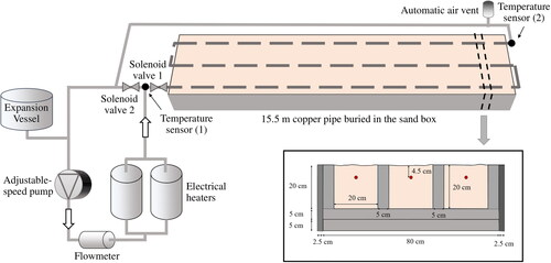
The fluid system consists of two pressurized hydraulic circuits separated by solenoid valves. One circuit represents the buried pipe section (right-hand circuit in Figure 4 and the other representing a heat source (left-hand circuit in Figure 4). The purpose of allowing separation into two circuits allows the fluid to be pre-heated to the desired step change temperature whilst leaving the test pipe section to be stabilized at the desired initial temperature. The solenoid valves allow the rapid introduction of warm fluid into the test section to provide a step change boundary condition. The main components of the heat source circuit and the buried pipe system in the sand are illustrated in Figures 5 and 6.

Fig. 5. A photograph from the heat source circuit of the experimental setup providing circulating hot water through the buried pipe.

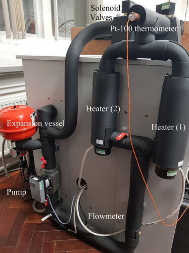
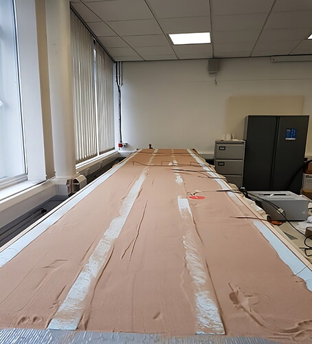
Fig. 6. A photograph of the buried pipe system in the sand.

Two fast-response PT100 RTD sensors (accuracy grade 1/10 DIN) are directly inserted into the buried pipe and used to measure the inlet and outlet temperatures of the test pipe section. The ambient temperature is measured with an adjacent type-T thermocouple. All the temperature sensors are calibrated using a calibration oil bath and a reference thermistor so that the uncertainty in the temperature measurements of the thermocouples and PT-100 RTD sensors have been estimated to be 0.167 K and 0.062 K, respectively.

The mass flow rate is measured by a vortex flowmeter with an uncertainty of less than two percent of the measured value. The variable speed pump is used to control and vary the flow rate in a way to be desirable for this study. A combination of the RTD flow temperature measurements and flowmeter data are used to calculate the instantaneous heat transfer rate at the pipe surface.

In order to measure the heat flux at the upper exposed (ground) surface, a direct measurement of flux is obtained using three self-calibrating heat flux sensors (HFP01SC by Hukseflux). This highly sensitive heat flux sensor incorporates the film heater to self-test and self-calibrate the sensor. These three self-calibrating heat flux sensors have been placed on the top of the sandboxes to measure the dynamic ground surface heat losses accurately. Since the diameter of the heat flux sensor is 8 cm, they are positioned in a way to cover all width of the sandbox, i.e. 20 cm. Therefore, by averaging the measured heat fluxes from the sensors, the average ground heat loss can be obtained.

Due to the importance of the thermal properties of the sand in modeling the buried pipe, these properties were measured independently using a needle probe dynamic thermal conductivity instrument before conducting the experiments. The measurements have been performed at the different locations of the sand over a period of a few hours to ensure that the properties were measured with the sand at the same density (compaction) as during the experiments. The range of results was analyzed to arrive at mean values with an uncertainty of 4.8%. These sand thermal properties, as well as those of the other materials used in the experiments, are presented in Table 1. Further details of instrument calibration and property measurements can be found in the associated thesis (Meibodi 2020).

Table 1. Thermal properties of the pipe materials and fluid.

Material	Thermal capacity (J/kg.K)	Thermal conductivity (W/m.k)	Density (kg/m^3)
Copper pipe	385	401	8960
Water	4181	0.61	998
Sand	667	0.173	1442

Using precise measurement instruments and conducting careful calibrations led to a reduced level of uncertainty in the experimental results. The compound uncertainty of the fluid heat balance and ground surface heat flux is estimated at 2.52% and 1.09%, respectively. Additionally, the uncertainty of the normalized pipeline heat flux and weighting factors is 2.58% and 4.42%, respectively. Meanwhile, the uncertainty of the normalized ground surface heat flux and weighting factors is 1.18% and 2.04%, respectively. The experimental results obtained from the experiments along with their corresponding uncertainties will be presented and discussed in Section 5.

Two main experiments have been conducted to obtain the step response heat flux of the surface of the buried pipe system. In these experiments, a step change is applied to each surface’s boundary temperature, and the heat transfer rate of both surfaces is measured and collected simultaneously. It should be noted that in the process of derivation of weighting factor values, the step response heat flux series corresponding to the step change from zero to one is required. Therefore, the measured step response flux series needs to be normalized in a way that can be expressed as equivalent to a unit step change. This is carried out by normalizing the series with respect to the experimental conditions of each experiment, as follows: (9) $$Q_{\text{normalized}}=Q/\left(T_{\text{step}\text{change}}-T_{\text{initial}}\right)$$(9) where T_{step change} and T_initial are the step change temperature imposed to the surface and initial temperature of the system, respectively. Normalizing the heat transfer rates also results in the obtained heat flux series becoming independent of the temperature conditions of the experiments. This also allows the operating temperature range to be increased relative to the measurement uncertainties in order to reduce their significance as far as possible. The details of the procedure of the experiments are described in the following.

To impose a step change to the buried pipe, a temperature step change was applied to the inlet temperature of the test section. To achieve this the water is circulated in the heat source circuit to be preheated by passing through the electric heaters, while the buried pipe section is naturally stabilized at ambient room temperature. When conditions are stabilized, the step change in inlet temperature is imposed by opening the solenoid valve between the two circuits. This allows the hot water to flow through the buried pipe at the set inlet temperature and mass flow rate. To maintain the inlet temperature constant, a closed-loop feedback controller is used to modulate heat input according to the inlet temperature. The inlet and outlet temperatures of the buried pipe section, as well as the flow rate and the ground heat fluxes, are recorded at the given time step during the experiments until the steady-state conditions are approached: almost 42 h.

To apply a step change to the ground surface, one approach would be for the lab temperature to undergo a step change, while the sand and water flow are stabilized. This is not practical, however. Rather, the direction of heat flow is reversed. In this approach, the sand and pipe section is pre-heated to achieve a uniform initial temperature elevated above the lab ambient temperature. This is done using the pipe as a heater but adding additional insulation to the top of the sand temporarily and so enabling isothermal conditions to be reached. A step change is then achieved by rapidly removing the upper insulation and instantly exposing the upper surface to the ambient conditions. The pipe fluid temperature is maintained at the initial temperature during the whole experiment. The lab temperature was monitored and found to vary by only 0.9 K during the whole 42 h of the experiment and so exposing the heated box to the lab in this way seems to closely approach a step response. The details of this step-change process are described below.

Temporary insulation was achieved by using a combination of flexible foam insulation fixed to rigid foam insulation and placed on top of the sand layer. This arrangement allowed the elimination of any air pockets and air leakage over the sand surface. Several sandbags were put on top of the insulation boards to ensure good contact during the pre-heating phase.

The temperature variations in different points of the sand were monitored during the pre-heating process to check conditions approximating a stable isothermal condition were reached. Subsequently rapidly removing the upper insulation allows the reversed step change to start and data recorded until steady conditions were approached.

The fluid flow conditions in both experiments needed to be turbulent and constant in order to represent the constant convection coefficient conditions assumed in the derivation of the weighting factors. Considering the pump characteristics and pressure drop in the pipeline, the pump speed was set to achieve turbulent flow conditions but also low enough to achieve a total temperature difference high enough relative to the uncertainty in the temperature measurements.

The details of the conditions of both experiments are presented in Table 2. The difference in the water velocity in the experiments (0.027 m/s) results in a small difference between the Reynolds numbers (550). This leads to approximately 5% difference in the calculated pipe convective heat transfer coefficients. However, since the superposition of both admittive conductances (K₁, K₂) and transmittive conductance (K₁₂) are used in the DTN calculation, the impact on the overall uncertainly is much smaller. The experimental results and numerical outputs are discussed in the following sections.

Table 2. Experimental conditions of the experiments on the buried pipe systems.

Test case	Water velocity (m/s)	Convective coefficient (W/m^2 K)	Step change temperature difference	Average lab temperature (C^o)	Initial temperature (C^o)
Case (1)(1) $$\begin{array}{c}{Q}_1\left(t\right)=\mathrm{ }{Q}_{1a}\left(t\right)+Q_{12}\left(t\right)\\ Q_2\left(t\right)=\mathrm{ }{Q}_{2a}\left(t\right)+Q_{21}\left(t\right)\end{array}$$(1) -Buried pipe surface step change	0.246	1551	21.8	16.2	16.0
Case (2)(2) $$\begin{array}{c}{Q}_1\left(t\right)=\mathrm{ }{K}_1\mathrm{ }\left[T_1\left(t\right)-\overline{T_{1a}}\left(t\right)\right]+\mathrm{ }{K}_{12}\mathrm{ }\left[\overline{T_{12}}\left(t\right)-\overline{T_{21}}\left(t\right)\right]\\ Q_2\left(t\right)=\mathrm{ }{K}_2\mathrm{ }\left[T_2\left(t\right)-\overline{T_{2a}}\left(t\right)\right]+\mathrm{ }{K}_{12}\mathrm{ }\left[\overline{T_{21}}\left(t\right)-\overline{T_{12}}\left(t\right)\right]\end{array}$$(2) - Ground surface step change	0.273	1645	21.9	16.1	38.0

Results and discussion

Measured step responses

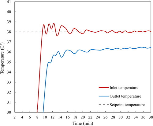
In order to ensure consistent experimental results, it is essential to be able to apply a precise temperature step change to both the pipeline and ground surfaces. This requires careful control of the heaters in the experimental setup, particularly after solenoid valves are opened, to make sure the inlet temperature of the pipeline remains constant throughout the experiments after imposing the step change. To achieve that, a closed-loop feedback controller is employed to regulate the power of the heaters according to the difference between the inlet temperature and the set-point temperature at any given moment. More details on controlling the heaters can be found in the associated thesis. The resulting inlet and outlet temperatures of the pipeline for test case 1 are displayed in Figure 7.

Fig. 7. Variations of the inlet and outlet temperatures of the pipeline controlled by close-loop feedback controller at the early stage of applying the step change of the buried pipeline.

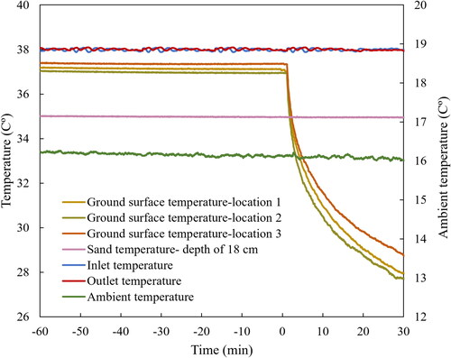
As described in Section 4, a step change was introduced to the ground surface by pre-heating the sand and pipe section until a stable condition was achieved and subsequently, removing the upper insulation to create a reverse step change. To determine if stable conditions were reached, three thermocouples were placed on different locations of the ground surface and one was buried 18 cm into the sand and their temperature variations were carefully monitored. Having ensured the condition is stable, the step change is imposed by rapidly removing the insulation. The temperature variations of the ground surface and the sand as well as the inlet, outlet and ambient temperature are shown in Figure 8. It should be noted that the negative time indicates the initial conditions before the moment of applying the ground surface step change.

Fig. 8. Fluctuations in temperature of the ground surface, sand, inlet, outlet, and ambient temperatures before and after applying the ground surface step change.

Having determined the pipeline and ground surface step response heat flux data from both experiments, the admittive and transmittive heat flux components can be obtained. To that end, the step response data needs to be expressed as equivalent to a unit temperature step change (0–1). Hence, all heat flux data obtained in the experiments are divided by the temperature differences between the step change temperature and initial temperature of the system based on Equation 9(9) $$Q_{\text{normalized}}=Q/\left(T_{\text{step}\text{change}}-T_{\text{initial}}\right)$$(9) . This also allows comparison of results from different experiments on a similar basis.

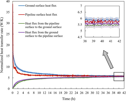
Figure 9 illustrates the normalized step change heat fluxes obtained from two experiments from the moment of applying the boundary step change until the system approaches steady-state conditions. It can be seen that both normalized heat fluxes from the ground surface to the pipeline surface and vice versa obtained from each test are very similar. These values correspond to that at the surface at ambient conditions during the test (i.e. zero temperature when normalized) and should be theoretically the same since they represent the transmittive heat transfer process from one surface to another depending only on the thermal properties of the materials and the geometric arrangement. Moreover, it can be seen as time proceeds all heat fluxes approach a very similar value, i.e. the steady-state conductance. This demonstrates the consistency of the experiments.

Fig. 9. Variations of the normalized heat flux step responses of the pipeline and ground surface.

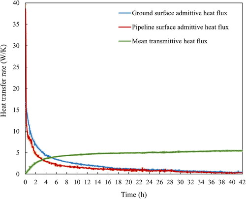
Figure 10 shows the normalized admittive and mean transmittive heat fluxes calculated based on the normalized step response heat flux data determined from both experiments. At the beginning of applying the step change to the boundary temperatures, the admittive heat fluxes are maximum, i.e. equal to the surface conductances, while the transmittive heat flux is zero. As the buried pipeline system approaches the steady-state conditions, the admittive heat fluxes approach zero, whereas the transmittive component becomes close to the steady-state conductance. Acknowledging some small difference may be attributable to the slightly different flow rates, the mean of the transmitted fluxes (Figure 9) is shown as the transmittive fluxes in Figure 10.

Fig. 10. The normalized admittive and transmittive step response heat fluxes for the buried pipeline system.

One of the main objectives of this research was to experimentally investigate the validity of the DTN approach. To this end, the step response heat flux data determined from the pipeline and ground surfaces from both experiments are used for the calculation of the weighting factor series. These weighting factor series are compared with that calculated from the two-dimensional version of the finite volume model (see Section 3.2.2) as a computationally convenient way of numerically deriving of weight factor series.

One of the objectives has been to implement the weighting factors obtained both numerically (from the 2D model) and experimentally (from the measured fluxes) into the DTN model to evaluate the suitability of the DTN model in representing the dynamic behavior of the buried pipeline system. The simulation results from the DTN model are compared with the experimental data in terms of the prediction of the dynamic heat losses from the ground and pipeline surfaces.

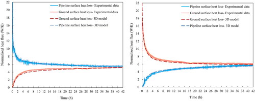
In all the comparisons made with experimental data in the following, the detailed three-dimensional conjugate heat transfer model is used in comparisons of the proposed DTN model and with the 2D finite volume model in terms of accuracy and computational expense. Figure 11 displays the normalized step response fluxes resulting from imposing the step change on the boundary temperature from both the experimental data and the detailed 3D model at the pipeline and at the ground surface. It can be observed there is a good level of agreement between the 3D model results and experimental data.

Fig. 11. The normalized heat fluxes of step changes at the ground surface (left) and the pipeline surfaces (right) obtained from the experimental data and the 3D conjugate heat transfer model.

Weighting factors derivation using the FVM

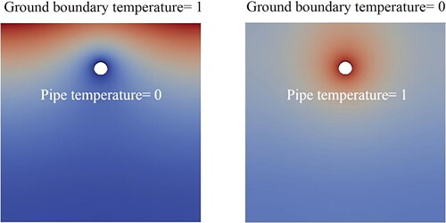
To derive the weighting factor series using a 2D finite volume model of conduction heat transfer, the boundary conditions need to be convective with constant heat transfer coefficients in order to have consistent DTN model calculation. However, once the weighting factors are determined, the heat transfer coefficient of the surfaces can be adjusted in the DTN model for different fluid flow rates and boundary conditions. Therefore, it is necessary to define suitable heat transfer coefficients for each surface for the calculation of the weighting factor series. To this end, the heat transfer coefficient at the inner surface of the pipeline is chosen from the mean values determined based on the well-known Gnielinski’s correlation from the experiments (presented in Table 2) and calculated as 1598 W/m²K. This was found to be consistent with the full conjugate heat transfer calculations. The ground surface heat transfer coefficient is estimated to 8.2 W/m²K based on the measured ground surface temperatures and heat fluxes along with the lab temperatures. These values as well as the thermal properties of the pipeline and the sand measured in this work are prescribed in the finite volume model (2D models) to simulate the transient heat transfer of the buried pipeline system. Figure 12 shows the temperature distribution of the ground having undergone the unit step change at the pipeline and ground surfaces.

Fig. 12. Temperature distributions in the sand box after 1000 s from imposing the unit step change to the ground surface (left), and the pipe surface (right) calculated using the 2D numerical model.

Weighting factor derivation using experimental data

For the derivation of the weighting factors, unit step response fluxes (shown in Figure 9) need to be applied in the calculation. The comparison between the unit step response dynamic fluxes normalized by the corresponding conductances from the 2D model and the experiments over the entire duration of the tests are illustrated in Figure 13. The admittive (Q_1a, Q_2a) and the transmittive fluxes (Q₁₂) are shown normalized by the corresponding thermal conductances (K₁, K₂, K₁₂). The thermal conductances (K₁, K₂) are calculated based on maximum admittive fluxes (equal to surface area multiplied by the surface heat transfer coefficient), and the thermal conductance (K₁₂) is obtained from the steady-state transmittive flux to the unit temperature difference, i.e. values at the end of the test.

Fig. 13. The buried pipe admittive and transmittive response fluxes obtained from the 2D model and the experiments normalized by the corresponding conductances.

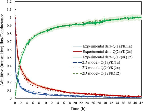
It can be also observed that the pipeline admittive flux (Q_1a) and the ground surface admittive flux (Q_2a) diminish at the beginning and approach zero at the steady-state condition. However, the rate of the decrease of the pipeline admittive flux is higher than the ground admittive flux, as the pipeline admittive flux drops 10% of the maximum value after 4.2 h compared with 13.5 h for the ground admittive flux. Also, the admittive fluxes (Q_1a, Q_2a) have fallen 2% of their maximum after 29.8, 38.1 h, respectively. In addition, it can be observed that the transmittive flux increases to 80% of the steady-state value after 7.5 h and then increases more slowly before reaching its final value. This flux reaches 99% of its steady-state values after 36.1 h.

These heat flux time series data are used to derive the weighting factors by applying Equation 7(7) $$\begin{array}{c}{\kappa }_{ia,p}=\frac{\overline{Q_{ia}}\left(\rho \mathrm{\Delta }t\text{-}\mathrm{\Delta }t\right)-\overline{Q_{ia}}\left(\rho \mathrm{\Delta }t\right)}{\overline{K_i}}\\ {\kappa }_{i\mathrm{j},p}=\frac{\overline{Q_{\mathrm{ij}}}\left(\rho \mathrm{\Delta }t\text{-}\mathrm{\Delta }t\right)-\overline{Q_{\mathrm{ij}}}\left(\rho \mathrm{\Delta }t\right)}{\overline{K_{i\mathrm{j}}}}\end{array}$$(7) . The weighting factor series derived from the numerical model and experimental data are later used as input parameters in the DTN model calculation to predict the pipeline and ground surface heat transfer rates and compared with the measured data.

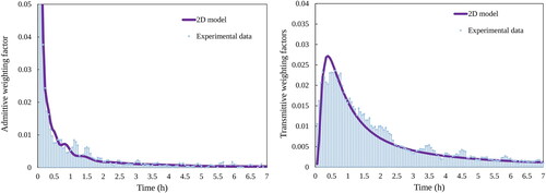
Figure 14 displays the corresponding weighting factors for the buried pipeline admittive and transmittive fluxes determined both numerically and experimentally over the first seven hours of the tests according to Equation 7(7) $$\begin{array}{c}{\kappa }_{ia,p}=\frac{\overline{Q_{ia}}\left(\rho \mathrm{\Delta }t\text{-}\mathrm{\Delta }t\right)-\overline{Q_{ia}}\left(\rho \mathrm{\Delta }t\right)}{\overline{K_i}}\\ {\kappa }_{i\mathrm{j},p}=\frac{\overline{Q_{\mathrm{ij}}}\left(\rho \mathrm{\Delta }t\text{-}\mathrm{\Delta }t\right)-\overline{Q_{\mathrm{ij}}}\left(\rho \mathrm{\Delta }t\right)}{\overline{K_{i\mathrm{j}}}}\end{array}$$(7) . It can be seen that after 7 h, the weighting factors corresponding to the pipeline admittive and transmittive flux diminish to below 0.0004 and 0.0271 (3% of the maximum value), respectively.

Fig. 14. The buried pipeline admittive (left) and transmittive (right) weighting factors calculated based on the corresponding the step response fluxes from both the experimental measurement and the 2D model.

A good match between the weighting factor series derived from experimental data and numerical model shows the verification of the DTN approach, as for the first time the weighting factor series derived purely from the experimental data. The weighting factor series are used in the DTN model for further investigation of ability of the models in prediction of dynamic heat losses of the buried pipeline system.

The discrete weighting factor series derived experimentally can be observed (Figure 14) to be less smooth than the variation in those calculated numerically. This is most likely due to the higher frequency variations (noise) in the experimental data. However, there are larger fluctuations in the discretized weighting factors derived from the experimental data. The accuracy in the steady-state is a function of the summation of the weighting factors, i.e. the area under the curve. In this case the variations tend to cancel out and aren’t a great concern. The effects of the added fluctuations in the weighting factors obtained from the experimental measurement on the output of the DTN model are discussed in the following Sections.

Ground transient heat transfer

The predicted ground surface heat transfer rates are compared with the measured values when imposing a step change to the pipeline inlet temperature, in Figure 15. The magnitude of the discrepancies between measured and predicted ground surface heat losses by the numerical models are shown Figure 16. In these figures, the DTN results using weighting factors derived from the 2D FVM model are denoted Numerical kappa.

Fig. 15. Measured and calculated ground boundary heat transfer using the 3D FVM model and the DTN model with both forms of weighting factor data.

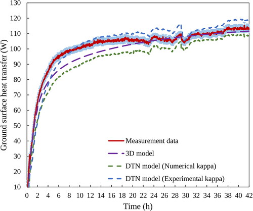
Fig. 16. Differences between the measured and calculated ground boundary heat transfer.

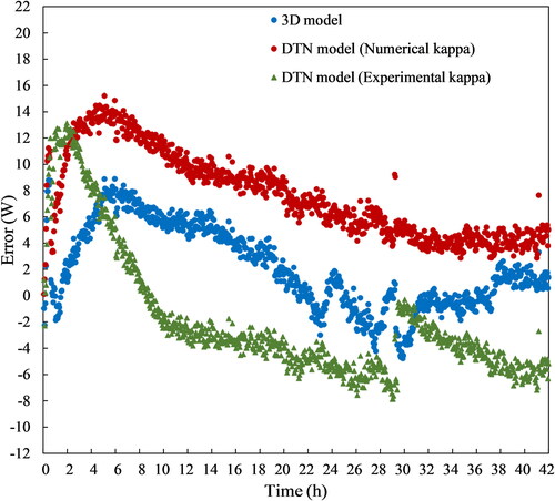
It can be seen (Figure 16) that the difference between the heat fluxes predicted by the models mostly lies below 7.5% of the steady-state value. As time increases, the difference relative to the measured heat transfer becomes smaller for all models so that the final values show differences less than 5% in magnitude.

Ground heat transfer rates are partly dependent on lab conditions and these could not be controlled ideally over the whole period. A maximum of 0.9 K variation was noted earlier. Some particular fluctuations are observable between 22 and 30 h. These do not have a significant effect on the heat transfer overall. However, the variation in lab temperature is reflected in the results of the DTN models as they are driven by time varying boundary conditions accordingly.

A potential advantage of using experimental heat flux data to derive weighting factors is that separate measurements or estimates of thermal properties do not need to be considered: these are implicit to the overall heat fluxes. In contrast, thermal properties have to be considered explicitly in a numerical model and some uncertainties arise from this. This seems to be reflected in the results shown in Figure 16 where in the period 4–20 h there is a better match with measured values using the experimentally derived weighting factors. In particular, the numerical values show slower changes in ground heat flux. In this period, thermal diffusion (or heat capacity and density product) is significantwhereas longer-term conductivity becomes more significant as steady-state conditions are approached. This suggests that the value of thermal diffusivity used in the numerical models may be a little high.

Pipe transient heat transfer

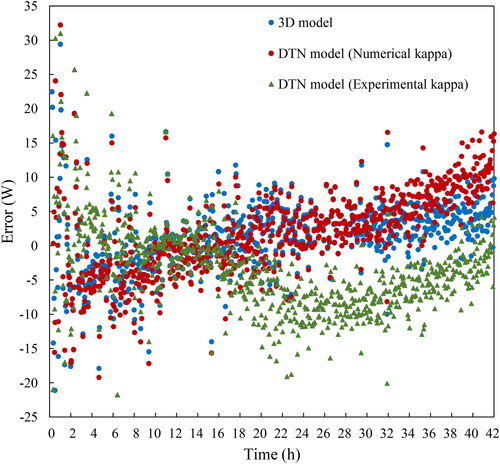
Figure 17 illustrates the comparisons between the predicted pipeline heat transfer and measured values when imposing the step change in inlet temperature on the pipeline. Some deviations from the step response flux trend are observed (16–22 h) in the heat loss prediction by the DTN model that uses the weighting factors determined experimentally. This is most likely to be a result of some weighting factors being unduly influenced by high frequency variations (noise) in the experimental data. This was noted in the discussion of the data in Figure 14. The differences between the measured and simulated pipe heat transfer rates are illustrated in Figure 18. These differences tend to be largest at the early stages of the step when rates of change and temperature gradients are at their largest. It can also be seen that there is greater scatter in the data for the pipe heat transfer rate than that of the ground (Figure 16). This again reflects the high frequency variations in the experimental heat transfer rate data (Figure 17). There are probably greater fluctuations in this data compared to that of the ground surface due to these fluxes being determined from the fluid heat balance using three measurements (flow rate and two temperatures) rather than a single heat flux sensor in the latter case.

Fig. 17. Measured and calculated buried pipe boundary heat losses using the 3D FVM model and the DTN model with both forms of weighting factor data.

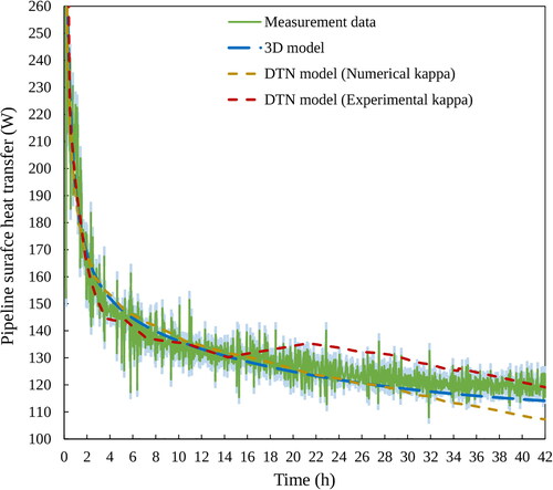
Fig. 18. Differences between the measured and calculated buried pipe boundary heat transfer.

Overall uncertainty assessment

A further useful metric of the differences between the models and the experimental data is the Root Mean Square Error (RMSE) based on the data over the duration of the test or simulation. This is calculated according to Equation 10(10) $$\mathit{RMSE}=\sqrt{\frac{1}{n}{\sum }_{i=1}^n{\left(Y_{\text{simulation,i}}-Y_{\text{experimental data},i}\right)}^2}$$(10) . (10) $$\mathit{RMSE}=\sqrt{\frac{1}{n}{\sum }_{i=1}^n{\left(Y_{\text{simulation,i}}-Y_{\text{experimental data},i}\right)}^2}$$(10)

In this case, Y is the pipe or ground heat flux. Figure 19 displays a comparison of RMSE between the measured and predicted heat losses from the pipeline and ground surfaces during the entire test time, i.e. 42 h. The error bars indicate the magnitude of the uncertainty in the heat flux measurements. The results for each form of calculation of the step change have RMSE values for the boundary fluxes that are less than 13 W. This is viewed an acceptable level of accuracy for engineering design and analysis purposes.

Fig. 19. RMSE between the calculated heat losses from the pipe and ground surfaces and experimental data for the buried pipe step-change test.

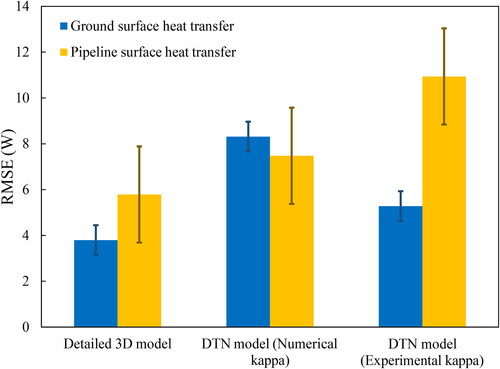
The RMSE values are highest for the prediction of pipe heat transfer using the DTN model with weighting factors derived from the experimental data directly. This is thought to be a consequence of the impact of the high frequency fluctuations in the flux data having some impact on the discrete weighting factors. This might be improved but the purpose of applying the experimental data in this way was to demonstrate the validity of the DTN approach for one particular case. The intention is that a numerical approach is applied for study of particular engineering designs as it can be readily adapted to each geometry and set of thermal properties.

Computational efficiency

Modeling heat flux responses of the buried pipes in this research has been carried out using two main numerical models: the three-dimensional model and the DTN model (using weighting factors derived numerically and experimentally). In the three-dimensional conjugate heat transfer model, all the governing equations for both fluid and solid domains require to be solved resulting in a very long calculation time. To make the calculation efficient, the solver used in modeling the 3D model was adapted to use increasing time steps, i.e. from 0.001 s to a few seconds. However, even after applying this approach, the calculation time required for the simulation of the 3D buried pipe system over the 42 h corresponding to the experiment is very high. The simulation of the buried pipe using 20 parallel processors (Intel(R) CPU E5-2699 @ 2.30 GHz) took more than three days.

The computational cost of the DTN approach can be calculated based on three main calculation stages: (i) the step response heat flux calculation, (ii) weighting factors derivation, and (iii) the DTN simulation run-time. Since the first two processes require to be performed just once, their calculation time is often negligible compared with the primary DTN simulation time, i.e. reading the weighting factor data and solving the heat balance equations for extensive time series.

A preferred approach to obtaining the step response heat flux series of the buried pipe system, the 2D FVM conduction heat transfer solver is used, exploiting the same increasing time steps approach as the 3D model. Since the model only needs to deal with the two-dimensional transient conduction heat transfer in the solid domain with the mixed boundary conditions, the simulation time is considerably lower than the 3D model: a couple of minutes for the buried pipe using one processor (Intel(R) CPU E5-2699 @ 2.30 GHz).

The time required for obtaining the step response heat flux series from experiments depends on the time needed for the system to reach the steady-state conditions: 42 h for the buried pipe system in the experiments. Both sets of step response heat flux data from the 2D model and experiments are further used to derive the weighting factor series. These can be used for any conditions as long as the geometry and set of thermal properties of the system do not vary. Typical simulation inputs would be inlet fluid temperatures and flow rates along with ambient temperatures.

The computational time required to simulate the experimental buried pipe system has been compared between the numerical models for the buried pipe step change test. The results are enumerated in Table 3. It can be observed that the DTN model using both numerical and experimental weighting factors is more than five orders of magnitude more computationally efficient than the 3D conjugate heat transfer model. The computational efficiency of the DTN model is a considerable advantage, particularly for the simulation of more extensive time series and complex buried pipe configurations, e.g. DHC pipelines.

Table 3. Comparison between the calculation time required for the numerical models to modeling the buried pipe system and their accuracy.

Numerical models	Simulation run-time (s)	RMSE between the calculation ground surface heat losses and experimental data (%)
3D FVM	296000	3.39
2D FVM	193	–
DTN model (Weighting factors derived experimentally)	5.4	5.52
DTN model (Weighting factors derived numerically)	3.9	7.49

Moreover, the DTN model using weighting factors derived experimentally can be seen to have a little higher calculation time: less than two seconds. This is because the model requires dealing with a higher number of experimental heat flux input data for the derivation of the weighting factors compared with that of obtained from the 2D model. It should be noted the DTN simulation running time is the same for both approaches of obtaining weighting factors, since the DTN model uses the weighting factor series as input parameters.

Conclusions

The Dynamic Thermal Network (DTN) approach, as a response factor method, offers a number of significant advantages over conventional numerical models, which makes it well-suited for dynamic thermal modeling of any complex three-dimensional with time-varying boundary conditions. In this study, the DTN approach to the calculation of conduction heat transfer time series has been evaluated experimentally in the case of ground material with an embedded pipe.

A new experimental facility has been implemented to allow the application of step changes in operating temperature and measuring heat fluxes at the pipe and the ground surfaces. This is based on a reduced scale district heating pipe buried in a sand material to represent the ground. Testing has been possible over a period where the heat transfer rate approaches a steady state. This is sufficient to provide validation data for comparisons with numerical models of transient heat transfer.

The derivation of weighting factors in the DTN approach is agnostic with regard to the origin of the step response heat flux data. Consequently, it has been possible to demonstrate how experimental heat flux data could be used to calculate weighting factors. This has the advantage of not requiring thermal property or detailed geometry data. This has been successful in showing the DTN calculations of the test are consistent with the experimental data. It has also highlighted some of the challenges in applying step boundary conditions and measuring relatively small heat fluxes.

For practical application in design studies, it is intended that weighting factors are derived numerically for most cases. Two forms of the Finite Volume Model have been implemented to assess this approach. A three-dimensional model of conjugate heat transfer (both fluid motion and conduction heat transfer) representing the experimental geometry and properties have been implemented. This model was used to capture all potential heat transfer effects influencing pipe and ground surface heat fluxes. The results have shown the model capable of representing experimental conditions with a very good level of accuracy. This model has subsequently been used as a reference model in comparison with DTN calculations with weighting factors calculated using a simpler 2D model and a further set of weighting factors derived from the experimental data directly.

Using weighting factor data derived from experimental heat flux data has proved to be possible. However, there are no particular benefits in terms of accuracy compared to the application of numerical models. Modeling the step response test using a 2D model is a simplification of the 3D model both in terms of geometry and also in that only conduction through the solid parts of the domain is modeled explicitly. Comparing 2D and 3D model results have allowed the significance of these simplifications to be assessed. It has been possible to show the differences in the calculated fluxes have been shown to be relatively small.

The fluid in the pipe can be represented by the choice of a suitable convection coefficient at the pipe wall. This simplification does not seem to be significant given a suitable empirical convection correlation. The other main question regarding the acceptability of a 2D model is whether longitudinal effects are significant, e.g. near the entrance to the pipe. Such effects have been shown to be insignificant when comparing the overall RMSE in the prediction of pipe and ground fluxes given the proportions of the buried pipeline. As the 2D model is more than an order of magnitude less demanding in computational effort, it seems a perfectly acceptable way to calculate weighting factors for DTN models of buried pipes.

Each of the modeling approaches tested in this work was able to predict pipe and ground heat fluxes with RMSE of less than 10\%. The method recommended for further application employs a 2D numerical model to derive the weighting factors for a DTN model. This was shown to have RMSE for both fluxes at approximately 8%. This should be acceptable for most engineering design and analysis tasks. Once the DTN weighting factors have been calculated, the final DTN simulation has been shown to be several orders of magnitude quicker than the finite volume method simulations.

The initial application in mind has been the prediction of ground and pipe heat transfer in heating and cooling networks. The DTN approach reported here is best suited to deal with long timescale ground heat transfer effects and will be combined with a further model of short term response (Meibodi and Rees 2020) to form a heat network model and this is to be reported elsewhere. A number of other applications have similarity to that studied here in terms of dynamic heat transfer in the ground with an embedded linear heat source/sink. We suggest the DTN approach could accordingly be used, for example, to study horizontal ground heat exchanger systems, buried cable heat transfer, oil pipelines, earth ducts, or heat transfer in infrastructure tunnels.

Nomenclature
$A$	=	surface area (m2)
$C$	=	specific heat capacity (kJ/kg.K)
$\Delta \mathrm{t}$	=	time step size (s)
$\Delta \mathrm{x}$	=	cell size (m)
$\mathrm{h}$	=	heat transfer coefficient (W/ m2.K)
$K$	=	conductance (W/K)
$\overline{K}$	=	modified conductance (W/K)
$L$	=	layer thickness (m)
$N$	=	number of surfaces
P	=	period (s)
$Q$	=	heat transfer rate (W)
$\overline{Q}$	=	average heat transfer rate (W)
$\mathrm{R}$	=	thermal resistance (K/W)
$r$	=	pipe radius (m)
$T$	=	temperature (oC)
$\overline{T}$	=	weighted average temperature (oC)
$t$	=	time (s)
BHE	=	borehole heat exchanger
DHC	=	district heating and cooling
DTN	=	dynamic thermal network
FEM	=	finite element method
FHE	=	foundation heat exchanger
FVM	=	finite volume method
GHE	=	ground heat exchanger
GSHP	=	ground source heat pump
RTD	=	resistance temperature detectors
UTES	=	underground thermal energy storage

Greek letters
$\kappa$	=	weighting function
$\rho$	=	density
$\tau$	=	time (integration variable) (s)

Subscripts/Superscripts
i, j	=	surface number
n	=	time step index
a	=	admittive
t	=	transmittive
p	=	weighting factor index

Disclosure statement

No potential conflict of interest was reported by the authors.

References

- Arabkoohsar, A., M. Khosravi, and A. S. Alsagri. 2019. CFD analysis of triple-pipes for a district heating system with two simultaneous supply temperatures. International Journal of Heat and Mass Transfer 141:432–43. doi:10.1016/j.ijheatmasstransfer.2019.06.101.
- Bau, H. H., and S. S. Sadhai. 1982. Heat losses from a fluid flowing in a buried pipe. International Journal of Heat and Mass Transfer 25 (11):1621–9. doi:10.1016/0017-9310(82)90141-7.
- Bennet, J., C. Johan, and Hellström, G. 1987. Multipole method to compute the conductive heat flows to and between pipes in a composite cylinder.
- Bøhm, B. 2000. On transient heat losses from buried district heating pipes. International Journal of Energy Research 24 (15):1311–34.
- Chen, L., W. Yu, Y. Lu, P. Wu, and F. Han. 2021. Characteristics of heat fluxes of an oil pipeline armed with thermosyphons in permafrost regions. Applied Thermal Engineering 190:116694. doi:10.1016/j.applthermaleng.2021.116694.
- Claesson, J. 2002. Dynamic Thermal Networks. Outlines of a General Theory. Proceedings of the 6th Symposium on Building Physics in the Nordic Countries Trondheim. Norway, Trondheim: 47–54.
- Claesson, J. 2003. Dynamic thermal networks: A methodology to account for timedependent heat conduction. Proceedings of the Second International Conference on Research in Building Physics. Leuven, Belgium: 407–15.
- Dahash, A., F. Ochs, A. Tosatto, and W. Streicher. 2020. Toward efficient numerical modeling and analysis of large-scale thermal energy storage for renewable district heating. Applied Energy 279:115840. doi:10.1016/j.apenergy.2020.115840.
- Dalla Rosa, A., H. Li, and S. Svendsen. 2011. Method for optimal design of pipes for low-energy district heating, with focus on heat losses. Energy 36 (5):2407–18. doi:10.1016/j.energy.2011.01.024.
- Dalla Rosa, A., H. Li, and S. Svendsen. 2013. Modeling transient heat transfer in small-size twin pipes for end-user connections to low-energy district heating networks. Heat Transfer Engineering 34 (4):372–84. doi:10.1080/01457632.2013.717048.
- Danielewicz, J., B. Śniechowska, M. A. Sayegh, N. Fidorów, and H. Jouhara. 2016. Three-dimensional numerical model of heat losses from district heating network pre-insulated pipes buried in the ground. Energy 108:172–84. doi:10.1016/j.energy.2015.07.012.
- Dénarié, A., M. Aprile, and M. Motta. 2019. Heat transmission over long pipes: New model for fast and accurate district heating simulations. Energy 166:267–76. doi:10.1016/j.energy.2018.09.186.
- Eggels, J. G. M., F. Unger, M. H. Weiss, J. Westerweel, R. J. Adrian, R. Friedrich, and F. T. M. Nieuwstadt. 1994. Fully developed turbulent pipe flow: A comparison between direct numerical simulation and experiment. Journal of Fluid Mechanics 268:175–210. doi:10.1017/S002211209400131X.
- Fan, D., S. Rees, and J. Spitler. 2013. A dynamic thermal network approach to the modelling of foundation heat exchangers. Journal of Building Performance Simulation 6 (2):81–97. doi:10.1080/19401493.2012.696144.
- Gabrielaitiene, I., B. Bøhm, and B. Sunden. 2008. Evaluation of approaches for modeling temperature wave propagation in district heating pipelines. Heat Transfer Engineering 29 (1):45–56. doi:10.1080/01457630701677130.
- Gnielinski, V. 1976. New equations for heat and mass transfer in turbulent pipe and channel flow. International Chemical Engineering 16 (2):359–68.
- Guelpa, E. 2020. Impact of network modelling in the analysis of district heating systems. Energy 213:118393. doi:10.1016/j.energy.2020.118393.
- Guelpa, E., and V. Verda. 2019. Thermal energy storage in district heating and cooling systems: A review. Applied Energy 252:113474. doi:10.1016/j.apenergy.2019.113474.
- Khosravi, M., and A. Arabkoohsar. 2019. Thermal-hydraulic performance analysis of twin-pipes for various future district heating schemes. Energies 12 (7):1299. DOI: 10.3390/en12071299.
- Li, M., T. S. Khan, E. Al-Hajri, and Z. H. Ayub. 2016. Single phase heat transfer and pressure drop analysis of a dimpled enhanced tube. Applied Thermal Engineering 101:38–46. doi:10.1016/j.applthermaleng.2016.03.042.
- Lund, H., P. A. Østergaard, M. Chang, S. Werner, S. Svendsen, P. Sorknæs, J. E. Thorsen, F. Hvelplund, B. O. G. Mortensen, B. V. Mathiesen, et al. 2018. The status of 4th generation district heating: Research and results. Energy 164:147–59. doi:10.1016/j.energy.2018.08.206.
- Meibodi, S. 2020. Modelling dynamic thermal responses of pipelines in thermal energy networks. PhD thesis, University of Leeds, UK.
- Meibodi, S. S., and F. Loveridge. 2022. The future role of energy geostructures in fifth generation district heating and cooling networks. Energy 240:122481. doi:10.1016/j.energy.2021.122481.
- Meibodi, S. S., and S. Rees. 2020. Dynamic thermal response modelling of turbulent fluid flow through pipelines with heat losses. International Journal of Heat and Mass Transfer 151:119440. doi:10.1016/j.ijheatmasstransfer.2020.119440.
- Naicker, S. S., and S. J. Rees. 2018. Performance analysis of a large geothermal heating and cooling system. Renewable Energy.122:429–42. doi:10.1016/j.renene.2018.01.099.
- Ocłoń, P., P. Cisek, M. Rerak, D. Taler, R. V. Rao, A. Vallati, and M. Pilarczyk. 2018. Thermal performance optimization of the underground power cable system by using a modified Jaya algorithm. International Journal of Thermal Sciences 123:162–80. doi:10.1016/j.ijthermalsci.2017.09.015.
- Peng, C., N. Geneva, Z. Guo, and L.-P. Wang. 2018. Direct numerical simulation of turbulent pipe flow using the lattice Boltzmann method. Journal of Computational Physics 357:16–42. doi:10.1016/j.jcp.2017.11.040.
- Rees, S., and G. Van Lysebetten. 2020. A response factor approach to modelling long-term thermal behaviour of energy piles. Computers and Geotechnics 120:103424. doi:10.1016/j.compgeo.2019.103424.
- Rees, S. J. 2015. An extended two-dimensional borehole heat exchanger model for simulation of short and medium timescale thermal response. Renewable Energy.83:518–26. doi:10.1016/j.renene.2015.05.004.
- Rees, S. J. 2016. 1 – An introduction to ground-source heat pump technology. In Advances in Ground-Source Heat Pump Systems, ed. S. J. Rees, 1–25. London, UK: Woodhead Publishing.
- Rees, S. J., and D. Fan. 2013. A numerical implementation of the dynamic thermal network method for long time series simulation of conduction in multi-dimensional non-homogeneous solids. International Journal of Heat and Mass Transfer 61:475–89. doi:10.1016/j.ijheatmasstransfer.2013.02.016.
- Shafagh, I., S. Rees, I. Urra Mardaras, M. Curto Janó, and M. Polo Carbayo. 2020. A model of a diaphragm wall ground heat exchanger. Energies 13 (2):300. DOI: 10.3390/en13020300.
- Shafagh, I., and S. J. Rees. 2018. Foundation wall heat exchanger model and validation study. IGSHPA research track. Stockholm 49. doi:10.22488/okstate.18.000045.
- Taler, D., and J. Taler. 2017. Simple heat transfer correlations for turbulent tube flow. E3S Web of Conferences 13:02008. doi:10.1051/e3sconf/20171302008.
- Thiyagarajan, R., and M. M. Yovanovich. 1974. Thermal resistance of a buried cylinder with constant flux boundary condition. Journal of Heat Transfer 96 (2):249–50. doi:10.1115/1.3450174.
- van der Heijde, B., A. Aertgeerts, and L. Helsen. 2017. Modelling steady-state thermal behaviour of double thermal network pipes. International Journal of Thermal Sciences 117:316–327. doi:10.1016/j.ijthermalsci.2017.03.026.
- Vasilyev, G. P., N. V. Peskov, and T. M. Lysak. 2022. Heat balance model for long-term prediction of the average temperature in a subway tunnel and surrounding soil. International Journal of Thermal Sciences 172:107344. doi:10.1016/j.ijthermalsci.2021.107344.
- Weller, H. G., G. Tabor, H. Jasak, and C. Fureby. 1998. A tensorial approach to computational continuum mechanics using object-oriented techniques. Computers in Physics 12 (6):620–31. doi:10.1063/1.168744.
- Wentzel, E. 2005. Thermal modeling of walls, foundations and whole buildings using dynamic thermal networks., PhD thesis, Chalmers University of Technology.
- Zhang, M., G. Gong, and L. Zeng. 2021. Investigation for a novel optimization design method of ground source heat pump based on hydraulic characteristics of buried pipe network. Applied Thermal Engineering 182:116069. doi:10.1016/j.applthermaleng.2020.116069.