Detailed evaluation of electric demand load shifting potential of heat pump water heaters in a hot humid climate

Abstract

Heat pump water heaters (HPWH) are a proven method of reducing water heating energy use over prevailing electric resistance systems (ERWH). Both technologies lend themselves to enhanced control for peak load reduction. Laboratory tests were conducted in Central Florida using the CTA-2045 standard to evaluate load shifting strategies with connected water heaters. Four HPWHs from three manufacturers, including two different tank volumes, were tested alongside an ERWH in a garage-like environment. Tests aimed to shift energy use away from utility peak load periods to off-peak times when excess renewable energy resources are often available. Two load-shifting strategies were shown effective, Shed and Critical Peak, with variation by manufacturer. Beyond draw volume, other factors influenced HPWH load shifting:

• Florida winter conditions, which increase the energy used per draw, provided the greatest challenges to complete load shift. Inlet water temperature had a large impact on the success of load reduction. Ground temperatures in which water pipes were buried largely determined inlet water temperatures.

• HPWH efficiency setting: Heat pump water heaters often default to a “hybrid” mode that may use some electric resistance heat to minimize risk of running out of hot water. Operational mode can impact load shifting potential.

Background

Heat pump water heaters (HPWH) are a well demonstrated technology to significantly reduce electricity consumption for meeting household hot water needs. A variety of monitored projects around the U.S. have shown savings of 50–70%, reflected by operational coefficient of performance (COP), relative to conventional electric resistance storage water heaters (Colon et al. 2016; Shapiro and Puttagunta 2016; Willem, Lin, and Lekov 2017). Within the last decade, systems have shown even higher operational COPs from improved compressors and other design enhancements. (Willem, Lin, and Lekov 2017).

Beyond the ability to save water heating electricity, HPWHs can also cut peak demand. Many large utility providers in the southeast already have demand response and load management programs (Butzbaugh and Winiarski 2020) and may find value in promoting grid-connected HPWHs capable of load shifting if demonstrated to provide superior load control. This can be thought of as the ability to not only control utility-coincident peak loads, but also to alter the water heating electrical demand profile in a significant manner (e.g., alter electric load profile shape to consume a greater amount of daytime utility scale renewable energy). Current HPWHs and some ERWHs available for purchase are compatible with CTA-2045-A protocol (ANSI/CTA 2018). This protocol has demonstrated electric demand flexibility in the Northwest to provide a utility the ability to control when an appliance draws power from the grid (Metzger et al. 2018), and Carew et al. (2018) have detailed simulation studies of load shifting with HPWHs. Other related work evaluating HPWHs has been conducted around California’s Title 24 standard development (Hendron et al. 2020). A multifamily load shifting HPWH study completed detailed modeling that showed higher annual kWh use (11–18%), but averaged a 68% reduction in on-peak energy in a field monitor study in a Northern California climate (Hoeschele and Haile 2022). However, this is the first evaluation to undertake comprehensive laboratory testing.

The CTA-2045 protocol standardizes both the hardware interface between a communications module and “smart” appliance, as well as the language used by electricity providers to communicate with a connected device. Manufacturers determine how water heaters respond to the control commands, based on engineering parameters and the water temperature profile in the tank, and thus differences can exist in implementation of the protocol.

Introduction

Laboratory electrical load shifting experiments of grid-connected heat pump water heaters (HPWH) were conducted using advanced communication protocols to demonstrate performance in comparison to conventional electric resistance water heaters (ERWH). The investigation applied different CTA-2045 curtailment control command designs under two different water-draw profiles representing average summer and average winter hot water consumption in single-family homes in Central Florida. From December 2020 to July 2022, highly-controlled laboratory experiments were conducted on one ERWH and four HPWHs – including a special prototype allowing for the CTA-2045-B advanced load up command.

The research aimed to evaluate the load shifting potential of grid-connected HPWHs in a high-impact region with a significant market share of electric water heating, albeit a climate more favorable to water heating operation than other areas of the country. A secondary objective was to evaluate energy efficiency implications of load-shifting HPWHs compared with ERWHs that comprise greater than 67% of water heaters in the Southeastern U.S. (US Energy Information Administration (EIAa) 2023) and 88% of the water heaters in Florida (US Energy Information Administration (EIAb) 2023). This high saturation of ERWHs in the Southeastern U.S. provides the region a unique opportunity for HPWH market adoption. However, many of the large utility providers in these states do not offer HPWH incentives to their customers through their energy efficiency programs. Countering international efforts to reduce greenhouse gas emissions, there is a desire by most investor-owned utilities in the U.S. southeast to avoid eliminating electric resistance water heating energy to preserve energy sales. HPWH systems are not encouraged even though they are typically cost-effective for consumers, depending on location and energy costs.

Experimental methodology

The laboratory space at the Cocoa, Florida test site was intended to reflect conditions in a typical garage – where water heaters are most commonly located in this region; approximately 60% of the electric water heaters in single family homes in the southeast are installed in the garage (US Energy Information Administration (EIAb) 2023). Thermal conditions in garages, like the laboratory, are strongly related to the outdoor air temperature, which exhibits a strong diurnal and seasonal variation, but typically remain at several degrees warmer than outdoors (Danny Parker, e-mail to J. Maguire and T. Merrigan, May 2, 2016). The laboratory was actively ventilated so that the units themselves did not overly influence each other under test. For more details about the facility, reference Fenaughty et al. (2021, Appendix A).

The five tested water heaters are characterized in Table 1, which presents tank volume, technology, and Uniform Energy Factor (UEF). The UEF, evaluated at one of four draw patterns depending on first-hour rating (in accordance with the current DOE Test Procedure, US Department of Energy (DOEa) 2023), can be considered the system Coefficient of Performance (COP) over a 24-h test. Reference US Department of Energy (DOEb) (2023) for the current test procedure, as well as a new test procedure released this year, and UEF standards.

Table 1. Test facility water heater model numbers, capacity and UEF.^a

Unit	Manufacturer	Technology	Capacity (gallons/liters)	Uniform energy factor
1	X	ERWH	50/189	0.93
2	Y	HPWH (with CTA 2045-A)	50/189	3.55
3	X	HPWH (with CTA 2045-A)	50/189	3.45
4	X	HPWH (with CTA 2045-A)	80/303	3.45
5	Z	HPWH (with CTA 2045-B)	50/189	N/A

a Test conditions for HPWHs in the UEF test procedure are 67.5 °F (19.7 °C) dry bulb air temperature (+/−2.5 °F (1.4 °C)) and 50% Relative Humidity (+/−2), and inlet water temperature of 58 °F (14.4 °C) (+/−2 °F (1.1 °C)).

Two hot water draw profiles were tested using electronically-controlled solenoids, and all tested systems were simultaneously subjected to the same draws. Water flows and temperatures, as well as electrical power demand, room temperature, and outdoor temperature were carefully measured.

Data were recorded on a multi-channel data logger, executing measurements every 12 s. Scanned data were then averaged and stored over 1-min intervals. Data were then aggregated into 15-minute bins, a commonly used time segment for utility load evaluations across the U.S. Within the study, we define curtailment as the period during which a specific effort is made to limit water heater electric demand to reflect times when system-wide electric demand reductions are of high value to utilities.

A custom program exerted the hot water draw events simultaneously to all water heaters, which were all operated under the same schedule. Inlet water temperatures (uncontrolled) were physically measured using ungrounded immersion well type T thermocouples of special limit error (+0.5°C). Hot water outlet temperatures were also measured with immersion thermocouples on the system positioned less than six inches from the outlet port. Monitoring equipment specifications are provided in Table 2. All test units were set to deliver temperatures of 125 °F (51.7 °C) which is essentially the average tank set points of 127 °F (52.8 °C) found in a sample of 138 Florida homes. (Masiello and Parker 2002).

Table 2. Monitoring and instrumentation equipment specifications.

Measurement	Location	Type	Accuracy
HPWH power	Panel	Pulse watt hours	0.5%
HPWH water temperature	Inlet/outlet	Type T thermocouple	0.3⁰C
HPWH water flow	Outlet	Positive displacement	1.5%
Indoor temperature	Thermostat	Volts	0.5⁰C
Outdoor temperature	Tower	Volts	0.5⁰C

Florida’s annual weighted average inlet water temperatures reflect a climate varying from 62 °F to 65 °F (16.7 °C –18.3 °C) in January–February to 83 °F–85 °F (28.3 °C–29.4 °C) from June-September. See Colon et al. (2016) for specific data. This seasonal fluctuation, widely observed around North America, serves to reduce the magnitude of water heating load in summer months and warmer climates (Burch and Christensen 2007). The seasonal change in water heating was fundamental in our use of two differing hot water draw volumes from summer to winter in the laboratory testing. We present a new, simplified method to estimate inlet water temperature and volumetric impacts that justify use of very different water heating volumes between winter and summer. See Appendix A, “Calculating Household Inlet Water Temperatures.”

Implemented load control experiments

Draw profile and Grid-Connected command schedules

For the test facility evaluation, different water heater models were compared in their responses to combinations of the two draw profiles and a variety of grid-intervention command schedules. Each distinct test, as well as a per-unit baseline with no commands under each draw schedule, was run for one to two weeks at a time. The two draw profiles tested and reviewed in this report are 57 gallons-per-day (GPD) (216 Liter (L)) which was developed by the Northeast Energy Efficiency Alliance for “4-occupant” testing, and 69 GPD (261 L) which was developed by the Pacific Northwest National Laboratory for “large” household testing, each plotted in comparison in Figure 1.

Fig. 1. Hot water test facility draw profiles for connected water heater experiment.

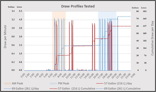
The shape of the draw profiles differ in important ways. The 57 GPD (216 L) profile aligns with common draw profiles with morning weighted draws, consistent with measured hot water energy demand and associated hot water consumption profiles seen in studies stretching back to the 1980s (Masiello and Parker 2002; Fairey and Parker 2004). The 57 GPD (216 L) draw profile was used for tests conducted during warmer weather, with the average daily temperature above 65 °F (18.3 °C). The 69 GPD (261 L) profile has draws more tightly aligned with peak morning and evening hours and was used for tests conducted during cooler weather, with daily average temperatures below 65 °F (18.3 °C). This is appropriate since cooler weather draws will be of larger volume given the lower household inlet water temperature as illustrated in Appendix A. The 57 GPD (216 L) draw profile had draws during the evening load up window, while the larger draw profile did not. The differing shapes of the draw profiles are captured in Figure 1 in the cumulative volume over time for the vertical draw events shown, with the daily volume drawn during load up identified in Table 3.

Table 3. Draw during load-up hours.

Daily draw profile	1-Hour AM load up		1-Hour PM load up		2-Hour AM load up		2-Hour PM load up
	Gallons	Liters	Gallons	Liters	Gallons	Liters	Gallons	Liters
57 Gallon/216 Liters	0	0	3	11	0	0	10	38
69 Gallon/261 Liters	0	0	0	0	0	0	0	0

Control schemes

Up to 11 distinct load shifting schemes implemented during the experimentation were evaluated for each unit. The units were run in their most efficient operating modes (except where different modes are explicitly compared). The general outline for tests was w hours of a morning load up (a period where the stored hot water was temperature was increased as a strategy) followed by x hours of curtailment, then y hours of an afternoon load up followed by z hours of curtailment. Thus, a 1-3-3-4 test protocol indicates a 1-h load up, a 3-h morning curtailment window, a 3-h afternoon load up, and then a 4-h curtailment window during the evening hours. The load up command calls on the water heater to raise the tank temperature up to its set point ahead of the curtailment period. A longer load up period is intended to fully charge hot water storage. This longer duration is important to HPWH compressors with a limited heating capacity compared to larger capacity resistance elements in ERWHs. The curtailment commands used were Shed (S) instructing the unit to avoid operation (within its limits) to allow the present stored energy level of the tank to decrease (whether due to hot water consumption or standby thermal loss), and Critical Peak (CP), instructing the unit to be more aggressive in avoiding operation. Load up commands are issued for the immediate hours ahead of the shed commands.

Experimental results

We examine demand and energy use performance differences among various control schemes for all four production units tested in four ways. First by comparing two curtailment types: Shed versus Critical Peak. Second, we look at 1-h versus 2-h load up period lengths. Third, we look at performance for extended curtailment periods. Finally, we compare two water heater mode settings: hybrid versus efficiency. The prototype unit is evaluated separately. All results are representative of Florida’s warm climate.

Table 4 shows the measured water heater energy (kWh) and power (kW) during the morning and evening peaks to compare the Shed versus the Critical Peak (CP) curtailment commands during both warmer and cooler weather, for all of the production units tested, average for the multiple days tested. The number of test days varied (ranging from 2 to 10), largely depending on available Florida weather such that the cold weather tests comprised the fewest test days. The units are identified as “X: ER 50” for manufacture X, 50 G (189 L) electric resistance, “Y: HP 50” for manufacture Y, 50 G (189 L) heat pump, “X: HP 50” for manufacture X 50 G (189 L) heat pump, and “X: HP 80” for manufacture X 80 G (303 L) heat pump. Daily water heating energy is presented as well.

Table 4. Total daily and peak hours water heater energy and demand: shed versus critical peak.

	X: ER 50			Y: HP 50			X: HP 50			X: HP 80
	Energy	Average peak demand		Energy	Average peak demand		Energy	Average peak demand		Energy	Average peak demand
Schedule	Daily kWh	AM Hours kW	PM Hours kW	Daily kWh	AM Hours kW	PM Hours kW	Daily kWh	AM Hours kW	PM Hours kW	Daily kWh	AM Hours kW	PM Hours kW
57 Gallon/216 liter profile (warm weather)
Baseline	7.43	0.77	0.53	2.35	0.26	0.16	1.86	0.23	0.13	1.76	0.21	0.17
1-3-1-4-S	8.18	0.08	0.07	1.98	0.00	0.00	2.23	0.01	0.04	2.14	0.00	0.00
1-3-1-4-CP	8.04	0.00	0.00	1.85	0.00	0.00	2.11	0.00	0.00	2.04	0.00	0.00
69 Gallon/261 liter profile (cooler weather)
Baseline	11.07	1.64	1.36	2.90	0.28	0.30	3.11	0.31	0.29	2.90	0.16	0.21
1-3-1-4-S	10.96	0.70	0.59	3.31	0.10	0.16	3.35	0.14	0.21	3.39	0.07	0.06
1-3-1-4-CP	10.42	0.21	0.21	2.98	0.14	0.14	3.46	0.03	0.20	3.17	0.00	0.00

Figures 2 and 3 provide the daily average outdoor air and inlet water temperatures for each sample in Table 4 to demonstrate how comparative the temperatures are between baseline and the various events. (Reference Appendix B, Tables B1 and B5 for the daily average outdoor and laboratory air temperature, inlet water temperatures, and minimum delivery temperatures for all schedules listed in Table 4.)

Fig. 2. Outdoor and inlet water temperature, shed versus critical peak, warm weather.

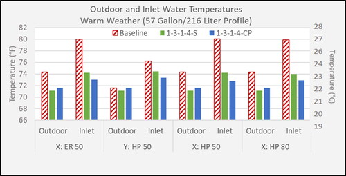
Fig. 3. Outdoor and inlet water temperatures, shed versus critical peak, cooler weather.

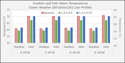
Table 5. Total daily and peak hours water heater energy and demand: 1-h versus 2-h load up.

	X: ER 50			Y: HP 50			X: HP 50			X: HP 80
	Energy	Average peak demand		Energy	Average peak demand		Energy	Average peak demand		Energy	Average peak demand
Schedule	Daily kWh	AM hours kW	PM hours kW	Daily kWh	AM hours kW	PM hours kW	Daily kWh	AM hours kW	PM hours kW	Daily kWh	AM hours kW	PM hours kW
69 Gallon/261 Liter Profile (Cooler Weather)
Baseline	11.07	1.64	1.36	2.90	0.28	0.30	3.11	0.31	0.29	2.90	0.16	0.21
1-3-1-4-S	10.96	0.70	0.59	3.31	0.10	0.16	3.35	0.14	0.21	3.39	0.07	0.06
2-3-2-4-S	9.58	0.33	0.24	2.47	0.08	0.09	2.84	0.07	0.10	n/a	n/a	n/a
1-3-1-4-CP	10.42	0.21	0.21	2.98	0.14	0.14	3.46	0.03	0.20	3.17	0.00	0.00
2-3-2-4-CP	9.38	0.20	0.18	2.40	0.08	0.09	2.85	0.00	0.10	2.79	0.00	0.00

During the warmer weather and the 1-3-1-4 scheme, all units demonstrated complete or near complete curtailment for both morning and evening peak demand windows. However, the Critical Peak load reduction was more effective than the Shed command. The “Y: HP 50” unit had reduced daily energy use over baseline during the 57 G (189 L) curtailment schedules shown. This was not unusual for this unit, for which we observed as much as a 7 °F (∼4 °C) drop in outlet temperature during curtailment draws coincident with lower total energy use.

For the electric resistance unit, average morning demand during warmer weather was reduced by 0.69 kW with Shed, and 0.77 kW (100%) with CP instructions. Average evening demand was lower by 0.46 kW with Shed and 0.53 kW (100%) with CP. There was an 8-10% daily energy penalty where consumption increased with the curtailment under both the Shed (0.75 kWh/day) and the CP (0.61 kWh/day) during warmer weather tests. In this case, the baseline consisted of warmer days as would be experienced in Central Florida summers with warmer inlet water temperatures. Increased energy use was associated with load up and recovery that did not occur at those times during baseline.

With the 1-3-1-4 scheme during cooler weather, all of the units struggled to make it through the curtailment period without using electric resistance heating at some point during this test. During the Shed tests, average demand was reduced by 0.08 − 0.18 kW among all HPWHs. During the CP tests, average demand reduction for “Y: HP 50” was similar to that of the Shed tests. In contrast, both morning and evening reductions were greater under CP tests than under Shed tests, for both “X: HP 50” (0.28 kW AM, 0.09 kW PM) and “Y: HP 80” (0.16 kW AM, 0.21 kW PM) – which was complete curtailment for the larger volume tank. These results seem to indicate that during cooler weather, the CP command was superior for load reduction, especially with the larger volume tank. The daily average energy used during CP tests was increased over baseline for all HPWHs: 0.08 kWh, 0.35 kWh, and 0.27 kWh for the “Y: HP 50”, “X: HP 50”, and the “Y: HP 80”, respectively. Daily energy use was also up for the Shed testing, though ambient and inlet water temperatures were slightly cooler thus slightly more favorable.

For the electric resistance unit, average morning demand during cooler weather was reduced by 0.94 kW during Shed, and 1.43 kW with CP instructions. Average evening peak demand was down by 0.77 kW with Shed and 1.15 kW during CP tests. Daily average energy use was slightly reduced over baseline during both the Shed (0.11 kWh/day) and the CP (0.65 kWh/day) tests. It must be understood, however, that baseline demand and energy use is much higher for an ERWH, so results would be very different when comparing the controlled HPWH to the ERWH – an important point as ERWHs are substituted with grid-connected HPWH. This is also emphasized since ERWH are by far the most prevalent type of electric water heating system that will be substituted against.

Results are displayed graphically in Figures 4 and 5, showing daily water heating draw and water heater electric demand plots for the 1-h Shed and Critical Peak control schemes to illustrate some of the cooler weather results summarized in Table 4. The plots are a composite of several days during the same command structure and present the electric demand daily load profile of a 50 G (189 L) HPWH during a command structure comprised of a 1-h morning load up, a 3-h curtailment, a 1-h afternoon load up, and a 4-h curtailment (i.e., 1-3-1-4), comparing the Shed to the CP command. Figure 4 includes the backdrop of the manufacturer X’s electric resistance 50 G (189 L) tank, with its demand indicated in by the sold red line. The shaded areas represent the hours of load up and curtailment, for morning (peach) and evening (blue). Figure 5 provides the same results on a magnified scale without the ERWH.

Fig. 4. 1-3-1-4-S compared to 1-3-1-4-CP command structure, with ERWH baseline.

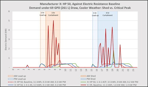
Fig. 5. “X: HP 50” unit under 1-3-1-4-S compared to 1-3-1-4-CP structure.

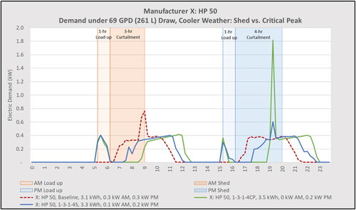
The dashed red line is the baseline condition, the blue is the Shed curtailment, and the green is the CP curtailment. Both command schemes take equal advantage of the 1-h load up. During the morning peak window, actions from the Shed command were not strong enough to keep the unit from engaging during the curtailment window, however the CP command does a near perfect job of eliminating demand. Curtailment performance was similar in the afternoon, however the curtailment window was an hour longer and under the CP test, electric resistance was triggered before the window ended.

This difference is reflected in Table 4, with average peak morning demand of 0.14 kW for the Shed tests versus 0.03 kW for the CP tests. During the afternoon, the Shed scheme again fails to make it through the curtailment window. And while the CP scheme pushes demand off a while longer, the water heater reaches its threshold and responds with a small level of resistance heating to recover. The net result was that both the Shed and the CP scheme had similar average demand during the afternoon curtailment window; 0.21 kW and 0.20, for Shed and CP, respectively.

Another variation among the tested schemes included the length of the load up period. Table 5 shows the average measured water heater kW during the morning and evening peaks to compare 1- to 2-h load ups, and for both Shed and CP curtailments. (Reference temperature data in Appendix B, Tables B2 and B6.) For this comparison, we examine how the units performed during colder weather testing which generated more curtailment challenges.

Table 6. Baseline performance for X:HP80 hybrid versus efficiency mode, under 57 G (216 L) per day draw profile.

	X: ER 50							X: HP 80
Baseline	Temperature				Energy	Average peak demand		Temperature				Energy	Average peak demand
Mode	Daily average outdoor °F/°C		Daily average inlet °F/°C		Daily kWh	AM hours kW	PM hours kW	Daily average outdoor °F/°C		Daily average inlet °F/°C		Daily kWh	AM hours kW	PM hours kW
Hybrid	76.7	24.8	84.4	29.1	6.6	0.70	0.47	76.7	24.8	84.5	29.2	1.9	0.22	0.15
Efficiency	79.9	26.6	85.9	29.9	6.2	0.62	0.47	79.9	26.6	85.8	29.9	1.5	0.17	0.16

Under cooler conditions, both of the 50 G (189 L) HPWHs demonstrated improved curtailment using a 2-h load up scheme relative to a 1-h, for both Shed and CP tests. Average peak demand during the 2-h load up for both the Shed and CP testing was down by 0.20–0.31 kW (AM) and 0.19–0.21 kW (PM), depending on manufacturer. Demand for the larger capacity 80 G (303 L) HPWH was already completely eliminated under the 1-h CP testing, so the 2-h load up was not necessary.

These same trends were demonstrated with the electric resistance water heater, but with greater amplitude given its higher baseline demand. The 2-h Shed tests resulted in average peak demand reductions of 1.31 (AM) and 1.12 kW (PM) with daily energy use reduced by 1.49 kWh, and the 2-h CP tests performed slightly better with average peak demand reductions of 1.44 (AM) and 1.18 kW (PM) with daily energy use reduced by 1.69 kWh. Three hour load up periods were also tested, but showed no additional peak demand reduction. If an uncontrolled ERWH is considered the winter baseline, the 1-3-1-4-S with a controlled HPWH of same volume reduced AM water heater peak demand by 1.50 − 1.61 kW or from 91 to 98%. This comparison is important since ERWH are by far the common water system heating type in the Southeastern U.S.

A third variation among the tested schemes was the length of the curtailment period, in which the average measured water heater kW during the morning and evening peaks were evaluated to compare 5-h morning and 6-h evening curtailments during the more aggressive CP instruction, during both warmer and cooler weather.

Under warmer ambient conditions, all of the HPWHs tested demonstrated nearly complete demand reduction for the entire 5-h and 6-h curtailment periods tested given 2-h morning and afternoon load ups. Average curtailment ranged from 0.08 kW to 0.18 kW among all three HPWHs. Daily average energy use was largely unchanged, however somewhat reduced during the CP testing over baseline conditions. The ERWH also performed well, though the morning curtailment was incomplete, with a reduction to 0.21 kW from the 0.76 kW baseline, or 0.55 kW, which suggests that differences in load control strategies are not so important during summer. The potential load reduction is much lower during warmer weather (80–180 Watts).

Demand reductions were present across all units during cooler weather testing, but none of the units were able to completely eliminate peak demand. Still, with greater demand during these cooler days, and just slightly less favorable conditions during CP testing (with inlet water temperatures about 2 °F (∼1 °C) warmer), reductions are impressive. Under the 2-5-2-6-CP cooler weather tests, there was little difference from one manufacturer to the other for the 50 G (189 L) size. The HPWH reduced morning (AM) demand by 0.11 to 0.12 kW and afternoon (PM) demand 0.02 to 0.07 kW. The larger 80 G (303 L) unit was similar in reducing morning demand (0.13 kW), but superior in offsetting evening demand with a 0.12 kW reduction. Daily average energy use decreased slightly for the “Y: HP 50” unit, but increased by 0.35 and 0.38 kWh, for “X: HP 50” and X: HP80, respectively.

Under the 2-5-2-6-CP scheme, the overall demand reductions for the ERWH were greater in cooler weather than they were for the warmer baseline/test comparison. Under the 2-5-2-6-CP cooler weather tests, average peak demand was reduced by 0.57 kW (AM) and 0.56 kW (PM) and daily average energy use was essentially unchanged from baseline. For comparison, under this same test the HPWH showed average peak demand reductions of 0.78 − 0.87 kW (AM) and 0.79 − 0.89 (PM), depending on manufacturer and tank volume.

For the ERWH, the baseline morning peak demand of 0.76 and daily average 7.43 kWh for the more typical Florida weather used in the warm weather baseline is on par with findings for a 153-sample study of non-gas Florida homes, which found average water heating morning demand of 0.71 kW and an average annual hot water energy consumption of 6.37 kWh/day (Masiello and Parker 2002). Note that this is the diversified demand over 150 water heaters whereas our laboratory test data is from a single unit. Thus, in a population of water heaters, the demand we saw in the laboratory tests would almost certainly be lower although trends would be similar.

One concern within water heater load control programs is that users may have insufficient hot water during large draw events or during lengthy control periods. Within the experiment, thermocouples at the tank outlet measured outlet water temperature during draw events. Under the favorable Florida test conditions we saw no evidence of the problem of low temperature hot water draws either with the 57 GPD (216 L) or 69 GPD (261 L) draw profiles, even during cooler conditions– an important consideration for using the CTA-2045 standard instead of traditional direct load control. Outlet temperatures rarely fell below 115 °F (46.1 °C), with a low of 112.9 °F (44.9 °C). The 80 G (303 L) unit’s lowest measured outlet temperature for these tests was 119.1 °F (48.4 °C). More details on wintertime hot water delivery temperatures are available in Appendix B.

Efficiency versus hybrid mode

We conducted experiments to examine demand and energy use performance differences between the HPWH’s most energy efficient mode, herein called “efficiency”, and the unit default mode, or “hybrid”, water heater setting which typically uses more resistance heating to make sure the hot water supply is not exhausted (different terminologies are used among manufacturers for similar modes). Data for this evaluation were collected during warmer weather and the 57 GPD (216 L) draw profile. Again, test results are relevant to units in warm garage environments.

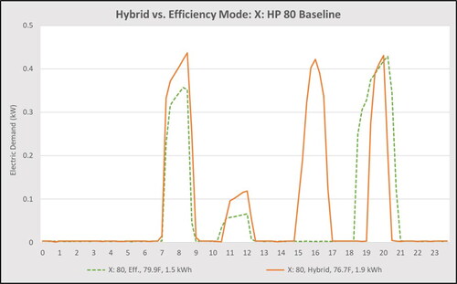
We first assessed performance differences under baseline conditions when units were not controlled. A baseline comparison was conducted on the “Y: HP 80.” Daily energy use, peak demand results and daily average outdoor air and outlet water temperatures are provided in Table 6.

The ERWH data (i.e., X: ER 50) are presented to demonstrate the operational similarity between the hybrid mode and the efficiency mode test periods. The “Y: HP 80” exhibited lower energy use when operating in the efficiency mode, during which time weather was only slightly more favorable (warmer) than during the hybrid mode. The daily demand profiles for both modes are plotted in Figure 6. The power draw during hybrid mode at 15:00 h is notably different to the operation during the efficiency mode, revealing a portion of the the additional 0.38 kWh which altered the demand profile during afternoon hours. Daily energy use in the efficiency mode is 20% less than in hybrid mode and the AM peak demand was about 25% lower.

Fig. 6. Baseline demand profile for “X: HP 80” hybrid versus efficiency mode, under 57 G (216 L) per day draw profile.

The 2-3-2-4-S test was conducted on all units in both modes with comparable days – both in terms of the daily average outdoor temperature and the inlet water draw temperature. Energy and demand results are summarized in Table 7. (Reference temperature data in Appendix B, Tables B3 and B7.) In this table, the ERWH performance is also provided to demonstrate the operational similarity between the hybrid mode and the efficiency mode test periods.

Table 7. Performance during 2-3-2-4-S command scheme, hybrid versus efficiency mode, under 57 GPD (216 L) draw profile.

	X: ER 50			Y: HP 50			X: HP 50			X: HP 80
2-3-2-4-S	Energy	Average peak demand		Energy	Average peak demand		Energy	Average peak demand		Energy	Average peak demand
Mode	Daily kWh	AM hours kW	PM hours kW	Daily kWh	AM hours kW	PM hours kW	Daily kWh	AM hours kW	PM hours kW	Daily kWh	AM hours kW	PM hours kW
Hybrid	7.6	0.16	0.00	1.8	0.04	0.00	2.3	0.05	0.00	2.3	0.05	0.00
Efficiency	7.6	0.00	0.00	1.8	0.00	0.00	2.0	0.06	0.03	1.9	0.06	0.00

Manufacture Y’s 50 G (189 L) HPWH performed nearly identically under the hybrid and efficiency modes, both in terms of energy use and peak demand. Both of manufacture X’s HPWHs showed reduced energy use in the efficiency mode over hybrid, however unit mode hardly impacted demand during the peak window curtailment.

Summarized in Table 8 are the energy and demand results from a more aggressive communications scheme, 1-5-1-6-CP, which was tested on the “Y: HP 50” and the “X: HP 80.” (Reference temperature data in Appendix B, Tables B4 and B8.) Daily energy use was nearly the same between modes for each unit. Morning curtailment was complete in all cases. As highlighted in Figure 7, the afternoon curtailment was slightly improved for both units during the efficiency mode, although the differences were small and the statistical significance is unknown.

Fig. 7. 1-5-1-6-CP demand profile for “Y: HP 50” and “X: HP 80” hybrid versus efficiency mode, under 57 G (216 L) per day draw profile.

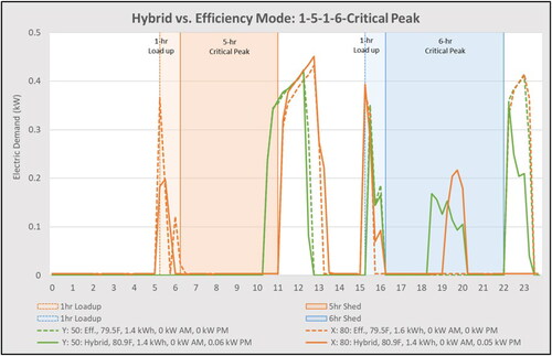
Table 8. Performance during 1-5-1-6-CP command scheme, hybrid versus efficiency mode, under 57 G (216 L) per day draw profile.

	X: ER 50			Y: HP 50			X: HP 80
1-5-1-6-CP	Energy	Average peak demand		Energy	Average peak demand		Energy	Average peak demand
Mode	Daily kWh	AM hours kW	PM hours kW	Daily kWh	AM hours kW	PM hours kW	Daily kWh	AM hours kW	PM hours kW
Hybrid	6.0	0.00	0.00	1.4	0.00	0.06	1.4	0.00	0.05
Efficiency	6.8	0.00	0.00	1.4	0.00	0.00	1.6	0.00	0.00

In summary, tests conducted in a hot humid climate, with the HPWH in efficiency mode demonstrated some ability to reduce energy use over the hybrid mode, both during baseline and during the CTA-2045 curtailment scheme where conditions were tightly matched between tests. Both modes demonstrated the ability to nearly perfectly curtail demand during the peak window under the 2-3-2-4-S scheme with mild conditions. Under a more aggressive 1-5-1-6-CP test, afternoon curtailment is slightly improved if the unit is in efficiency mode. One conclusion is that while efficiency mode appeared to reduce HPWH daily energy by as much as 20% over hybrid mode for a tested manufacture, the impact peak load reduction for Shed or Critical Peak commands did not differ appreciably.

Experimental results of CTA-2045-B prototype

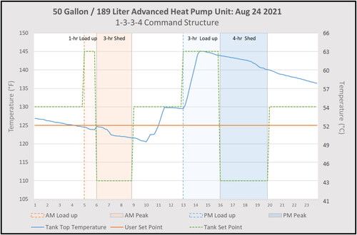
For the prototype 50 G (189 L) HPWH with the advanced load up capabilities of CTA-2045-B, we sent an advanced load up command which allowed the water to be heated above the tank set point (15 °F (8.3 °C), in our experiments). Such units use an integrated mixing valve to moderate the delivery temperature to prevent scalding users. For the experiments, we allowed the tank set point to approach 145 °F (62.8 °C). (With manufacturer guidance, researchers determined that the tank set point needed to be 5 °F (2.8 C) above the desired user set point to prevent the mixing valve from requiring recalibration. For example, a 130 °F (54.4 °C) tank set point was needed to deliver water at 125 °F (51.7 °C).) Figure 8 demonstrates how the tank temperature of the heat pump with advanced load up varied during a typical summer day under load control. Note that during the 3-h afternoon advanced load up, the temperature taken at the top of the tank (blue) rises from 130 °F (54.4 °C) to 145 °F (62.8 °C) in about 45 min under the summer operating conditions in a hot humid climate.

Fig. 8. Temperatures for manufacturer Z 50 G (189 L) HPWH with CTA-2045-B protocol capability including advanced load up capability.

The prototype unit was tested with the 1-3-1-4-S, 1-3-3-4-S, and the 2-5-2-6-S control schemes under the winter and 69 GPD (261 L) draw profile. Curtailment was complete, or nearly so, under all tests; outperforming the similarly sized units without the advanced load up capability. This translated into average demand reduction of 0.48 kW and 0.40 kW, for the morning and evening peak periods, respectively. The 1-3-3-4-S test, presented in Figure 9, also shows a sizeable energy reduction (1.01 kWh per day, or 23%). For comparison, performance results of all three tests and those of baseline conditions are presented in Table 9.

Fig. 9. Manufacture Z prototype CTA-2045-B unit under 1-3-3-4-S structure.

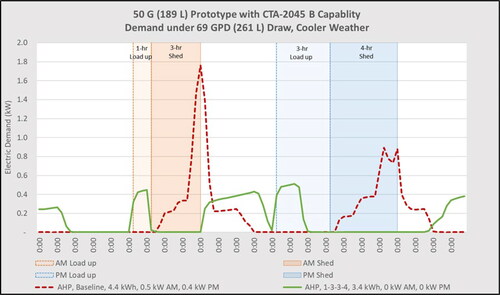
Table 9. Total daily and peak hours water heater energy and demand of advanced load up prototype.

CTA 2045-B Unit	Temperature				Energy	Average peak demand
	Daily average outdoor °F/°C		Daily average inlet °F/°C		Daily kWh	AM hours kW	PM hours kW
69 Gallon/261 Liter Profile (Cooler Weather)
Baseline	60.6	15.9	71.8	22.1	4.4	0.48	0.40
1-3-1-4	58.5	14.7	66.5	19.2	5.0	0.00	0.00
1-3-3-4	60.4	15.8	72.4	22.4	3.4	0.01	0.00
2-5-2-6	58.6	14.8	68.2	20.1	4.5	0.01	0.01

Experimental reproducibility

One concern with the testing was repeatability of the experiments across the different draw patterns. In fact, draw profile and electric demand profiles were remarkably consistent, showing reliable reproducibility. Although these tests were successfully done for all of the tested water heaters, in Figure 10, we show repeated tests for the prototype unit with the 0-5-4-6-S load control profile evaluated on 13 different days. This demonstrates practical experimental repeatability giving confidence in measured results and differences. Repeatability was strongest when outdoor conditions were very similar among test days, as in this example where the daily average outdoor temperature ranged from about 75 °F (24 °C) to 83 °F (29 °C). Greater variability in energy profile was exhibited however, when the outdoor conditions varied more greatly between test days which was more typical of the cooler weather testing. Measuring field impacts will require large samples for many of the small influences that were observed with deterministic draws in a laboratory. This occurs because of the probabilistic nature of hot water draws and varying conditions across a population of water heaters. This is clearly seen in earlier one-minute data in a previous project monitoring 50 electric water heaters. Calculating necessary sample size can be based on specific levels of precision and accuracy (Fenaughty, Parker, and Martin 2017).

Fig. 10. Repeated testing of the 0-5-4-6-S profile on 13 days of similar weather.

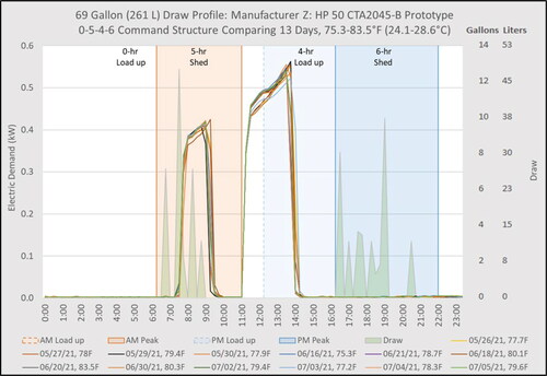
The thirteen repeated tests in Figure 10 for 0-5-4-6-S for the unit show an average morning peak demand of 0.19 (+0.03) kW giving a good indication of the experimental variation in the laboratory testing.

Caveats

This laboratory evaluation of the potential impacts of load-controlled HPWHs has important limitations. The testing was done in Central Florida, where the daily average outdoor temperature for the tests evaluated varied between 48 °F and 80 °F (9.1 °C − 26.8 °C), favorable operating conditions for heat pumps. This also means that inlet water temperatures were high (daily average inlet draw temperatures for the conducted tests ranged varied between 64 °F and 86 °F (17.8 °C − 30.1 °C), making it easier to interrupt the water heaters without activating the heat pump compressor or back up electric resistance heating. Many other locations experience much colder temperatures, both outdoors, in basements, and for the inlet water temperatures than does Central Florida. Still these test results are likely relevant to the U.S. southeast and to other mild locations along the U.S. southern latitudes.

Another caveat is that the tests were conducted in garage-like conditions thus results are applicable to garage-located water heaters and less applicable to units installed in an interior closet, for example, which is also commonplace in Florida.

A final limitation is that the draws examined in the tests are necessarily deterministic for experimental repeatability. In actuality, household hot water draws are probabilistic and vary stochastically over time in a complex way depending on the distribution of hot water draw event variations across households (e.g. Ritchie, Engelbrecht, and Booysen 2021). Thus, results here are indicative, rather than predictive. In particular, diversified demand over a large population of water heaters will likely show peak demand values in the field are lower—typically by about 50% – than the laboratory values seen for the specific draw profile (Masiello and Parker 2002).

Conclusions

We completed a detailed laboratory evaluation of grid-connected heat pump water heaters (HPWH), using advanced communication protocols to demonstrate performance in comparison to conventional electric resistance water heaters (ERWH). The investigation applied different CTA-2045 curtailment control designs under two different water draw profiles representing average summer and average winter hot water consumption. The evaluation was intended to represent single-family homes located in Central Florida. Detailed temperature, energy, peak window power demand, and flow data were obtained.

We evaluated two fundamental strategies for cutting peak demand under both warm and cooler conditions; one with a 1-h “load up” where the water heaters are activated before the utility peak demand period and also a 2-h load up. The impact of both the Shed and Critical Peak commands were assessed. The HPWH units were also evaluated for differences operating under hybrid versus efficiency modes. Equipment from two major water heater manufacturers was evaluated using equipment from two major water heater manufactures using the CTA-2045 controls with units set in their most efficient operating mode. Two storage volumes, 50 G/189 L and 80 G/303 L, were evaluated for one manufacturer. We compared baseline (no load control) for both ERWH and HPWH to assess the potentials of load control with grid-connected HPWH. And finally, we investigated the potential benefits of the CTA-2045-B protocol, applying tests to one prototype unit with the advanced load up capability. Problems were encountered with the prototype unit, but the authors remain convinced of the value of advanced load up using the 2045-B protocol. Further research is indicated.

Warmer-summer conditions

• Baseline peak demand was only about 0.77 kW for the ERWH during the morning period and 0.53 kW during the evening peak. These were undiversified values from a single tested system.

• For the HPWHs, the baseline peak was only about 0.21–0.26 kW (morning) and 0.13–0.17 kW (evening). Thus, grid-connection summer load shed potentials appear much lower given the HPWH baseline.

• Load control strategies in summer are nearly equally effective. Short 1-h load ups work for reducing water heat demand both for morning and evening control windows. Grid connected HPWH were able to largely eliminate demand during both peak windows which was not true for the grid connected ERWH.

• The Shed command is as effective as the Critical Peak (CP) command for reducing demand. Daily water heating energy use is very slightly elevated by control (typically <5%) for Manufacturer X, while it was slightly reduced for Manufacturer Y.

• The 80 G (303 L) storage tank offered no apparent performance advantage over the 50 G (189 L) in summer.

• Load control for the ERWH increased daily water heating energy by 8–10%. The Shed command was not as effective as the CP command for reducing morning and evening demand.

Cooler conditions

• Baseline peak demand was 1.64 kW for electric resistance during the morning, and 1.36 kW during the evening peak periods. These are undiversified values from a single water heater.

• For the HPWH, the baseline peak was only 0.16 kW –0.31 kW (morning) and 0.21 kW–0.30 kW (evening). The lower values showed the importance of the 80 G (303 L) tank in reducing peak demand, even without load control.

• Load control strategies showed real differences. Short 1-hour load ups (1-3–1-4 strategy) do not work as well. However, grid connected HPWH were able to nearly eliminate the morning water heating peak if the CP control command was used for Manufacturer X.

• Grid-connected ERWH was only able to cut morning peak demand by about 57% with the Shed command given a 1-hour load up.

• A 2-h load up strategy (e.g. 2-3-2-4) looks important to obtain good demand reduction in winter with the Shed command and the 50 G (189 L) tank; much less so with the 80 G (303 L) tank. There is no significant energy increase with a 2-h load up observed.

• The ERWH was not entirely able to eliminate the morning or evening peak demand with a 2-h load up; the HPWH water heaters often had complete or near complete peak demand reduction.

• Measured outlet water delivery temperatures in testing revealed no incidences where the household was found to run out of hot water, with the lowest temperature measurement of 112.9 °F/44.9 °C.

A fundamental conclusion is that load control strategies for grid connected HPWH for mild to warm weather are effective, but do not matter as much as the magnitude of water heating energy, and demand is low (0.08 kW to 0.18 kW) for the uncontrolled baseline. Grid connected HPWH have most potential during cooler weather, when peak demand is great. The greatest reductions were seen using the CP command. The ERWHs had winter morning peak demand up to 1.6 kW, however diversified demand in a large population of water heaters is likely about half this value. (Masiello and Parker 2002).

In our testing, HPWHs tended to use more resistance electricity - and hence greater energy - when they were in the “hybrid” mode than when they were in “efficiency” mode. Units are shipped from the manufacturer in hybrid mode. As expected, the owner-selected efficiency modes showed as much as 20% lower water heating energy. While there are differences among manufacturers, reduced demand from the load curtailment commands generally appeared to be similar in both the hybrid and efficiency modes, although this may not be true under colder test conditions.

Our investigation of the CTA-2045-B protocol showed promising results even though the prototype system encountered problems. The prototype unit tested demonstrated complete or nearly complete peak demand reduction in all cases, outperforming similarly sized units that did not have the advanced load up capably.

We found inlet water temperatures to vary significantly over time, even within the same location, and also seasonally so that volumetric hot water draws are much greater in winter to provide suitable bathing/shower delivery temperatures. We propose a new simple method to estimate water heater inlet temperatures based on ground temperatures at the frost line where inlet water pipes are buried. We found that large levels of in-ground heat transfer to street-level water lines are so pronounced that they significantly reduce the observed difference in source water temperatures, such as those from reservoir, surface, or well. We also suggest that such a method is critical for evaluating HPWHs since seasonal variations in ground inlet water temperature and impacts on energy load both from increased delta T and increased volumetric load will place the greatest load on HPWHs at the time when their COP and capacity are lowest. (As presented in Appendix A.) The altered seasonal volume is important to use for load control experiments with HPWH where capacity may be lower with winter air temperatures. The resulting reduced capacity may activate back-up resistance heating that can mar potential efficiency gains.

Disclosure statement

No potential conflict of interest was reported by the author(s).

Additional information

Funding

This work was supported by the US Department of Energy (DE-AC05-76RL01830).

Appendix A

Calculating household inlet water temperatures

The hot water system inlet water temperature is a fundamental parameter to estimate the water heating energy loads in residential systems. Given that systems commonly raise hot water temperatures to approximately 125 °F (51.7 °C), the energy to reach that water temperature is strongly governed by the difference of the target temperature to the mains water entering the hot water storage tank or system. As observed and documented by Burch and Christiansen (2007), the inlet water temperature varies significantly around the U.S., but also with a large seasonal variation in each location.

Until recently, the seasonal influence is often not considered, but potentially has a large impact. This influence occurs not only due to the energy required to heat a given quantity of water but also because the cooler temperatures in winter increase the mix of hot water for hot water end uses such as bathing and washing that are sensitive to skin temperature (Parker, Fairey, and Lutz 2015). This influence has special significance for air source heat pump water heaters, which perform less efficiently in winter months when shortfall in capacity is made up by use of electric resistance heat. This means that not only are air temperatures lower in winter for the air-source compressor, but also that based on the lower inlet water temperature, water heating loads are larger as well.

One advantage of the laboratory test in Central Florida is that not only did we have the measured inlet water temperature during hot water draws, but we also had the ground temperatures measured on site from 1 to 15 feet, in one foot increments. We noticed that the ground temperature on site seemed to closely track the daily inlet water temperature. Indeed other researchers in Poland and the Netherlands have observed the same phenomenon, although with some variation given the water source; they indicated that the ground temperature at a 1 m depth will best characterize delivered inlet water temperatures (Moerman et al. 2014).

We propose, based our these observations, that estimating the ground temperature at the depth which the inlet water piping in a location can be accomplished by estimating the ground temperature at the depth the water lines are buried.

We propose a simple generalized method that considers the geographical location and the buried depth of the pipe, and the soil properties to estimate the water heating inlet water temperature. While specific soil properties are uncertain for a given site, typical values can often be used, modified by pipe depth. This is appropriate since water lines tend to be buried 1–2 feet (0.3–0.6m) below the frost depth at geographic locations. The depth of the appropriate frost line around the U.S. can be seen in Figure A1.

That undisturbed ground temperature relationship estimates the temperature of soil at depth (Equation A1) has proved accurate against field observation (Kusuda and Achenbach 1965). The deep well water temperature in various locations around the U.S. was measured by the U.S.G.S. (Collins 1925). Maps of the well temperatures as well as surface temperature amplitude are given in Labs et al. (1988).

Equation A1. Calculation of undisturbed ground temperature for estimating inlet water temperature $$T=\mathrm{ }{T}_{\mathit{mean}}\mathrm{ }\text{-}\mathrm{ }{T}_{\mathit{amp}}\mathrm{ }\mathrm{*}\exp \hspace{0.17em}\left(-Z\text{ * }\sqrt{\frac{\pi }{365\mathrm{*}\alpha }}\right)$$ $${\mathrm{*}}_{\cos }\left(\frac{2\pi }{365}\mathrm{*}\left[1_{\mathit{year}}-1_{\mathit{shift}}\text{-}\mathrm{ }\frac{Z}{2}\mathrm{ }\mathrm{*}\sqrt{\frac{365}{\pi \mathrm{*}\alpha }}\right]\right)$$ where: T = temperature of soil; T_mean = mean surface temperature (average air temperature). The temperature of the ground at an infinite depth will be this temperature. T_amp = amplitude of surface temperature (the maximum surface temperature will be T_mean + T_amp and the minimum value will be T_mean * T_amp); Z = depth below the surface; Α = thermal diffusivity of the ground (soil); 1_year = current time (day); 1_shift = day of the year of the minimum surface temperature.

The governing soil properties are difficult to determine, but there are references such as in Table A1. It is suggested the dry vs. damp be the main properties exercised depending on location for determining inlet water temperature. Soil thermal diffusivity is the primary property of interest for the calculation method, although one observes from the data that this property varies by a factor three.

Predicted versus measured temperature

We found that the proposed method for estimating water inlet temperatures matched the measured temperatures in Cocoa, Florida in a convincing way. The following parameters in Table A2 were used in the evaluation of the calculation method.

Air temperature data were taken from a Cocoa, Florida test facility. The amplitude, light damp soil property data were taken from Labs et al. (1988), presented in Figure A2.

It is seen that the monthly prediction of the inlet water temperature is quite accurate. The prediction is nearly perfect for daily average inlet temperatures against the ground temperature at a 2 foot depth. Whereas lab temperature is significant for hourly draws, it is not for daily draws. This means that lab temperature (or garage) influences inlet water temperature slightly depending on time of day, but not in a fashion that will likely impact water heating energy use. Ground temperature is the overriding influence. The regression and statistical parameters are given in Figure A3.

As suggested by the above regression, the predicted time series for each hour appears equally good. The relevant comparison of measured inlet water temperature and the prediction along with air temperatures are shown in Figure A4 to allow a visible indication of the success of the method in predicting inlet water temperatures.

The importance of knowing the appropriate inlet water temperature for seasonally representative tests is illustrated for the analysis done to support the laboratory testing. This is based on the analytical method suggested by Parker, Fairey, and Lutz (2015). Here hot water gallons per day is based on empirical and physical relationships in that paper, as presented in Equation A2.

Equation A2. Calculation of gallons of water per day per home. $$\mathrm{HWgpd}\mathrm{ }=\mathrm{ }22\text{ * }\left(\text{Occupants * }{\text{F}}_{\text{mix}}\right)\mathrm{ }+\text{ CWgpd }+\mathrm{ }\mathrm{DWgpd}$$ where: F_mix = the mix of hot-to-cold water to reach desired water temperature for bathing, faucets $${\text{F}}_{\text{mix}}=\mathrm{ }\left[1\right[({\text{T}}_{\text{set}}\mathrm{ }–\mathrm{ }{\text{T}}_{\text{mix}})/\left(\right({\text{T}}_{\text{set}}\mathrm{ }–\mathrm{ }{\text{T}}_{\text{inlet}}\left)\right]$$ T_set = 125 °F; T_mix= desired hot water temperature for skin sensitive end uses (105 °F); CWgpd = clothes washer gallons per day; DWgpd = dishwasher gallons per day.

For a family of 4 persons in Central Florida we can estimate from Figures A3 and A4 that the June–September inlet water temperature is 83.5 °F and 71.0 °F for December – February. This means that F_mix is 0.52 for summer (52% hot water needed for showers, bathing etc.) versus 0.63 in winter. With the draw from a clothes washer and dishwasher approximated at 8.6 gallons per day for 4 persons, the indicated daily hot water needs in summer are about 54.4 G (206 L) versus 64.0 G (242 L) in the winter months. This is just under a 20% difference in the hot water volume from winter to summer in the Central Florida location.

The illustrated differences indicate the importance of accounting for seasonal variation inlet water temperature, not only for raising the inlet water to the set temperature, but also for the volume of hot water to be heated. This modeled difference approximately mirrors the delta of our two draw conditions with 57 G (216 L) and 69 G (261 L) used for the laboratory testing in our experiments, for summer and winter, respectively. Accounting for these two effects are particularly important in comparative testing for HPWH systems since they tend to be less efficient in winter with lower air temperatures for the compressor and also more likely to encounter backup resistance heating from reduced thermal capacity against the higher volumetric water heating loads during winter months. This difference is even more critical in load shedding experiments where hot water capacity may be pushed to its upper acceptability limit for bathing and showers.

Fig. A1. Frost line depth in inches around the U.S. (Source: U.S. Weather Bureau).

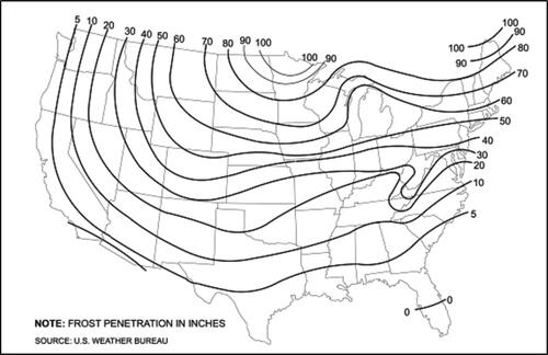
Fig. A2. Predicted vs. measured inlet water temperature in Cocoa, FL, 2021.

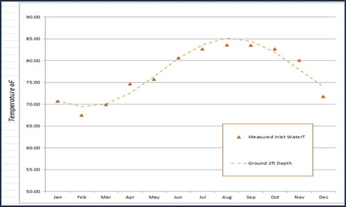
Fig. A3. Regression of measured inlet water temperature against prediction with hourly data.

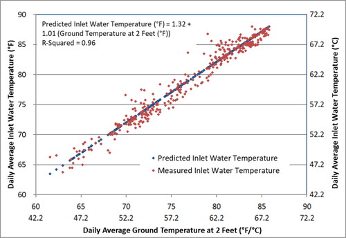
Fig. A4. Comparison of measured (blue) inlet temperature, ground temperature and outdoor air temperature.

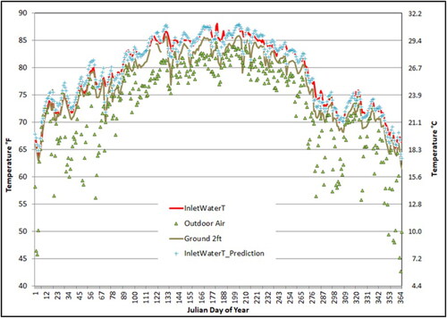
Table A1. Typical soil physical properties.

Soil type	Density	Specific heat	Conductivity	Diffusivity
	lb./ft.^3	Btu/lb.-F	Btu/hr./lb.-F	Ft.^2/day
Heavy soil, wet	117	0.30	1.40	0.96
Heavy soil, damp	131	0.23	0.75	0.60
Heavy soil, dry	125	0.20	0.50	0.48
Light soil, damp	100	0.25	0.50	0.48
Light soil, dry	90	0.20	0.20	0.27

Table A2. Method estimate versus prediction for inlet water temperature of 2021 data.

Variable		Value	Unit
Conductivity		0.50	k: Btu-hr/ft-°F
Soil density		100	lbs/ft3
Soil specific heat		0.25	Btu/lb-F
Soil diffusivity		0.48	ft^2/day
Pi		3.14	Dimensionless
Depth		2	Ft
Average air temperature		75.2	°F – Orlando, FL
Average surface temperature amplitude		9	°F – Orlando, FL
Phase constant		35	Days
Average groundwater temperature at 2 feet		77.3	ft^2/day – Orlando, Fl
Month	Julian day	FRTF data: 2 feet depth
Jan	15	70.82
Feb	46	69.41
Mar	74	70.02
Apr	105	72.61
May	135	76.37
Jun	166	80.50
Jul	196	83.66
Aug	227	85.17
Sep	258	84.50
Oct	288	81.93
Nov	319	78.02
Dec	349	74.04
Average		77.25

Appendix B.

Daily average outdoor, lab, and inlet, and minimum delivery temperatures

 

Table B1. Shed versus critical peak: daily average outdoor, lab, and inlet, and minimum delivery temperatures (Fahrenheit).

	Sample size (days)	X: ER 50				Y: HP 50
		Outdoor	Lab	Inlet	Delivery	Outdoor	Lab	Inlet	Delivery
57 Gallon/216 liter profile (warm weather)
Baseline	7(4)	74.3	79.5	80.0	122.4	71.5	77.0	76.2	125.3
1-3-1-4-S	8	71.1	75.8	74.2	122.4	71.1	75.8	74.4	118.2
1-3-1-4-CP	4	71.6	79.0	73.0	122.3	71.6	79.0	73.3	121.5
69 Gallon/261 liter profile (cooler weather)
Baseline	10	60.8	64.2	70.2	123.7	60.8	64.2	70.2	118.8
1-3-1-4-S	5	59.5	62.0	67.2	112.9	59.5	62.0	67.2	116.3
1-3-1-4-CP	4	61.6	62.7	70.3	115.2	61.6	62.7	70.1	115.7
	Sample size (days)	X: HP 50				X: HP 80
		Outdoor	Lab	Inlet	Delivery	Outdoor	Lab	Inlet	Delivery
57 Gallon/216 liter profile (warm weather)
Baseline	7	74.3	79.5	80.0	120.2	74.3	79.5	79.9	119.3
1-3-1-4-S	8	71.1	75.8	74.2	120.9	71.1	75.8	74.0	121.9
1-3-1-4-CP	4	71.6	79.0	72.8	120.8	71.6	79.0	72.9	122.0
69 Gallon/261 liter profile (cooler weather)
Baseline	10(9)	60.8	64.2	70.3	113.6	61.3	65.2	70.8	119.6
1-3-1-4-S	5(4)	59.5	62.0	67.2	113.3	59.3	61.8	67.2	122.3
1-3-1-4-CP	4	61.6	62.7	70.1	116.8	61.6	62.7	70.2	122.0

Italicized data indicate different sample size.

Table B2. 1-h Versus 2-h load up: daily average outdoor, lab, and inlet, and minimum delivery temperatures (Fahrenheit).

	Sample size (days)	X: ER 50				Y: HP 50
		Outdoor	Lab	Inlet	Delivery	Outdoor	Lab	Inlet	Delivery
69 Gallon/261 liter profile (cooler weather)
Baseline	10	60.8	64.2	70.2	123.7	60.8	64.2	70.2	118.8
1-3-1-4-S	5	59.5	62.0	67.2	112.9	59.5	62.0	67.2	116.3
2-3-2-4-S	3	60.4	66.7	75.6	113.5	60.4	66.7	75.5	114.8
1-3-1-4-CP	4	61.6	62.7	70.3	115.2	61.6	62.7	70.1	115.7
2-3-2-4-CP	4	61.2	65.9	76.7	114.2	61.2	65.9	76.6	115.7
	Sample size (days)	X: HP 50				X: HP 80
		Outdoor	Lab	Inlet	Delivery	Outdoor	Lab	Inlet	Delivery
69 Gallon/261 liter profile (cooler weather)
Baseline	10(9)	60.8	64.2	70.3	113.6	61.3	65.2	70.8	119.6
1-3-1-4-S	5(4)	59.5	62.0	67.2	113.3	59.3	61.8	67.2	122.3
2-3-2-4-S	3	60.4	66.7	75.6	115.0	n/a	n/a	n/a	n/a
1-3-1-4-CP	4	61.6	62.7	70.1	116.8	61.6	62.7	70.2	122.0
2-3-2-4-CP	4	61.2	65.9	76.8	113.8	61.2	65.9	76.6	122.1

Italicized data indicate different sample size.

Table B3. Hybrid (H) versus efficiency (E) 2-3-2-4-S: daily average outdoor, lab, and inlet, and minimum delivery temperatures (Fahrenheit).

	Sample size (days)	X: ER 50				Y: HP 50
		Outdoor	Lab	Inlet	Delivery	Outdoor	Lab	Inlet	Delivery
57 Gallon/216 liter profile (warm weather)
Baseline (H)	4	76.7	83.0	84.4	119.8	76.7	83.0	84.4	123.4
Baseline (E)	7	79.9	85.1	85.9	122.1	n/a	n/a	n/a	n/a
2-3-2-4-S (H)	5	72.2	75.8	77.3	120.4	72.2	75.8	77.3	118.5
2-3-2-4-S (E)	7	72.8	78.5	78.6	122.4	72.8	78.5	78.8	119.6
	Sample size (days)	X: HP 50				X: HP 80
		Outdoor	Lab	Inlet	Delivery	Outdoor	Lab	Inlet	Delivery
57 Gallon/216 liter profile (warm weather)
Baseline (H)	4	n/a	n/a	n/a	n/a	76.7	83.0	84.5	120.4
Baseline (E)	7	79.9	85.1	75.9	120.9	79.9	85.1	85.8	119.3
2-3-2-4-S (H)	5	72.2	75.8	77.2	120.4	72.2	75.8	77.3	121.2
2-3-2-4-S (E)	7	72.8	78.5	78.6	120.4	72.8	78.5	78.4	121.5

Table B4. Hybrid (H) versus efficiency (E) 1-5-1-6: daily average outdoor, lab, and inlet, and minimum delivery temperatures (Fahrenheit).

	Sample size (days)	X: ER 50				Y: HP 50
		Outdoor	Lab	Inlet	Delivery	Outdoor	Lab	Inlet	Delivery
57 Gallon/216 liter profile (warm weather)
Baseline (H)	4	76.7	83.0	84.4	119.8	76.7	83.0	84.4	123.4
Baseline (E)	7	79.9	85.1	85.9	122.1	n/a	n/a	n/a	n/a
1-5-1-6-CP (H)	2	80.9	87.4	86.7	115.2	80.9	87.4	86.7	113.5
1-5-1-6-CP (E)	2	79.5	86.3	82.7	116.0	79.5	86.3	82.9	116.6
	Sample size (days)	X: HP 50				X: HP 80
		Outdoor	Lab	Inlet	Delivery	Outdoor	Lab	Inlet	Delivery
57 Gallon/216 liter profile (warm weather)
Baseline (H)	4	n/a	n/a	n/a	n/a	76.7	83.0	84.5	120.4
Baseline (E)	7	79.9	85.1	75.9	120.9	79.9	85.1	76.1	119.3
1-5-1-6-CP (H)	2	n/a	n/a	n/a	n/a	80.9	87.4	86.8	119.1
1-5-1-6-CP (E)	2	79.5	86.3	82.5	120.3	79.5	86.3	82.4	121.6

Table B5. Shed versus critical peak: daily average outdoor, lab, and inlet, and minimum delivery temperatures (Celsius).

	Sample size (days)	X: ER 50				Y: HP 50
		Outdoor	Lab	Inlet	Delivery	Outdoor	Lab	Inlet	Delivery
57 Gallon/216 liter profile (warm weather)
Baseline	7(4)	23.5	26.4	26.6	50.2	22.0	25.0	24.5	51.8
1-3-1-4-S	8	21.7	24.4	23.4	50.2	21.7	24.4	23.6	47.9
1-3-1-4-CP	4	22.0	26.1	22.8	50.2	22.0	26.1	23.0	49.7
69 Gallon/261 liter profile (cooler weather)
Baseline	10	16.0	17.9	21.2	50.9	16.0	17.9	21.2	48.2
1-3-1-4-S	5	15.3	16.7	19.6	44.9	15.3	16.7	19.6	46.8
1-3-1-4-CP	4	16.5	17.1	21.3	46.2	16.5	17.1	21.1	46.5
	Sample size (days)	X: HP 50				X: HP 80
		Outdoor	Lab	Inlet	Delivery	Outdoor	Lab	Inlet	Delivery
57 Gallon/216 liter profile (warm weather)
Baseline	7	23.5	26.4	26.7	49.0	23.5	26.4	26.6	48.5
1-3-1-4-S	8	21.7	24.4	23.4	49.4	21.7	24.4	23.3	49.9
1-3-1-4-CP	4	22.0	26.1	22.7	49.3	22.0	26.1	22.7	50.0
69 Gallon/261 liter profile (cooler weather)
Baseline	10(9)	16.0	17.9	21.3	45.3	16.3	18.5	21.6	48.7
1-3-1-4-S	5(4)	15.3	16.7	19.6	45.2	15.2	16.6	19.5	50.2
1-3-1-4-CP	4	16.5	17.1	21.2	47.1	16.5	17.1	21.2	50.0

Italicized data indicate different sample size.

Table B6. 1-h Versus 2-h load up: daily average outdoor, lab, and inlet, and minimum delivery temperatures (Celsius).

	Sample Size (days)	X: ER 50				Y: HP 50
		Outdoor	Lab	Inlet	Delivery	Outdoor	Lab	Inlet	Delivery
69 Gallon/261 liter profile (cooler weather)
Baseline	10	16.0	17.9	21.2	50.9	16.0	17.9	21.2	48.2
1-3-1-4-S	5	15.3	16.7	19.6	44.9	15.3	16.7	19.6	46.8
2-3-2-4-S	3	15.8	19.3	24.2	45.3	15.8	19.3	24.2	46.0
1-3-1-4-CP	4	16.5	17.1	21.3	46.2	16.5	17.1	21.1	46.5
2-3-2-4-CP	4	16.2	18.9	24.9	45.7	16.2	18.9	24.8	46.5
	Sample Size (days)	X: HP 50				X: HP 80
		Outdoor	Lab	Inlet	Delivery	Outdoor	Lab	Inlet	Delivery
69 Gallon/261 liter profile (cooler weather)
Baseline	10(9)	16.0	17.9	21.3	45.3	16.3	18.5	21.6	48.7
1-3-1-4-S	5(4)	15.3	16.7	19.6	45.2	15.2	16.6	19.5	50.2
2-3-2-4-S	3	15.8	19.3	24.2	46.1	n/a	n/a	n/a	n/a
1-3-1-4-CP	4	16.5	17.1	21.2	47.1	16.5	17.1	21.2	50.0
2-3-2-4-CP	4	16.2	18.9	24.9	45.4	16.2	18.9	24.8	50.1

Italicized data indicate different sample size.

Table B7. Hybrid (H) versus efficiency (E) 2-3-2-4-S: daily average outdoor, lab, and inlet, and minimum delivery temperatures (Celsius).

	Sample Size (days)		X: ER 50				Y: HP 50
			Outdoor	Lab	Inlet	Delivery	Outdoor	Lab	Inlet	Delivery
57 Gallon/216 liter profile (warm weather)
Baseline (H)		4	24.8	28.3	29.1	48.8	24.8	28.3	29.1	50.8
Baseline (E)		7	26.6	29.5	29.9	50.1	n/a	n/a	n/a	n/a
2-3-2-4-S (H)		5	22.3	24.3	25.2	49.1	22.3	24.3	25.2	48.1
2-3-2-4-S (E)		7	22.7	25.8	25.9	50.2	22.7	25.8	26.0	48.7
	Sample Size (days)	X: HP 50				X: HP 80
		Outdoor	Lab	Inlet	Delivery	Outdoor	Lab	Inlet	Delivery
57 Gallon/216 liter profile (warm weather)
Baseline (H)	4	n/a	n/a	n/a	n/a	24.8	28.3	29.2	49.1
Baseline (E)	7	26.6	29.5	24.4	49.4	26.6	29.5	29.9	48.5
2-3-2-4-S (H)	5	22.3	24.3	25.1	49.1	22.3	24.3	25.2	49.6
2-3-2-4-S (E)	7	22.7	25.8	25.9	49.1	22.7	25.8	25.8	49.7

Table B8. Hybrid (H) versus efficiency (E) 1-5-1-6: daily average outdoor, lab, and inlet, and minimum delivery temperatures (Celsius).

	Sample Size (days)	X: ER 50				Y: HP 50
		Outdoor	Lab	Inlet	Delivery	Outdoor	Lab	Inlet	Delivery
57 Gallon/216 liter profile (warm weather)
Baseline (H)	4	24.8	28.3	29.1	48.8	24.8	28.3	29.1	50.8
Baseline (E)	7	26.6	29.5	29.9	50.1	n/a	n/a	n/a	n/a
1-5-1-6-CP (H)	2	27.2	30.8	30.4	46.2	27.2	30.8	30.4	45.3
1-5-1-6-CP (E)	2	26.4	30.2	28.2	46.7	26.4	30.2	28.3	47.0
	Sample size (days)	X: HP 50				X: HP 80
		Outdoor	Lab	Inlet	Delivery	Outdoor	Lab	Inlet	Delivery
57 Gallon/216 liter profile (warm weather)
Baseline (H)	4	n/a	n/a	n/a	n/a	24.8	28.3	29.2	49.1
Baseline (E)	7	26.6	29.5	24.4	49.4	26.6	29.5	24.5	48.5
1-5-1-6-CP (H)	2	n/a	n/a	n/a	n/a	27.2	30.8	30.4	48.4
1-5-1-6-CP (E)	2	26.4	30.2	28.0	49.1	26.4	30.2	28.0	49.8

References

- ANSI/CTA. 2018. ANSI/CTA-0245-A, ANSI Standard/Consumer Technology Association. Modular Communications Interface for Energy Management, vol. A, page 40.
- Burch, J., and C. Christensen. 2007. Towards development of an algorithm for mains water temperature. Paper presented at the 36th ASES Annual Conference, American Solar Energy Society, Cleveland, OH, July 8–12.
- Butzbaugh, J. B., and D. W. Winiarski. 2020. We just want to pump…you up! Forecasting grid-connected heat pump water heater energy savings and load shifting potential for the Southeast US. Proceedings from the 21st Biennial ACEEE Summer Study on Energy Efficiency in Buildings Virtual, Washington DC, August 17–21.
- Carew, N., B. Larson, L. Piepmeier, and M. Logsdon. 2018. Heat pump water heater electric load shifting: A modeling study. 19-BSTD-09. Seattle, WA: Ecotope, Inc.
- Collins, W. D. 1925. Temperature of water available for industrial use in the United States: Chapter F in contributions to the hydrology of the United States, 1923–1924 U.S.G.S. Water Supply Paper #520, U.S. Geological Survey, Washington DC. Accessed June 15, 2023. https://pubs.usgs.gov/wsp/0520f/report.pdf.
- Colon, C., E. Martin, D. S. Parker, and K. Sutherland. 2016. Measured performance of ducted and space-coupled heat pump water heaters in a cooling dominated climate. Paper Presented at the 19th Biennial Summer Study on Energy Efficiency in Buildings, Washington DC, August 21–26.
- Fairey, P. F., and D. S. Parker. 2004. A review of hot water draw profiles used in performance analysis of residential hot water systems. FSEC-RR-56-04, Florida Solar Energy Center, Cocoa, FL. Accessed June 15, 2023. https://publications.energyresearch.ucf.edu/wp-content/uploads/2018/06/FSEC-RR-56-04.pdf.
- Fenaughty, K., D. S. Parker, C. Colon, and R. Vieira. 2021. Connected water heater load shifting and energy efficiency evaluation for the Southeast: Winter Laboratory Assessment. Final Report.FSEC-CR-2114-21, Cocoa, FL: Florida Solar Energy Center; [accessed 2023 Jun 15]. https://publications.energyresearch.ucf.edu/wp-content/uploads/2021/06/FSEC%E2%80%90CR%E2%80%902114%E2%80%9021.pdf.
- Fenaughty, K., D. S. Parker, and E. Martin. 2017. Phased deep retrofit project: real time measurement of energy end-uses and retrofit opportunities. Paper Presented at the 22nd International Energy Program Evaluation Conference, Baltimore, MD, August 8–10.
- Hendron, B., M. Hoeschele, K. Heinemeier, D. Zhang, and B. Larson. 2020. Codes and standards enhancement initiative 2022 California energy code: Single family grid integration. 2022-SF-GRID-INT-F, California Statewide Codes and Standards Enhancement, West Sacramento, CA. Accessed June 15, 2023. https://title24stakeholders.com/wp-content/uploads/2020/10/SF-Grid-Integration_Final-CASE-Report_Statewide-CASE-Team-Clean.pdf.
- Hoeschele, M., and J. Haile. 2022. Evaluation of unitary heat pump water heaters with load-shifting controls in a shared multifamily configuration. ET18PGE1901, Pacific Gas and Electric Company, San Ramon, CA. Accessed June 15, 2023. https://www.etcc-ca.com/reports/evaluation-unitary-heat-pump-water-heaters-load-shifting-controls-shared-multi-family.
- Kusuda, T., and P. R. Achenbach. 1965. Earth temperatures and thermal diffusivity at selected weather stations in the U.S., NBS report 9493. Washington DC: National Bureau of Standards Buildings Research Division. Accessed June 15, 2023. https://nvlpubs.nist.gov/nistpubs/Legacy/RPT/nbsreport8972.pdf.
- Labs, K., J. Carmody, R. Sterling, L. Shen, Y. J. Huang, and D. S. Parker. 1988. Building foundation design handbook, ORNL/Sub/86-72143/1. Oak Ridge, TN: Oak Ridge National Laboratory. Accessed June 16, 2023. https://www.osti.gov/biblio/6980439.
- Masiello, J. A., and D. S. Parker. 2002. Factors influencing water heating energy use and peak demand in a large scale residential monitoring study. Presented at the 12th Biennial ACEEE Summer Study on Energy Efficiency in Buildings, Washington DC, August 18–23.
- Metzger, C., T. Ashley, S. Bender, S. Morris, C. Eustis, P. Kelsven, E. Urbatsche, and N. Kelly. 2018. Large scale demand response with heat pump water heaters. Presented at the 20th Biennial ACEEE Summery Study on Energy Efficiency in Buildings, Washington DC, August 12–17.
- Moerman, M., J. Blokker, J. P. Vreeburg, and H. van der. 2014. Drinking water temperature modelling in domestic systems. Paper Presented at the 16th International Conference on Water Distribution System Analysis, WDSA 2014. Bari, Italy, July 14–17.
- Parker, D. S., P. Fairey, and J. D. Lutz. 2015. Estimating daily domestic hot-water use in North American homes. ASHRAE Transactions 121 (2):258–70.
- Ritchie, M. J., J. A. A. Engelbrecht, and M. J. Booysen. 2021. A probabilistic hot water usage model and simulator for use in residential energy management. Energy and Buildings 235 (2021):110727. doi: 10.1016/2021.110727. 10.1016/j.enbuild.2021.110727
- Shapiro, C., and S. Puttagunta. 2016. Field performance of heat pump water heaters in the Northeast. DE-AC36-08GO28308, the National Renewable Energy Laboratory, Golden, CO. Accessed June 15, 2023. https://www.nrel.gov/docs/fy16osti/64904.pdf.
- US Department of Energy (DOEa). 2023. Consumer water heater test procedure, pre-publication. 10 CFR parts 429, 430, and 431. Office of Energy Efficiency and Renewable Energy, Washington DC. Accessed June 17, 2023. https://www.energy.gov/sites/default/files/2023-05/rwh-tp-fr.pdf.
- US Department of Energy (DOEb). 2023. Appliance and equipment standards rulemakings and notices. Accessed June 17, 2023. https://www1.eere.energy.gov/buildings/appliance_standards/standards.aspx?productid=32.
- US Energy Information Administration (EIAa). 2023. 2020 Residential energy consumption survey (RECS), U.S. Department of Energy/Energy Information Administration, Water heating in homes in the South and West regions, Table HC8.8, Washington DC. Accessed June 17, 2023. https://www.eia.gov/consumption/residential/data/2020/#waterheating
- US Energy Information Administration (EIAb). 2023. 2020 Residential energy consumption survey (RECS), U.S. Department of Energy/Energy Information Administration, microdata for South Atlantic and Southeast, Washington DC. Accessed June 16, 2023. https://www.eia.gov/consumption/residential/data/2020/index.php?view=microdata.
- Willem, H., Y. Lin, and A. Lekov. 2017. Review of energy efficiency and system performance of residential heat pump water heaters. Energy and Buildings 143 (3):191–201. doi:10.1016/j.enbuild.2017.02.023.