Parity-time symmetry with coherent atomic gases

Abstract

In standard quantum theory, the Hamiltonian describing a physical system is assumed to be Hermitian in order to guarantee the energy spectrum to be real and the time evolution to be unitary. In recent years, it was recognized that non-Hermitian Hamiltonians with parity-time () symmetry can exhibit entirely real spectra, raising the possibility for extending the quantum theory to complex domain and hence stimulated growing interest in recent years. Many proposals have been presented for realizing -symmetric Hamiltonians in various physical systems. Among them -symmetric coherent atomic gases are special and possess many unique advantages, including the possibility to obtain authentic -symmetric refractive indexes (which have balanced gain and loss in the whole space), the capability to actively control and precisely manipulate system parameters in situ, and the feasibility to acquire large Kerr nonlinearity based on the resonance character between light and atoms. In this article, we review various schemes for the realization of symmetry with coherent atomic gases, elucidate their interesting properties and promising applications. In particular, the non-linear optical effect in the -symmetric atomic gases are described, which may be served as useful building blocks for developing novel photonic devices with active light control at very low power level.

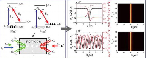
Graphical Abstract

Keywords:

• Parity-time symmetry
• coherent atomic gases
• non-linear optical effect

1. Introduction

The Hamiltonian of a quantum system, H, specifies the energy spectrum and time evolution of the system. In standard quantum mechanics, H is assumed to be Hermitian, which guarantees the energy spectrum to be real and the time evolution to be unitary (probability preserving). However, several cases of non-Hermitian Hamiltonian supporting entirely real spectrum have been known in physics for a long time, e.g. the Bogoliubov-de Gennes equations [1] or the Schrödinger equation with the potential having a parabolic real part plus a linear imaginary part [2]. In fact, spectrum of any Hermitian operator is purely real, whereas the converse is not true. That is, for obtaining all-real spectrum for an operator, the requirement of its Hermiticity is a sufficient but not necessary condition.

It was due to the work of Bender and Boettcher [3] that the fundamental importance of non-Hermitian Hamiltonian exhibiting entirely real spectrum became widely recognized. In their work, Bender and Boettcher proved that all-real spectra may appear for a broad class of Hamiltonians which are not Hermitian but invariant under the transformations of parity () and time () inversions, i.e. symmetry. The parity inversion operator P and the time reversion operator T are defined, respectively, by (1a) where is any wave function in quantum mechanics. One can verify that , where I is the identity operator, and . In terms of the P and T operators, if a Hamiltonian is symmetric, the PT operator commutes with H, i.e.(1b)

When a simple one-dimensional system is described by the Hamiltonian with a complex potential V(x), reading as(2)

where U(x) and W(x) are real functions, the system is symmetric as long as the condition , i.e. U(x) is an even function [ ] and W(x) is an odd function [], is satisfied.

A deep connection between symmetry and the reality of the spectrum of the Hamiltonian H was pointed out by Bender and his coworkers [3,4], who also introduced the concept of unbroken and broken symmetry. Since the PT operator is not a linear one, the eigenstate of H may or may not simultaneously be the eigenstate of PT. Thus, unlike Hermiticity the Hamiltonian H having a symmetry is not sufficient for its spectrum to be purely real. However, it becomes sufficient when combined with the requirement that the symmetry is unbroken. Particularly, the symmetry of a -symmetric operator H is said to be unbroken if any eigenfunction of H is simultaneously the eigenfunction of the operator. If the unbroken symmetry does not hold, the broken symmetry will result in the presence of complex eigenvalues, i.e. at least a pair of real eigenvalues coalesce and bifurcate into complex plane. The -symmetry breaking and the associated change from real to complex eigenvalues can be generally observed when the gain or loss of the system under consideration is changed. On the other hand, unlike Hermiticity symmetry does not ensure the completeness of eigenfunctions. That is, even if the spectrum of a -symmetric operator is entirely real, the set of its eigenfunctions may not constitute a complete basis. More details about the relation between symmetry and Hermiticity can be found in Ref. [5]. A nice and comprehensive review on the symmetry and its applications in non-Hermitian quantum mechanics and quantum field theory has been illustrated in detail by Bender (see Ref. [6]).

Although the concept of symmetry was initially motivated by the development of quantum theory [3,4,6], it was soon extended to various research branches of physics, including optics [7–11], plasmonics [12,13], atomic physics (especially Bose–Einstein condensation of ultracold quantum gases) [14–19], acoustics [20,21], and electrical circuits [22]. In particular, due to the similarity between the Schrödinger equation in quantum mechanics and the Maxwell equation in electromagnetic theory under paraxial approximation, optics provides a fertile ground where -related concepts and research results can be realized and tested experimentally. In optics, the complex refractive-index distribution of a medium, n(x), plays the role of the potential V(x) in Equation (3(3) ) (where x represents the transverse coordinate). Then, an optical potential is -symmetric means the requirement(3)

i.e. the real part of the index profile Re[n(x)] must be even function while its imaginary part Im[n(x)] (denoting loss or gain) must be odd function of x. A detailed review on periodic optical potentials with symmetry has been given in Ref. [23]. Due to the significant progress achieved in recent years by developing optical materials with different functionalities, the theoretical results of -symmetric optical theory were soon confirmed in a series of experiments using optical waveguides [24–26], synthetic photonic lattices [27,28], optical microcavities [29,30], and multi-level atomic gases [31–38], and so on. Such investigations have also led to many attractive practical applications, such as the realization of nonreciprocal and unidirectional invisible light propagations [26,39–41], coherent perfect absorbers [42–45], giant light amplification [46], novel lasers [47,48], and so on.

On the other hand, developments in -symmetric optics suggested further extension of theory to include non-linear effect, which is inherent in many fields of physics and is responsible for a wide variety of new phenomena. In this line, the study was initiated in non-linear optical systems with linear -symmetric potentials [10]. Later on, optical systems with non-linear -symmetric potentials [49] and with mixed linear and non-linear -symmetric optical lattices [50] were also suggested. Non-linear effects for light-beam dynamics in various optical systems with -symmetry were also investigated, including optical couplers, optical waveguides [51–57], oligomers [58–60], 2D plaquettes [60,61], finite/infinite chains [62–65], necklaces [66], and multi-core fibers [67], etc. As the research further develops, the possibility of non-linear excitations, especially optical solitons, in different types of -symmetric structures [68–89] were studied. Other non-linear phenomena such as four-wave mixing was also explored in -symmetric couplers [90]. Two comprehensive reviews on non-linear -symmetric systems have been provided by Konotop et al. [91] and by Suchkov et al. [92] recently.

Among the various -symmetric optical systems, -symmetric coherent atomic gases possess many unique features. First, they have authentic -symmetric refractive index, which has balanced gain and loss in the whole space. Second, they can be actively controlled and precisely manipulated by changing the system parameters in situ. Third, because usually working in regimes of resonance between light and atoms, they are inherently highly non-linear, and hence one can acquire symmetric optical systems with enhanced non-linear optical effects.

We recall that, in the development history of non-linear optics, attempts to use resonances to enhance optical nonlinearity have long been hampered by serious optical absorption. However, this paradigm has been challenged by recent theoretical and experimental studies on coherently driven atomic systems with electromagnetically induced transparency (EIT) [93]. By means of the destructive interference induced by a control laser field, the absorption of a probe laser field can be largely suppressed and hence an initially highly opaque optical medium becomes transparent. As a result, enhanced optical nonlinearity with eliminated absorption can be achieved in the systems via EIT [94]. Besides EIT-related systems, the systems with Raman resonances (i.e. all laser fields are far off the one-photon resonances but close to the two-photon resonances) can also exhibit enhanced optical nonlinearity with a small absorption. Due to these reasons, the coherent atomic gases driven by laser fields designed to be -symmetric may be served as powerful building blocks for developing novel non-linear photonic devices that can be actively controlled and manipulates at very low power level.

In this article, we present a comprehensive introduction on the recent development of the symmetry in coherent atomic gases. We review different physical schemes for the realization of symmetry via laser-driven multi-level atomic gases. The interesting physical properties and promising applications of -symmetric atomic systems are discussed, and several experiments carried out for demonstrating the symmetry with coherent atomic gases are also described. Finally, perspectives on the further study of the symmetry using coherent atomic gases are given.

2. -symmetric optical potentials: three-level atomic model

A mixture of two isotopes of three-level atoms with -type configuration was firstly used for attaining a large index of refraction with vanishing absorption [95–98]. The essential idea of such system is to establish two Raman resonances, one of which results in gain and another in absorption, and hence the real (imaginary) part of the susceptibility appears as an even (odd) function of the probe-field frequency. Since for a monochromatic beam the change can be viewed as a time inversion symmetry , the system can have -symmetric refractive index. Such scheme was firstly proposed by our group [31,34–36] using a three-level atomic system coupled with two laser fields.

2.1. The 3-level atomic model

The physical setting under consideration consists of an atomic gas with two isotopes, say Rb (species 1) and Rb (species 2), as shown in Figure 1(a). Each isotope is represented by a three-level configuration with two ground-state sublevels and , and one excited state ( indicates the specie of the atoms). A weak probe field and a strong control field , propagating along the z-direction with wavenumbers and , couple ground-state sublevels and to excited level , respectively. For the mixture of rubidium isotopes one can assign , , and . The half Rabi frequencies of the probe and control fields are and , respectively. Here () represents electric dipole matrix element associated with transition from to ( to ), which is assumed to be approximately equal for both isotopes. For selected levels of rubidium atoms, the electric dipole matrix element is Ccm [99].

Figure 1. Three-level atomic model for realizing symmetry. (a) Energy-level diagram and Raman scheme of the mixture of two three-level systems. and are weak probe field and strong control field, respectively. () and are one- and two-photon detunings, respectively. The initially populated levels (i.e. and ) are indicated by black dots. (b) Possible experimental settings for the suggested system. is the far-detuned Stark field. The control (Stark) field consists a z-direction laser beam, (), and two pairs of laser beams, () (, 2), with the same cross angle (). Source: Adapted from Ref. [31,36].

Under electric dipole approximation (EDA) and rotating-wave approximation (RWA), the Hamiltonian of the system in interaction picture is given by , where H.c. denotes Hermitian conjugate, is the one-photon detuning and is the two-photon detuning, with being the eigenfrequency of the level . All fields are far off the one-photon resonance but close to the two-photon (Raman) resonance, which implies that . Each isotope is initially prepared in one of the two ground-state sublevels via optical pumping as indicated by black dots in Figure 1(a). The first isotope exhibits two-photon absorption while the second isotope exhibits two-photon gain for the probe field.

The motion of atoms is governed by the Bloch equation [100] (4) where ( for ; for ), , and . Here, and are, respectively, the spontaneous-emission decay rates from the excited state to two ground-state sublevels and , assumed to be approximately equal for the both isotopes. Within the required accuracy, one can take . The decay rate from to is about four orders smaller than , and hence can be safely neglected. Since the isotopes are loaded in a cell at low temperature, the decay rate  MHz for Rubidium atoms [99]. In addition, the two-photon detuning of the second isotope can be taken as zero, i.e. , which can be achieved by tuning the frequency of the probe field .

The susceptibility of the probe field is defined by , where is the density of the s-th isotope and the coherence can be computed from the Bloch Equation (5). Assuming , one can employ the expansions (), where is of order of . Substituting the expansions into the Bloch Equation (5) and neglecting the derivative with respect to time, Equation (5) in the leading order are solved by and , with other leading elements of the density matrix being zero. In higher orders, we obtained the recurrent equations (5a) where . Equation (6) can be solved order by order.

The expression of coherence up to the third order was explicitly computed in Refs. [34–36], allowing to express the probe-field susceptibility in the form of , where the first- and third-order susceptibilities, and , are, respectively, given by(5b)

with . When obtaining (8(8) ), the assumptions and is used, which corresponds to a realistic choice of the system parameters given below.

The spatial distribution of the -symmetric probe-field susceptibility, [and hence the -symmetric refractive index ], is obtained by applying a far-detuned laser field (i.e. the Stark field), , which induces shifts of levels , i.e. (here is the scalar polarizability). In addition, the control field is assumed to be x -dependent, . For the selected levels of rubidium atoms, Hz(cm/V) and [99]; this means the difference of the Stark shifts between the ground-state sublevels is negligible, i.e. the two-photon detunings are not affected by the Stark field , while the one-photon detunings become x-dependent, . Hence, one has and .

The equation of motion for the probe-field Rabi frequency can be obtained using the Maxwell equation , where the polarization intensity of the probe field is given by . Under paraxial approximation and slowly varying envelope approximation (SVEA), we have(5c)

where the scaled variables and (, with being the wavelength of the Stark field). Here, for simplicity, is assumed to be independent on y, which is valid only for the probe beam having a large width in the y-direction so that the diffraction term can be neglected.

The first-order susceptibility can be expressed as , where and are, respectively, the constant and modulated parts of . With given parameters, is two orders smaller than , i.e. . Using the transformation (where b is the propagation constant and is the typical Rabi frequency) and preserving the terms up to the third order (-order), Equation (9(9) ) can be written into(5d)

where is the optical potential, given by , is the non-linear coefficient characterizing Kerr nonlinearity, given by , and is the eigenvalue, given by .

2.2. -symmetric Scarff II potential and weak-light solitons

Since the system described above can be easily manipulated, we can obtain different types of optical potentials obeying symmetry [31,34–36]. The susceptibility function we need is of the form , referred as the target susceptibility function, where and are, respectively, the real and imaginary parts of . symmetry requires and . At , the susceptibility must be real, i.e. . Thus, when the values of and are given at , denoted as and , the value of () can be determined by the equation , and the solution is . Further, can be determined by the equation .

The probe-field susceptibility is a function of and . Expanding it around and gives (5e) where (5f) Since , to determine the profiles of and we can solve the equations (6a) Once is obtained, we can further compute the profile of through.

The error of this method originates from the neglected higher order terms in the Taylor expansion, mainly the second-order terms. Thus the condition (6b) must be satisfied to make sure that the error is negligible. Otherwise, one needs to take into account the second-order terms in the expansion. Moreover, by tuning and it is possible to control the system to work above or below the exceptional point (see the following examples).

To prove the effectiveness of the above method, we consider a single -symmetric potential, corresponding to the Scarff II potential [101], i.e.(7)

with and being the amplitudes of the real and imaginary parts. The linear problem associated with Equation (10(10) ) and the potential (15(15) ) exhibits the entirely real spectrum provided that . Thus for a fixed value of , there exists a threshold for the imaginary amplitude , above which a -symmetric phase transition occurs and the spectrum enters the complex domain. In the non-linear regime, the refractive-index distribution can be modified by the beam itself through the nonlinearity, and hence stable solitons may exist even if the -symmetric potential has crossed the phase transition point.

In what follows, the values of detunings are taken to be , , and . Atomic densities of the first and second isotopes cm and cm, respectively. With these parameters, we can obtain the Scarff II potential (15(15) ) by the first-order probe-field susceptibility(8)

which can be realized using the control and Stark fields shaped as(9) (10)

with V cm. Notice that Equation (16(16) ) gives the order of small parameter and hence defines the accuracy of the expansion. From Equations (17(17) ) and (18(18) ) one can estimate the powers required for the control and Stark fields, which are given by V cm ( Hz) and V cm, respectively. Being focused into a spot with radius  mm, this requires laser power mW.

Figure 2. -symmetric Scarff II potential and soliton solutions. (a) Real (solid line) and imaginary (dashed line) parts of the refractive index . (b) Control (solid line) and Stark (dashed line) fields required for the refractive index, and . (c) Real (solid) and imaginary (dashed) parts of the soliton amplitude for and . (d) Evolution of the soliton solution (19(19) ) after adding random noises on both amplitude and phase.

Shown in Figure 2(a) are the real and imaginary parts of the refractive index . The potential parameters used are and , which is below the phase transition point. The control and Stark fields required for the -symmetric refractive index are plotted in Figure 2(b). For estimating the accuracy of the refractive-index symmetry, we define the error function defined by . Its real and imaginary parts are of order of and , respectively. Thus, very high accuracy of the refractive-index symmetry is obtained.

The third-order probe-field susceptibility can be computed using Equation (8(8) ). In general, the real and imaginary parts of depend on the spatial coordinates and violate the symmetry. These effects, however, are two orders smaller than its main (constant) part, i.e. they are beyond the required accuracy and can be safely neglected. In addition, the imaginary part of is much smaller than its real part and can also be neglected. As a result, for the given parameters we obtain , which corresponds to (defocusing nonlinearity) for . Since the third-order susceptibility is largely enhanced owing to the existence of two nearly resonant Raman transitions, very weak probe-field intensity is needed for obtaining a large non-linear optical effect. This is very different from any passive optical materials where intensive laser fields are usually required for obtaining enough nonlinearity to balance the dispersion or diffraction.

Equation (10(10) ) with Scarff II potential (15(15) ) and admits an exact soliton solution with the form(11a)

for . Figure 2(c) shows the real and imaginary parts of the soliton amplitude for and . In order to check the robustness of the soliton, the solution (19(19) ) is involved using Equation (9(9) ) with the potential (15(15) ) after adding random noises on both the amplitude and phase in the soliton. The result of this simulation, shown in Figure 2(d), indicates that the soliton is stable during propagation. The optical power for generating such soliton solution may be estimated using Poynting’s vector, which gives when taking the beam radius  mm. Consequently, comparing the optical solitons produced in conventional systems [102], very low input power is needed for generating the soliton in the atomic gas given above. Note that spatial solitons and their stability in Kerr non-linear media with generalized -symmetric Scarff-II potentials was recently studied in Ref. [103].

2.3. -symmetric periodic potential and weak-light gap solitons

The second example is the complex, periodic optical potential with symmetry(11b)

In general, the band structure of a complex optical lattice potential is complex. However, for a -symmetric optical lattice potential the energy band can be entirely real as long as the system is operated below the phase transition point of symmetry breaking. For the potential (20(20) ), purely real bands are possible in the range [23].

With given parameters, the periodic -symmetric potential (20(20) ) can be realized in the coherent atomic gas with(13a)

which can be realized using the control and Stark fields shaped as(13b)

Figure 3(a) shows the real and imaginary parts of the refractive index for and , which is below the phase transition point. The control and Stark fields required for the -symmetric are plotted in Figure 3(b). The associated band-gap structure for various values of [i.e. (below the phase transition), 1.5 (on the phase transition point), and 2.25 (above the phase transition point)] is given by Figure 3(c) (real part of the energy band) and Figure 3(d) (imaginary part of the energy band). One sees that as is increased the band gap in the real part becomes narrower and closes completely when crossing the critical transition value ; the imaginary part of the energy band is zero in the whole axis for and 1.5, and is nonzero for .

Figure 3. -symmetric periodic potential and gap soliton solutions. (a) Real (solid line) and imaginary (dashed line) parts of the refractive index . (b) Control (solid line) and Stark (dashed line) fields required for the refractive index, and . (c) Real part of the ‘energy’ band for and (solid lines), 1.5 (dotted lines), and 2.25 (dashed lines). (d) Imaginary part of the ‘energy’ band for and . It is zero in the whole axis of the lattice momentum q for and 1.5. (e) Real (solid) and imaginary (dashed) parts of the soliton amplitude for . (f) Evolution of the gap soliton after adding random noises on both amplitude and phase. Source: Adapted from Ref. [36].

It is well known that stable gap solitons of bright type can be obtained in systems with a self-defocusing nonlinearity combining with a real periodic potential. This conclusion is still valid for the system with a complex periodic potential of symmetry. For Equation (10(10) ) with , we numerically constructed a family of localized soliton solution for with real eigenvalues located within the first energy gap, . The real and imaginary parts of amplitude of such a gap soliton for is shown in Figure 3(e). The evolution of the soliton, after adding random noises on both amplitude and phase to the initial condition, is given in Figure 3(f), indicating that the soliton is stable during propagation. The optical power for generating the soliton shown in Figure 3(e) and (f) is very low, given by  nW with the beam radius  mm [36]. Solitons for located within the first energy band were also considered, which, however, are unstable.

2.4. Realization of the distribution of the control and Stark fields

A simple way for producing the spatial modulation of the control and Stark fields for realizing the symmetry in the atomic system is the use of high-resolution spatial light modulators. However, since all lengths are scaled by , which is m (inside the mid-infrared spectral range) in the above examples, the pixel pitch of spatial light modulators should be much smaller than . This is a very restrict requirement as the smallest pixel pitch of spatial light modulators nowadays is m, which is still larger than .

An alternative way for realizing the spatial modulation of the control and Stark fields is to use the standing-wave light fields [31]. To obtain the control-field distribution (22(22) ), one can assume that the control field consists of three laser beams, one propagates along z-direction, i.e. , and other two propagate in x–z plane with a cross angle , i.e. , where and are, respectively, the amplitudes and phases of the j-th pair of laser beams (, 2), as shown in Figure 1(b). If is very small, i.e. and , the transverse distribution of the control field can be written as , which results into . Thus, for obtaining the control-field distribution (22(22) ), one can take , , , (), and .

The Stark-field distribution needed for realizing the symmetry can also be realized using standing-wave light fields. Assuming the Stark field consists of a laser beam propagating along the z-direction, i.e. , and two pairs of cross laser beams, i.e. [see Figure 1(b)], and choosing , , , , , and , one can obtain the Stark-field distribution (23(23) ).

3. -symmetric optical potential: 4-level atomic models

Besides the three-level atomic model described above, there are other models that may be used to realize a -symmetric optical potential. In Refs. [32] and [33], two different schemes were introduced and both of them consist of four-level atomic gases. In contrast of the three-level atomic system, the four-level ones need only one species of atoms.

3.1. The four-level atomic model with coherent optical pumping

In Ref. [32], Sheng et al. considered a four-level N-type atomic system, as shown in Figure 4(a). In their model, the signal and coupling laser fields drive the atomic transitions and , respectively; A pumping laser field driving the atomic transition provides a gain to the system. By choosing appropriate parameters, the two coupling (blue) and two pump (green) beams, which propagate in the longitudinal direction (z direction), form two coupled waveguide structures, with one providing gain and the other providing absorption. The signal (red) beam propagates in the same direction along with the coupling and pump beams, as shown in Figure 4(b). Under the rotating-wave approximation, the Hamiltonian of the system in interaction picture is given by . Here, , , and are Rabi frequencies of the signal, coupling, and pump fields, respectively; , , and are frequency detunings of the signal, coupling, and pump fields, respectively. The motion of atoms interacting with the light fields is described by the optical Bloch equation(14a)

where is the density-matrix elements in the interaction picture and is a relaxation matrix. Explicit expressions of the Bloch Equation (24(24) ) are presented in Appendix 1.

Figure 4. 4-level N-type atomic system with a coherent optical pumping. (a) The signal and coupling laser fields drive the atomic transitions and , respectively; the pumping laser field drives the atomic transition , which provides a coherent gain to the system. (b) The schematic diagram with signal (red), coupling (blue), and pump (green) fields. x and z represent the transverse and longitudinal directions of propagation, respectively. Source: Adapted from Ref. [32].

The susceptibility of the atomic medium can be obtained through the expression . Given that , and , the real and imaginary parts of the refractive index can be written as and , respectively. In addition, is the background index of the system.

In order to realize a dual -symmetric potential that allows an exchange of optical energy, one can employ two different coupling fields side by side, with each having an identical Gaussian intensity profile, while the susceptibility of the signal field varies in the transverse direction (x direction) as a function of the coupling field intensity. Since the coupling fields are from two independent lasers and the overlapped region between them is relatively small, the phase effect between them is not considered. In this case, the total spatial intensity distribution of the coupling beams is assumed to be(14b)

where A is a constant, 2a is the separation between the two potential channels and is the full width at half maximum (FWHM) of the beam width. Even though the coupling intensity profiles for these two channels are identical, by choosing different coupling frequency detunings, one can actually introduce gain in one waveguide and absorption in the other one.

To this end, one needs to identify the relation between the susceptibility and the coupling frequency detuning. Figure 5(a) and (b) show the real (dispersion) and imaginary (gain or absorption) parts of the susceptibility versus the coupling detuning for various coupling intensities, respectively. The parameters are taken as ,  MHz,  MHz, and , 1 and 0.5 MHz for black (solid), red (dashed), and blue (dotted) curves, respectively. To achieve waveguiding, the signal field is focused at the center of each potential channel that is formed by the joint action of the coupling and pump beams. Therefore, the real part of the susceptibility needs to be larger with increasing coupling intensity. For this reason, the coupling detunings should be negative. One can see that the imaginary part of the susceptibility is close to zero when the coupling detuning is about  MHz, as shown in Figure 5(b), and in the vicinity of this zero point, absorption is induced on the left side, and gain on the right.

Figure 5. (a) The real (dispersion) and (b) imaginary (gain or absorption) parts of the susceptibility versus the coupling frequency detuning. , 1, and 0.5 MHz for black (solid), red (dashed), and blue (dotted) curves, respectively. The (c) real and (d) imaginary parts of the susceptibility versus the coupling Rabi frequency. The black, solid (red, dashed) curves represent and for the gain (absorption) waveguides. The chosen parameters are and  MHz for the gain and absorption waveguides, respectively. Source: Adapted from Ref. [32].

Sheng et al. [32] took two different frequency detunings of the coupling field for simultaneously introducing gain and absorption in the two separate waveguides. This implies that the only difference between these two channels comes from the values of coupling-field detunings, while all other parameters remain identical. To achieve this goal, one needs to get the relation between the susceptibility and the coupling Rabi frequency. For example, by choosing and  MHz for the two coupling fields, the real parts of the susceptibility associated with these two waveguides overlap quite well, as shown in Figure 5(c). However, the imaginary parts for the gain and loss waveguides are not matched perfectly, as shown in Figure 5(d) (the curve for the gain waveguide is flipped by multiplying a minus sign for the black solid curve).

By choosing the full width at half maximum (FWHM) to be 7 m when the separation between the two waveguides is 20 m, the intensity-dependent index graphs displayed in Figure 5(c) and (d) can be converted into their corresponding index landscapes, as shown in Figure 6. It is clear that the real part of the refractive-index distribution is an even function of transverse coordinate x, whereas the imaginary part is odd simultaneously. The value of the refractive index can be easily modified by changing atomic density. Here, the atomic density of the system is assumed to be cm. In this case, the maximum contrast in the real part of the refractive index is in the order of . In this situation, each optical potential channel can support only one mode. In addition, one can control the ratio between the real and imaginary indices by changing the two coupling frequency detunings, which determines whether the system works below or above the threshold of -symmetry. When the coupling detuning moves away from the near zero point [ MHz], the ratio between the real and imaginary indices can be modified, and the system can operate either below [Figure 6(a)] or above [Figure 6(b)] the threshold point, or can even behave as a passive one without symmetry [Figure 6(c)]. Here, the ratio between the real and imaginary indices is , 10, and 3000, for Figure 6(a), (b) and (c), respectively. Under these conditions the threshold of the -symmetry is about 27.

Figure 6. The real (solid black curves) and imaginary (dashed blue curves) refractive indices as a function of position x for (a) below threshold, (b) above threshold, and (c) conventional Hermitian cases. The parameters used are and  MHz for the gain and loss waveguides in part (a); and  MHz for waveguides in (b); and in (c), respectively. The atomic density is cm while the other parameters are the same as in Figure 5. Panels (d)–(f) show optical beam propagation patterns for the signal beam in the index potentials of (a)–(c), respectively. Source: Adapted from Ref. [32].

The propagation of a signal beam is shown in Figure 6(d), (e), and (f) corresponding to index structures as given in Figure 6(a), (b), and (c), respectively. In the case of the -symmetric potential which operates below the symmetry breaking threshold, the light dynamics looks similar to that of a passive coupler, i.e. the optical field periodically oscillates between the two waveguides. By increasing the gain–loss contrast, transitions from stable to exponentially growing modes can occur, signifying the onset of -symmetry breaking, as shown in Figure 6(e). Finally, the propagation dynamics of the passive potential of Figure 6(c) is depicted in Figure 6(f).

Figure 7. The real (solid black curves) and imaginary (dashed blue curves) parts of the refractive index for periodic lattices as a function of position x when (a) the coupling intensity and coupling detuning are spatially modified, as well as when (b) the coupling and pump intensities are spatially modified. Source: Adapted from Ref. [32].

One can also introduce additional coupling beams in order to realize an optical lattice potential, as shown in Figure 7(a), with each waveguide channel in this lattice case filled with half gain and half loss. The ratio between the real and imaginary indices in Figure 7(a) is . Instead of using continuously varying coupling intensity and discontinuously varying the coupling frequency detuning to generate the optical lattice potentials, an alternative way is to use continuously varying coupling and pump intensities. For example, the coupling and pump beam intensities are spatially modified as cosine and sine functions, respectively, while the other parameters remain uniform in space. In such case, a -symmetric optical lattice potential can be established, as shown in Figure 7(b). The parameters used in generating Figure 7(b) are  MHz,  MHz,  MHz, and  MHz, with m being a scale factor. All the other parameters used are the same as in Figure 6. The ratio between the real and imaginary indices in Figure 7(b) is , which can be changed to be below or above the -symmetry breaking threshold by modifying the amplitudes of the sine or cosine functions. The optical lattice potential can also be extended to two dimensions (2D) when the coupling and pump intensities are simultaneously modulated in x and y directions.

3.2. The four-level atomic model with incoherent optical pumping

Almost at same time, Li and Huang also introduced a four-level scheme for realizing a -symmetric optical lattice potential [33]. The system under consideration consists of a cold, lifetime-broadened Rb atomic gas with N-type level configuration, as shown in Figure 8. Different from Ref. [32], in this model the gain of the system is provided by an incoherent optical pumping.

Figure 8. Four-level N-type atomic system with an incoherent optical pumping. (a) The probe and control laser fields drive the atomic transitions and , respectively; an incoherent pumping is used to couple the atomic transition , which provides an in coherent gain to the system. (b) Possible experimental arrangement. All the notation are defined in the text. Source: Adapted from Ref. [33].

The levels of the system are taken from the D line of Rb atoms, with , , and . A weak probe field and a strong control field interact resonantly with transitions and , respectively. Here and () are, respectively, the polarization unit vector in the xth direction and the wave number (envelope) of the jth () field.

Furthermore, an assisted filed, , is assumed to couple the transition , where is field-distribution function in the transverse direction (x direction). The assisted field, , when assumed to be weak (satisfying ), will contribute a cross phase modulation (CPM) effect to the probe field . Note that the levels () together with , and form a N-type system. In addition, another far-detuned (Stark) optical lattice field, , is assumed to be applied to the system, where and are, respectively, the field-distribution function and angular frequency. Due to the existence of , a small and x-dependent Stark shift of level to the state occurs, i.e. with , here is the scalar polarizability of the level , and denotes the time average in an oscillating cycle. The explicit forms of and are chosen in according with the requirement of symmetry.

The CPM effect contributed by the assisted field and the Stark shift contributed by the far-detuned Stark field may provide periodic complex refractive index to the evolution of probe-filed envelope. However, the system is still a dissipative one. In order to have gain in the system, an incoherent optical pumping is introduced, which can pump atoms from the ground-state level to the excited-state level with the pumping rate . Such optical pumping can be realized by many techniques, such as intense atomic resonance lines emitted from hollow-cathode lamps or from microwave discharge lamps [104].

In Figure 8(a), , and are spontaneous-emission rates denoting the population decays, respectively, from to , to and to ; , , and are, respectively, the half Rabi frequencies of the probe, control and assisted fields, where signifies the electric dipole matrix element of the transition from state to , and , and are one-, two- and three-photon detunings in relevant transitions, respectively. Figure 8(b) shows a possible experimental arrangement.

Under EDA and RWA, the Hamiltonian of the system in interaction picture reads , where h.c. denotes Hermitian conjugate, and . The motion of atoms interacting with the light fields is described by the Bloch equation(15)

where is the density-matrix elements in the interaction picture and is a relaxation matrix. Explicit expressions of Equation (26(26) ) are presented in Appendix 2, in which an incoherent optical pumping (represented by ) from the level to the level is introduced [see Equations (B1a) and (B1c)].

Under SVEA, the Maxwell equation for the probe field is reduced to(16)

where with N the atomic density. Note that, the dynamics of is assumed to be negligible during the probe-field evolution, which is a reasonable approximation because the assisted field couples to the levels and that always have vanishing population due to the EIT effect induced by the strong control field.

Because the probe field is weak, a perturbation expansion can be used for solving coupled equations (26(26) ) and (27(27) ) analytically [105–107]. To this end, the expansions and are used, with being a small parameter characterizing the typical amplitude of the probe field (i.e. ). Substituting such expansion to equations (26(26) ) and (27(27) ), one obtains a series of linear but inhomogeneous equations for and () that can be solved order by order. To get a divergence-free perturbation expansion, and are considered as functions of the multiple scale variables () and . In addition, the envelopes of the assisted field and the Stark field are assumed to be small, and are slowly varying functions in x, i.e. and . Thus, one has , with and .

At -order, one obtains non-zero density-matrix elements , , , and , with and . It can be seen that due to the existence of the incoherent optical pumping (i.e. ) there are populations in the states , , and . Because is on the order of MHz in our model, the populations in and are small. If , it is straightforward that and .

At -order, the solution is given by , , , , and , with other . Here F is yet to be determined envelope function, , , and the linear dispersion relation(17)

Because in the linear case , the real and imaginary parts of linear dispersion relation characterize, respectively, the phase-shift and gain or loss during the probe-field propagation.

Figure 9. The imaginary part of the linear dispersion relation, i.e. ImK, as a function of for . Solid (red), dashed (green), and dashed-dotted (blue) lines correspond to , ( Hz, 0), and ( Hz, ), respectively. For illustration, the value of dashed-dotted (green) line has been amplified 7.8 times. Source: Adapted from Ref. [33].

Shown in Figure 9 is ImK as a function of for . The system parameters used are [99] Hz, Hz,  MHz, and cm Hz. Solid (red), dashed (green), and dashed-dotted (blue) lines correspond to , ( Hz, 0) and ( Hz, ), respectively. From the solid line of Figure 9, one sees that in the absence of the control field and incoherent pumping (i.e. ), the probe field has a very large absorption. However, when the incoherent pumping still absent but takes the value of Hz, a transparency window is opened (as shown by the dashed line). This is well-known EIT quantum interference phenomenon induced by the control field. Notice that although EIT can greatly suppress the absorption, it cannot eliminate the absorption completely, i.e. there is still a small absorption (i.e. Im). The dashed-dotted line in Figure 9 is the situation when the incoherent pumping is introduced (). One sees that a gain, i.e. negative ImK in the region near , occurs. Such gain is necessary to attain a -symmetric optical potential for the probe-field propagation.

At -order of the perturbation expansion, the closed equation for F is obtained. When converting this equation into the one for , one has(18)

with(19)

The explicit expressions of the coefficients and are given in the appendix of Ref. [33].

The susceptibility of the probe field is then given by , and hence the refractive index . In order to realize a symmetry for the system, the spatial distributions of the assisted and Stark fields are selected to have the form and , with and being typical amplitudes and being typical ‘optical lattice’ parameter.

A -symmetric optical potential can be obtained by choosing the system parameters as , , C cm and . Other (adjustable) parameters are taken as , , , , and . Then one obtains(20)

Based on these parameters, the assisted laser field (31(31) ), the far-detuned Stark laser field (32(32) ), and the optical pumping (33(33) ), one obtains and as a result,(21)

which apparently satisfies the symmetry, exact to the accuracy . The constant term in V(x) can be removed using a phase transformation. Moreover, with the present system, it is possible to design different types of -symmetric optical potentials and manipulating them in a controllable way [33].

4. Tunable non-linear -symmetric defect modes in coherent atomic systems

Defects are known to play an important role in controlling, manipulating, and guiding lights, which relate to many useful applications. Depending on the physical nature of a defect, one can distinguish conservative and nonconservative defects, as well as linear and non-linear ones, which display very different properties with respect to the modes they support. In particular, the modes supported by non-linear nonconservative defects have been attracting increasing attention in recent years, see [108–112].

Recently, a way of implementing tunable non-linear defects in an atomic cell was suggested by our group [34,35]. Different from the previous works [108–112], the non-linear defect we studied is symmetric. The cell confines atoms in space and can be used to cut undesirable deviations from symmetry, which allows for construction of refractive indexes with different shapes, such as parabolic and double-hump shapes. Families of stable non-linear defect modes can be formed by the probe field in the atomic cell.

4.1. Tunable non-linear single-core -symmetric waveguides

Consider a one-dimensional photonic crystal with an embedded atomic cell filled by a mixture of two isotopes of cold three-level atoms [34]. Different from the system depicted in Figure 1, here corresponds to Rb while corresponds to Rb, as shown Figure 10(a). The densities for each atomic isotope are taken as cm and cm. The two-photon detunings are chosen as and .

Figure 10. Atomic system for realization of tunable non-linear single-core -symmetric waveguides and the corresponding optical potential. (a) Geometry of the photonic crystal, the energy-level diagram, and the Raman resonance scheme of a binary mixture. The notations represent the same as in Figure 1. (b) Distribution of real (solid line) and imaginary (dashed line) parts of the linear refractive index induced by the fields (35). Source: Adapted from Ref. [34].

The -symmetric profile of the susceptibility, with parabolic real part and linear imaginary part, can be achieved using the control and Stark fields shaped as (22) where () and V/cm.

With the above distributions of the control and Stark fields, and choosing the effective susceptibility for the Bragg cladding (i.e. ; this parameter can be changed [113,114]), the first-order probe-field susceptibility acquires the form(23)

where , , and . Figure 10(b) shows the real and imaginary parts of the linear refractive index of the defect. Real and imaginary parts of the error function for are of order of and , respectively. On the other hand, the system is working in the regime of weak guidance, which is ensured by the fact that . This gives the order of small parameter and defines the accuracy of the expansion. The third-order probe-field susceptibility is computed using Equation (8(8) ). With the above given parameters, one finds that inside the atomic cell (), .

With the above parameters, the probe field in the cell is described by the non-linear Schrödinger equation with a -symmetric linear potential, while outside the cell the system is described by the linear equation: (24) Here is the dimensionless field, where the typical Rabi frequency is chosen to scale out the non-linear coefficient in (37a(37a) ). In addition, , , and . For  mm (thus ), we obtained that s, , , and .

Without the non-linear term in (37a(37a) ), the stationary guided modes are determined by the eigenvalue problem , where b is the propagation constant and is the -symmetric operator, defined by , with for and otherwise. For the above parameters, we found numerically that has two isolated eigenvalues and [see Figure 11(a)] and a continuous spectrum situated on the real axis. The spectrum of is all real due to the unbroken symmetry.

The existence of the two bound states is supported by the given positive value of . Adjusting the parameters, one can change and hence the properties of the defect modes. For example, decrease (increase) of results in sequential appearance (disappearance) of isolated real eigenvalues b, meaning change of the number of guided linear modes. In particular, for no linear guided modes exists. Increase of the imaginary part of the potential eventually results in the symmetry breaking.

Passing to the non-linear case, each eigenvalue (i.e. , , etc.) gives birth to a family of non-linear modes, as shown in Figure 11(a) on the plane (U, b), where is the total energy flow. In the linear limit, , the propagation constants approach . With the decrease of b the total energy flow monotonously grows. A typical profile of a defect mode is shown in Figure 11(b), where the ‘current’ is also plotted, which is associated with the Poynting vector in the transverse direction. This current arises from the nontrivial phase structure of the non-linear modes. The mode shown in Figure 11(b) is well localized inside the atomic cell. Due to the enhancement of the nonlinearity, the generation power of the -symmetric defect modes considered above can be reduced to a nanowatt range.

Figure 11. Families of non-linear modes and their evolution in the non-linear single-core -symmetric waveguides. (a) Two families of non-linear modes bifurcating from the eigenvalues (see the text). The shaded domain corresponds to propagation constants belonging to the continuous spectrum. (b) The amplitude |u| (solid line) and the current S (dashed line) for the non-linear mode with . The shaded domain corresponds to the cladding. (c), (d) Evolution of the non-linear mode intensity for the -symmetric (c) and non--symmetric (d) refractive indexes. Source: Adapted from Ref. [34].

To examine stability of the mode, small (5%) random perturbations are added to both the amplitude and phase of the stationary solution, with the result shown in Figure 11(b). The calculation is done using Equation (37). One sees that the mode is robust during propagation, as shown in Figure 11(c). For comparison, in Figure 11(d) the evolution of the same input beam is repeated after decreasing by 5% without changing other parameters. In this case, the system violates symmetry and the decay of the mode appears in a relatively short distance.

4.2. Tunable non-linear double-core -symmetric waveguides

In the work [35], the spatial distributions of the control and Stark fields (25) and the effective susceptibility for the Brag cladding [113,114] (i.e. ), were chosen. Then the first-order probe-field susceptibility acquires(26)

where , , and . Figure 12(b) shows the real part () and imaginary part () of the linear refractive index n of the system. Real and imaginary parts of the error function for are of order of and , respectively. In addition, the system is working in the regime of the weak guidance, , it requires .

Figure 12. Atomic system for realization of tunable non-linear double-core -symmetric waveguides and the corresponding optical potential. (a) Excitation scheme of the binary mixture of -type three-level atoms [Rb (species 1) and Rb (species 2)] filled in a cell embedded in a 1D photonic crystal waveguide. (b) Real part () and imaginary part () (solid and dashed lines) of the linear optical refractive index n induced by the control and Stark fields (38). Source: Adapted from Ref. [35].

The third-order non-linear optical susceptibility of the probe field inside the atomic cell () can be computed using Equation (8(8) ). For the above-mentioned parameters we got cm V. Note that, in contrast to the defect studied in the last subsection, where defocusing nonlinearity was produced, here a focusing nonlinearity is obtained. In this case, the defect may support bound states even if the linear potential maintains only extended states [115,116].

With the above results, the equation for the propagation of the dimensionless probe-field envelope reads(27)

For  mm (thus, ) and s, we had , and .

In the linear limit of Equation (40(40) ), the energy levels of the system are determined by the Schrödinger operator , where is a potential well, i.e. for and for , see Figure 13(a). For the system parameters defined above the potential has two discrete eigenvalues and a real continuous spectrum, and hence symmetry is unbroken.

Figure 13. Families of non-linear modes in the non-linear double-core -symmetric waveguides. (a) Real part Re(U) (solid line) and imaginary part Im(U) (dashed line) of -symmetric double-well potential . Two lowest energy levels and are shown by red lines. (b)–(d) Total power P as a function of b for different parameter sets when the focusing nonlinearity is taken into account. Stable and unstable non-linear modes correspond to the solid and dashed curve fragments, respectively. The shaded domains correspond to propagation constants belonging to the continuous spectrum. is taken as in (b). The dots labeled by ‘A’– ‘D’ in (b) correspond, respectively, to the modes for , (2.1, 3.2), (4, 7.3), and (4, 5.7). Source: Adapted from Ref. [35].

The non-linear behavior was investigated for searching stationary modes with propagation constant b as . Figure 13(b) shows that two isolated eigenvalues corresponding to two energy levels of the linearized system [Figure 13(a)] give birth to two families of non-linear modes. These two families eventually merge at . The left family (with higher power) is stable almost up to the merger point, while the right one (with lower power) is stable for and is unstable otherwise. Thus, one can observe two stable non-linear modes with the same propagation constant for .

The evolution of these non-linear modes is illustrated in Figure 14. The left panels of Figure 14 show the real and imaginary parts of u for the non-linear modes corresponding to the dots ‘A’–‘D’ in Figure 13(b). Each mode has two humps and is well localized inside the atomic cell. To examine the non-linear stability of these modes, we added small () random perturbations to both real and imaginary parts shown in the left panels, and evolved them according to Equation (40(40) ). The results are given in the right panels of Figure 14. Notice that the first three rows show the stable non-linear modes, corresponding to ‘A’–‘C’ in Figure 13(b), respectively. The last row shows the unstable non-linear mode, corresponding to ‘D’ in Figure 13(b).

Figure 14. Evolution of the non-linear modes in the non-linear double-core -symmetric waveguides. (a)–(d) Real part Re(u) (solid line) and imaginary part Im(u) (dashed line) for the non-linear modes corresponding to ‘A’–‘D’ in Figure 13 (b), respectively. Corresponding intensity evolutions are given in (e)–(h). Source: Adapted from Ref. [35].

5. Applications of tunable -symmetric optical waveguides

The tunable PT-symmetric optical waveguides described in the last section may facilitate various applications, such as optical diode, switch, and amplifier [117]. In particular, the transitions between different guiding regimes can be achieved by a change of the effective refractive index along the propagation direction. To this end, the probe-field susceptibility can be modeled as(28)

where the expansion coefficients () are now functions of . Then, far from the transition, where the parameters of the waveguide are constant or change very slowly, one can look for a stationary mode in the form of , where could be found from solution of the eigenvalue problem , with(29)

In Ref. [117], two implementations of such a transition were presented: (i) The transition changes the number of modes supported by the waveguide, but symmetry of the entire configuration remains unbroken. For instance, an initially two-mode waveguide can undergo a transition to a one-mode or a three-mode region; (ii) The transition breaks the symmetry, i.e. several propagation constants become complex. This situation resembles recently studied interaction of a soliton in -symmetric coupled non-linear Schrödinger equations with localized coupling defect [118], as well as soliton interaction with a -symmetric localized dissipative defect [119].

5.1. Transitions between one-mode and two-mode waveguides: optical diodes and switches

The possibility of the transition between two-mode and one-mode regions can be achieved by decreasing the peak value of the real part of the refractive index, i.e. by decreasing of the parameter . As shown in Figure 15(a), for sufficiently large (say, ) the waveguide supports exactly two real isolated eigenvalues and the continuous spectrum which occupies the real semi-infinite interval . At the lowest propagation constant merges with the continuous spectrum. For small (say, ) the system has only one isolated eigenvalue and the continuous spectrum. Notice that for all values of the parameter addressed in Figure 15(a), the symmetry of the waveguide remains unbroken, i.e. all propagation constants remain real even after the transition from the two-mode to the one-mode region.

Figure 15. (a) Transition from two-mode regime to one-mode regime through the decrease of the parameter . One of the isolated eigenvalues enters the continuous spectrum for . The shaded domain is occupied by the eigenvalues from the continuous spectrum. (b) Exceptional point and transition to the broken symmetry by the increase of the parameter . Real (top) and imaginary (bottom) parts of the two isolated eigenvalues are illustrated. Source: Adapted from Ref. [117].

In the study, and are fixed, and the variation of the coefficient between two values are considered, which correspond to one-mode and two-mode regions of the waveguide. More specifically, the following model of the transition(30)

is chosen, where is the amplitude of the variation of the potential, and and are the center and width (steepness) of the transition between the two domains, respectively. In particular, large values of correspond to the slow (adiabatic) transition, while small produces the fast (non-adiabatic) transition. At the input of the waveguide (i.e. at ), one has , while at the output of the waveguide (i.e. at ), one has . Thus by choosing different values of one can design a transition between different guiding regions, for instance, a transition from the two-mode region to the one-mode region or vice versa.

When the light propagates from the one-mode region toward the two-mode one (as the first numerical experiment), there is no significant decay of the transferred power because after passing the transition the light will be arrested by two modes enhancing transparency of the waveguide. On the other hand, when the light is transmitted from the two-mode region toward the one-mode one (as the second numerical experiment), there is a significant energy transfer from the guided mode to the continuous spectrum and a significant decay of the output field in the waveguide due to the diffraction.

The results of both numerical experiments are presented in Figure 16. The first simulation was performed with the input mode, i.e. the one-humped mode [see the red solid line in Figure 16(b)], applied to the one-mode side of the waveguide. The parameters are taken as , (adiabatic transition), and . As expected, one can observe the almost complete transmission of the beam, as illustrated in Figure 16(a). After the transition, the beam is adiabatically and almost completely transformed into the two-humped mode, shown by the black solid line in Figure 16(b).

Figure 16. Propagation of a beam in waveguides with transitions between one-mode and two-mode. (a) Propagation of a beam applied to the one-mode side of the waveguide. (c) Propagation of a beam applied to the two-mode side of the waveguide. (b) and (d) the spatial profiles of the input (red lines) and output fields (back lines) corresponding to (a) and (c) at , respectively. For the first row , , and . For the second row , , and . Source: Adapted from Ref. [117].

The second simulation was performed with the input mode, i.e. the two-humped mode [see the red solid line in Figure 16(d)], applied to the two-mode side of the waveguide. The parameters are the same with those used in the first simulation, except . As expected, one can observe the almost complete diffraction of the beam, as illustrated in Figure 16(c). After the transition, the beam diffracts and attenuates rapidly, shown by the black line in Figure 16(d).

Comparing the upper and lower panels in Figure 16, one can observe the nonreciprocal propagation of the light applied to opposite sides of the waveguide with the transition between one-to-two mode configuration. Thus, the structure operates an optical diode-like device allowing for a transmission of a beam localized near the core of the waveguide in only one direction.

The adiabaticity of the transition between the two domains of the waveguide does not appear to be important for the implementation of the diode-like behavior. In order to confirm this, which can be useful to reduce the size of the device, we studied the ‘non-adiabatic’ transition between one-mode and two-mode regions by decreasing (say, ). The result is given in [117].

The unidirectional light propagation described above can also be observed if the modification of the structure of the waveguide is implemented only in a finite region of the propagation distance in the form of a localized defect. Particularly, there are two cases could be considered. In the first case, the regions outside the defect are characterized by the refractive index supporting only one mode, while the defect supports two modes. In this case, the input light remains localized after the interaction with the defect no matter the width of the defect is small or large compared with the width of the incident pulse. In the second case, the situation is inverse, where the outside regions are characterized by the refractive index supporting two modes, while the defect supports only one mode. In this case, the input light remains localized only if the width of the defect is much small than the width of the incident pulse. By increasing the width of the defect, a strong diffraction of the input light appears after it interacting with the defect. Thus, one can control the width of the defect to increase or to decrease the light intensity at the output. Namely, by increasing the defect width one can effectively decrease the light intensity, which can be viewed as ‘switching off’ the light. On the contrary, by decreasing the defect width one can preserve almost all light in the guiding mode, which can be viewed as ‘switching on’ the light.

5.2. Scattering by -symmetry breaking defects: optical amplifiers

The second implementation of the transition, i.e. the scattering of light beam by a defect, which locally breaks the symmetry, was also investigated. In order to observe this scenario, where both guided modes become unstable when passing through an broken -symmetric defect, the imaginary part of the potential (i.e. ), is increased. At the phase transition point, the two isolated eigenvalues coalesce forming a double eigenvalue. Upon the further increase of the gain-and-loss, the double eigenvalue splits into a pair of the complex conjugated ones which manifest the spontaneous breaking of symmetry. This scenario is illustrated in Figure 15(b), where the phase transition point corresponds to .

In order to model the above situation,(31)

is taken, with and (i.e. at the input and output of the waveguide, and at the center of the domain with the broken symmetry at ). The half-width of the defect, Z, is considered as a control parameter.

Figure 17. Scattering by -symmetry breaking defects. (a)–(c) Scattering by a -symmetry breaking defect for , 2, and 4, respectively. A periodic energy transfer between the two cores is clearly observed. (d) The total power P (solid line), the guided power (dash-dotted line), and the diffracted power (dashed line) as functions of the defect width 2Z. Source: Adapted from Ref. [117].

Figure 17 presents the numerical results of the described system. Panels (a)–(c) show the dynamics for three different widths of the defect. The initial condition is chosen as an eigenmode with and the propagation constant . After the beam passes the first transition and enters the region with the broken- symmetry, the light intensity grows exponentially. This growth stops after the beam passes the second transition and returns to the region with the unbroken- symmetry. The periodic energy transfer between the two cores is clearly observed due to the nonorthogonality of the modes. The output intensity grows exponentially with the distance between two transitions, as shown in Figure 17(d). Here the increase of the total power and of the power in the guided mode can be observed. However, the power in the diffracting wave increases much slower. Thus, one can control the width of the defect to amplify the light intensity at the output, i.e. the waveguide can operate as an amplifier of the beam.

6. Experimental observations of symmetry with coherent atomic gases

Inspired by the theoretical investigations on symmetry in coherent atomic gases, a few of experimental observations have been reported very recently. The first experimental observation was reported by Peng et al. [37] on the anti- symmetry with flying atoms in a warm atomic cell. In contrast with a -symmetric Hamiltonian, which obeys the commutation relation (2(2) ), an anti--symmetric Hamiltonian follows the anti-commutation relation . Then, a -symmetric Hamiltonian would become anti--symmetric on multiplying by ‘i’, implying properties of -symmetric systems conjugate to those of anti--symmetric systems. Anti- symmetry can also display many intriguing features, such as spontaneous-phase transition of the scattering matrix, a flat total transmission band, and a continuous lasing spectrum [120], which may open up new opportunities for manipulating light and form a complementary probe in non-Hermitian optics. Soon after the first experimental observation, the second one was reported by Zhang et al. [37], where symmetry was eventually realized and verified in a four-level N-type coherent atomic system.

6.1. Observation of anti- symmetry with flying atoms

In Ref. [37], Peng et al. experimentally studied the anti- symmetry with flying atoms in a warm atomic cell. The experiment [schematically shown in Figure 18(a)] was carried out in a Rb vacuum vapor cell of cylindrical shape. The inner surface of the cell is coated by coherence-preserving paraffin and the temperature is set at 40 C. The cell is housed within a four-layer magnetic shield to screen out the ambient magnetic field. Inside the shield a solenoid is used to generate a uniform magnetic field, inducing a Zeeman shift to the two-photon detuning. The laser beam, derived from an external cavity diode laser operating at the Rb D line (795 nm), is spatially split into four beams using half-wave plates and polarization beam splitters (PBS). Orthogonally linearly polarized probe and control beams are recombined, converted to circular polarization by quarter-wave plates (QWP), and directed into two optical channels, Ch1 and Ch2, separated transversely. In the first experiment [Figure 18(b)], two right-circularly polarized strong-control fields are resonant with the transition , and two left-circularly polarized weak-probe fields are nearly resonant with , but frequency shifted in opposite directions by the same one-photon detuning using acousto-optical modulators (AOMs). In each channel, the co-propagating probe and control fields set up the standard -type EIT effect and create a long-lived ground-state coherence. The two spin waves are naturally coupled through the ballistic motion of Rb atoms in the cell, where the randomness and irreversibility in the motion lays the foundation of the non-Hermiticity of the effective Hamiltonian.

Figure 18. Atomic system for realizing anti- symmetry. (a) Schematic of a three-dimensional view of the system. Two spatially separated optical channels (Ch1 and Ch2) each contain collinearly propagating weak-probe and strong-control fields operating under the condition of EIT. Output probe transmission spectra are measured by sweeping a homogeneous magnetic field generated by a solenoid inside the shield. PD, photodetector. (b) The implementation of anti- symmetry using standard three-level -type EIT configurations in two channels. An external cavity diode laser provides the light for the probe and control fields with orthogonal circular polarizations. Right-circularly (left-circularly) polarized strong-control (weak-probe) fields, and ( and ) in Ch1 and Ch2 are, respectively, resonant with ( ). and are detunings. The population is mainly in the ground state . Source: Adapted from Ref. [37].

The time-dependent non-Hermitian Hamiltonian is obtained to govern the dynamics of the two collective spin-wave excitations:(32)

Here, I is a identity matrix, , with the dephasing rate of the ground-state coherence, the ground-state-coherence coupling rate between the two channels, and the total pumping rate by the two control beams with the same Rabi frequency , where is the atomic optical coherence decay rate. The resonance condition of the coupled system is met when Det[]=0, whose solutions, coinciding with the two eigenvalues of H, define the appearance of the two eigen-EIT supermodes. is a parameter that is swept to extract the eigenvalues of H. The eigenvalues of H corresponding to the two eigen-EIT supermodes are(33)

Here, the real parts of correspond to the resonance centers of the two coupled-EIT eigenmodes and the imaginary parts represent their linewidths. Since H satisfies (i.e. ) in contrast to (i.e. ) for conventional symmetry, H is an anti--symmetric Hamiltonian. In addition, this Hamiltonian leads to an intriguing phase transition exhibited on the two eigen-EIT spectral branches. Specifically, in the symmetry-unbroken regime (), the two eigen-EIT resonances coincide at the center , but with different linewidths. The anti- symmetry breaking occurs at the exceptional point , where the two supermodes perfectly overlap. When , the driven system enters the symmetry-broken regime, and the resonances bifurcate and exhibit level anti-crossing, resembling a passively coupled system.

The spectral profiles of the two eigen-EIT spectra were experimentally probed by slowly sweeping the magnetic field with time and measuring the weak-probe transmission. Therefore, the measured probe transmission is a function of both (lower x-axis) and time (upper x-axis), as shown in Figure 19(a1), (a2) and (b1), (b2). Figure 19 shows two sets of representative probe transmission spectra with Hz [Figure 19(a1), (a2)] in the symmetry-unbroken regime and Hz [Figure 19(b1), (b2)] in the symmetry-broken regime. From the beating spectra, one can extract a set of EIT spectra, as denoted by the red/blue dots. The spectra are fitted (red/blue lines) by a weighted sum of the two eigen-EIT spectra to give the linewidth and line center values as predicted by Equation 46(46) . As one can see, both the experimental EIT spectra with the beat and the extracted spectra show good agreement with the corresponding theoretical simulations (insets).

Figure 19. Transmission spectra of output probe light in anti- symmetry. (a1), (a2) Transmission spectra of output probe light after Ch1 and Ch2 in the regime of anti- unbroken phase. (b1), (b2) Transmission spectra of output probe light with probe detuning Hz in Ch1 and Ch2, respectively, in the regime of broken anti- phase. The bold, dotted curves in (a1), (a2), (b1), (b2) are the EIT spectra extracted at time points, and the beating notes marked in dark blue are for the phase reference. The insets are calculated curves from the theory. (a3), (b3) Comparison of the dotted curves in Ch1 [(a1) and (b1)] and Ch2 [(a2) and (b2)] plotted together. (a4), (b4) Uncoupled EIT spectra separately measured from Ch1 with both channels?? control and only Ch1’s probe input on, and from Ch2 with both channels’ control and only Ch2’s probe input on. Source: Adapted from Ref. [37].

For Hz, the two eigen-EIT spectra [Figure 19(a3)] coalesce at , while for Hz, the two spectra [Figure 19(b3)] are pulled closer to each other without complete overlap, compared to the uncoupled EIT spectra [Figure 19(a4) and (b4)] separately measured from Ch1/Ch2 with both control fields on but only Ch1’s/Ch2’s probe on.

The evolution of the anti- supermodes is carefully examined by varying . The extracted line centers and their corresponding linewidths are plotted as a function of in Figure 20, showing excellent agreement with theoretical predictions. Remarkably, the current system has high resolution of the phase-transition threshold at the Hz level, which may open up new avenues for precisely measuring the optical phase or the magnetic field.

Figure 20. Anti- supermodes in coupled-EIT channels. (a), (b) Characteristics of the real part Re[] (a) and imaginary part Im[] (b) of the two eigenfrequencies of the coupled-EIT supermodes as a function of the probe detuning . The data points are obtained from curve fitting the measured transmission spectra to the theoretical result. In (a), as a comparison, the blue squares represent the EIT peak separation between two uncoupled channels, and the red dots are for the coupled case with both Ch1 and Ch2 on. In (b), the green dots and blue squares are the extracted linewidths of the two eigen-EIT modes, respectively. The error bars are standard deviations obtained from 10 measurements. The experimental parameters here are the same as those in Figure 19. Source: Adapted from Ref. [37].

6.2. Observation of symmetry in optically induced atomic lattices

Later the same year, an experimental observation on symmetry in a coherent atomic system was reported by Zhang et al. [38] Figure 21(a) schematically depicts the setup they used in the experiment. The signal field and two sets of standing-wave fields propagating along the same longitudinal z direction interact with an N-type four-level Rb atomic system [see Figure 21(b)], which consists of two hyperfine states (level ) and () of the ground state and two excited states () and (). Two elliptical-Gaussian-shaped coupling beams and (of wavelength nm, frequency , and Rabi frequencies and , respectively) from the same external cavity diode laser are symmetrically placed with respect to the z axis and intersect at the center of the rubidium cell at an angle of to establish an optical lattice along the transverse direction x inside the cell. Similarly, two pump beams and ( nm, , and and ), partially overlapped with and , respectively, enter the cell at almost the same angle to form a pump-field optical lattice. The 7 cm long atomic vapor cell wrapped with -metal sheets is heated by a heat tape to provide an atomic density of cm at 75 C. The signal beam ( nm, and ) with a Gaussian intensity profile propagates through the two sets of optical lattices, as shown in Figure 21(c).

Figure 21. Four-level N-type atomic vapor for realizing symmetry. (a) Experimental setup. and are pump beams from the same laser, and so are the coupling beams and . The reference beam intersects with to generate the reference interference. (b) The energy-level diagram of the four-level N-type configuration in Rb atomic vapor. (c) The spatial arrangements of the signal field, coupling-field lattice and pump-field lattice. x and z represent the transverse and longitudinal directions of beam propagation, respectively. marks the displacement between the two lattices. Source: Adapted from Ref. [38].

By properly adjusting the experimental parameters, the desired periodic gain and loss profiles along the x direction are obtained after passes through these two partially overlapping optical lattices. The periodically gain- and loss-modulated then interferes with a reference beam (injected in the y direction) to exhibit the induced phase difference between the adjacent gain and loss channels. The reference beam originates from the same external cavity diode laser as and is introduced into the optical path via a 50/50 beam splitter to intersect with at the position of a charge coupled device (CCD) camera [see Figure 21(a)], which is used to monitor both the output signal beam and the relative phase difference. Figure 21(c) shows a schematic diagram of the spatial arrangement for the two sets of optical lattices and inside the cell. The spatial periodicity of the coupling lattices is m, and the spatial-shift distance between the two lattices can be adjusted to control the real and imaginary parts of the susceptibility experienced by .

For a non-Hermitian gain- and loss-modulated array, the behaviors of its eigenvectors can be captured by the changes in the relative phase difference (which represents the internal phase difference of the eigenvectors) between the adjacent gain and loss channels [25]. The distance (along the y direction) between the adjacent interference fringes [as shown in Figure 22(a)] is defined as . The dotted black line gives the center of the two solid lines, so the distance between the solid line and the dotted line is . With the intensity of spatially modulated, the interference pattern divides the ‘bright’ gain regions and ‘dark’ loss regions into a netlike square lattice. A dotted red line is drawn along the center of a dark square in one row of the lattice to mark its position. The relative distance [referred to as the relative phase difference, marked by a pair of one-way arrows in Figure 22(c)–(e)] between the dotted red line and dotted black line represents the relative phase difference between two neighboring gain and loss channels [25].

Figure 22. Selected gain and loss channels for measurements are marked with G and L, respectively. (a) Reference interference fringes generated by the reference beam and the signal beam without diffraction. The two solid lines mark the centers of two adjacent fringes. (b)–(f) Observed phase differences (marked by the pair of one-way arrows) between the adjacent gain and loss channels with being 0, 0.4, 0.6, 0.8, and 1.0, respectively. (g) Measured dependence of phase difference on . The left (gray) and right (green) parts are the regions below and above the -symmetry breaking threshold, respectively. (h) Theoretical simulations of phase difference according to the coupled equations for 10 waveguides. The breaking threshold (the dotted curve) decreases with an increasing gain-to-loss ratio. Source: Adapted from Ref. [38].

Figure 22(b) shows the case that no phase difference is detected between the gain and loss channels when the gain is zero, i.e. the dotted black line and dotted red line overlap. Several relative phase differences () are measured in Figure 22(c)–(e) as the gain-to-loss ratio increases but still remains below the -symmetry breaking threshold. Figure 22(f) illustrates the situation above the breaking point, in which case the phase difference is fixed at even when the gain-to-loss ratio becomes slightly above unity (the measured stays unchanged as continuously increases from 1 to 1.2). The measured phase difference dependence on , as shown in Figure 22(g), can be qualitatively explained by the theoretical predictions given in Figure 22(h), illustrating that the value of , which represents the evolution of , can indeed determine the relative phase difference produced in a coupled-waveguide array system with a certain . Notice that the -symmetry breaking threshold value can be changed with the value of the gain-to-loss ratio as indicated by the dotted curve shown in Figure 22(h). Giving the experimental parameters at a certain gain–loss ratio in Figure 22(g), one can calculate the value and determine whether the system operates below or above the -symmetry breaking threshold.

7. Perspectives

In this article, various schemes for realizing symmetry in coherent atomic gases have been reviewed. The interesting properties and potential applications of these schemes have been discussed. Especially, the non-linear optics based on the -symmetric atomic gases have been described in detail. The results obtained in these studies are not only interesting for fundamental physical research but also promising for designing novel photonic devices that can be actively manipulated at very weak light level.

Although the studies of the symmetry have attracted much attentions in recent years, most of them were carried out in theory, and hence further experimental studies to verify the theoretical predictions suggested up to now are very on demand. On the other hand, it will be important for developing experimental techniques to fabricate novel optical switches, unidirectional unreflective optical devices, single-mode symmetric microring lasers, CPA lasers, phonon lasers, etc., base on -symmetry. For the exploration of the symmetry in coherent atomic gases, there are many possible new research topics deserving to pursue further, some of them are suggested in the following.

One of them is the study of the symmetry in cold Rydberg atomic gases. Rydberg atoms are highly excited atoms with very large principal quantum number [121]. Due to their long lifetime, large electric dipole moment, and strong and controllable interatomic interaction, in recent years Rydberg atoms have attracted much attention in both theory and experiments. Besides, many practical applications have been suggested based on Rydberg atoms, including quantum information processing, simulation of quantum many-body systems, and quantum non-linear optical effect at single-photon level, and so on [122–124]. It will be interesting to explore the possibility to realizing symmetry in Rydberg atomic gases.

Another possible topic is the study on the all-real-spectrum optical potential with arbitrary gain-and-loss distribution in coherent atomic gases. Since the requirement of symmetry is quite restrictive, it is desirable if one can still obtain an all-real spectrum for a potential that violates the requirement of symmetry. In the search of non- symmetric complex potentials with all-real spectra, a crucial concept of pseudo-Hermiticity has been introduced by Mostafazadeh [125–128]. With this concept, some interesting examples where complex potentials violating symmetry but with all-real spectra have been found [129–131], which stimulated a flush of research activities [132,133]. Recently, The physical realization of a non- symmetric optical potential with all-real spectrum in a coherent atomic gas has been reported [134]. Other examples and possible applications of such optical potentials, however, are still waiting to be explored in both theory and experiment.

The third possible topic is the study on the combining effect of two type of phase transitions (e.g. a transition of symmetry breaking and a transition of localization-delocalization) in a single system. One of such attempts has been made recently for a coherent atomic gas with a -symmetric quasiperiodic optical lattice [135].

Last but not the least, the theoretical methods developed for the investigation on the symmetry in coherent atomic gases can be applied to other physical systems, such as cold molecules [136], quantum dots and quantum wells [137], and metamaterials [138], and so on. We anticipate that the -symmetric physical systems, including but not limited to the atomic gases, will attract growing interests and find more practical applications in the near future.

Acknowledgements

We are indebted to Y. V. Bludov, Y. V. Kartashov, V. V. Konotop, H.-j. Li, B. A. Malomed, Z. Yan, and D. A. Zezyulin for fruitful collaborations and enlightening discussions on the related topics of this review.

Additional information

Funding

This work was supported by the National Natural Science Foundation of China [grant number 11475063], [grant number 11474099]; the National Basic Research Program of China [grant number 2016YFA0302103].

Notes

No potential conflict of interest was reported by the authors.

Appendix 1

Explicit expressions of Equation (24(24) )

Explicit expressions of Equation (24(24) ) are given as (34) (35a) (35b) (36) (37a) (37b) (38a) (38b) (39) (40) where , , , , , and , with and . Here denotes the dipole dephasing rates caused by atomic collisions and is the rate at which population decays from to .

Appendix 2

Explicit expressions of Equation (26(26) )

Explicit expressions of Equation (26(26) ) are given as (41) (42) (43) (44) (45) (46) (A1a) (A1b) (A1c) (A1d) where , with , (), and . Here denotes the dipole dephasing rates caused by atomic collisions and is the rate at which population decays from to . Particularly, is the incoherent pumping rate from to .

References

- N.N. Bogoliubov, J. Phys. (Moscow) 11 (1947) p.23; P. G. de Gennes, Superconductivity of Metals and Alloys, Benjamin, New York, 1965.
- T. Kato, Perturbation Theory for Linear Operators, 2nd ed., Springer, Berlin, 1995.
- S. Boettcher and C.M. Bender, Phys. Rev. Lett. 80 (1998) p.5243.
- C.M. Bender, S. Boettcher and P.N. Meisinger, J. Math. Phys. 40 (1999) p.2201.
- A. Mostafazadeh, J. Math. Phys. 36 (2003) p.7081.
- C.M. Bender, Rep. Prog. Phys. 70 (2007) p.947.
- A. Ruschhaupt, F. Delgado and J.G. Muga, J. Phys. A 38 (2005) p.L171.
- R. El-Ganainy, K.G. Makris, D.N. Christodoulides and Z.H. Musslimani, Opt. Lett. 32 (2007) p.2632.
- K.G. Makris and R. El-Ganainy, D. N. Christodoul ides, and Z. H. Musslimani: Phys. Rev. Lett. 100 (2008) p.103904.
- Z.H. Musslimani, K.G. Makris, R. El-Ganainy and D.N. Christodoulides, Phys. Rev. Lett. 100 (2008) p.030402.
- C. Huang, F. Ye, Y.V. Kartashov, B.A. Malomed and X. Chen, Opt. Lett. 39 (2014) p.5443.
- H. Benisty, A. Degiron, A. Lupu, A. De Lustrac, S. Chénais, S. Forget, M. Besbes, G. Barbillon, A. Bruyant, S. Blaize and G. Lérondel, Opt. Express 19 (2011) p.18004.
- A. Lupu, H. Benisty and A. Degiron, Opt. Express 21 (2013) p.21651.
- H. Cartarius and G. Wunner, Phys. Rev. A 86 (2012) p.013612.
- D. Dast, D. Haag, H. Cartarius and G. Wunner, J. Phys. A 46 (2013) p.375301.
- D. Dast, D. Haag, H. Cartarius, G. Wunner, R. Eichler and J. Main, Fortschr. Phys. 61 (2013) p.124.
- E.-M. Graefe, U. Gunther, H.J. Korsch and A.E. Niederle, J. Phys. A 41 (2008) p.255206.
- E.-M. Graefe, H.J. Korsch and A.E. Niederle, Phys. Rev. Lett. 101 (2008) p.150408.
- E.-M. Graefe and C. Liverani, J. Phys. A 46 (2013) p.455201.
- H. Jing, S.K. Özdemir, X. Lü, J. Zhang, L. Yang and F. Nori, Phys. Rev. Lett. 113 (2014) p.053604.
- X. Zhu, H. Ramezani, C. Shi, J. Zhu and X. Zhang, Phys. Rev. X 4 (2014) p.031042.
- J. Schindler, A. Li, M.C. Zheng, F.M. Ellis and T. Kottos, Phys. Rev. A 84 (2011) p.040101(R).
- K.G. Makris, R. El-Ganainy, D.N. Christodoulides and Z.H. Musslimani, Int. J. Theor. Phys. 50 (2011) p.1019.
- A. Guo, G.J. Salamo, D. Duchesne, R. Morandotti, M. Volatier-Ravat, V. Aimez, G.A. Siviloglou and D.N. Christodoulides, Phys. Rev. Lett. 103 (2009) p.093902.
- C.E. Rüter, K.G. Makris, R. El-Ganainy, D.N. Christodoulides, M. Segev and D. Kip, Nat. Phys. 6 (2010) p.192.
- L. Feng, M. Ayache, J. Huang, Y.-L. Xu, M.-H. Lu, Y.-F. Chen, Y. Fainman and A. Scherer, Science 333 (2011) p.729.
- A. Regensburger, C. Bersch, M.-A. Miri, G. Onishchukov, D.N. Christodoulides and U. Peschel, Nature (London) 488 (2012) p.167.
- M. Miri, A. Regensburger, U. Peschel and D.N. Christodoulides, Phys. Rev. A 86 (2012) p.023807.
- B. Peng, S.K. Özdemir, F. Lei, F. Monifi, M. Gianfreda, G.L. Long, S. Fan, F. Nori, C.M. Bender and L. Yang, Nat. Phy. 10 (2014) p.394.
- L. Chang, X. Jiang, S. Hua, C. Yang, J. Wen, L. Jiang, G. Li, G. Wang and M. Xiao, Nat. Photonics 8 (2014) p.524.
- C. Hang, G. Huang and V.V. Konotop, Phys. Rev. Lett. 110 (2013) p.083604.
- J. Sheng, M. Miri, D.N. Christodoulides and M. Xiao, Phys. Rev. A 88 (2013) p.041803(R).
- H.-J. Li, J. Dou and G. Huang, Opt. Exp. 21 (2013) p.32053.
- C. Hang, D.A. Zezyulin, V.V. Konotop and G. Huang, Opt. Lett. 38 (2013) p.4033.
- C. Hang, D.A. Zezyulin, G. Huang, V.V. Konotop and B.A. Malomed, Opt. Lett. 39 (2014) p.5387.
- C. Hang and G. Huang, Phys. Rev. A 91 (2015) p.043833.
- P. Peng, W. Cao, C. Shen, W. Qu, J. Wen, L. Jiang and Y. Xiao, Nat. Phys. 12 (2016) p.1139.
- Z. Zhang, Y. Zhang, J. Sheng, L. Yang, M. Miri, D.N. Christodoulides, B. He, Y. Zhang and M. Xiao, Phys. Rev. Lett 117 (2016) p.123601.
- H. Ramezani, T. Kottos, R. El-Ganainy and D.N. Christodoulides, Phys. Rev. A 82 (2010) p.043803.
- Z. Lin, H. Ramezani, T. Eichelkraut, T. Kottos, H. Cao and D. Christodoulides, Phys. Rev. Lett. 106 (2011) p.213901.
- X. Zhu, L. Feng, P. Zhang, X. Yin and X. Zhang, Opt. Lett. 38 (2013) p.2821.
- S. Longhi, Phys. Rev. A 82 (2010) p.031801(R).
- Y.D. Chong, L. Ge and A.D. Stone, Phys. Rev. Lett. 106 (2011) p.093902.
- Y. Sun, W. Tan, H. Li and J. Li, and H: Chen Phys. Rev. Lett. 112 (2014) p.143903.
- C. Hang, G. Huang and V.V. Konotop, New J. Phys. 18 (2016) p.085003.
- V.V. Konotop, V.S. Shchesnovich and D.A. Zezyulin, Phys. Lett. A 376 (2012) p.2750.
- L. Feng, Z.J. Wong, R. Ma, Y. Wang and X. Zhang, Science 346 (2014) p.972.
- H. Hodaei, M.-A. Miri, M. Heinrich, D.N. Christodoulides and M. Khajavikhan, Science 346 (2014) p.975.
- FKh Abdullaev, Y.V. Kartashov, V.V. Konotop and D.A. Zezyulin, Phys. Rev. A 83 (2011) p.041805(R).
- Y. He, X. Zhu, D. Mihalache, J. Liu and Z. Chen, Phys. Rev. A 85 (2012) p.013831.
- A.A. Sukhorukov, Z.Y. Xu and Y.S. Kivshar, Phys. Rev. A 82 (2010) p.043818.
- P.G. Kevrekidis, D.E. Pelinovsky and D.Y. Tyugin, J. Phys. A 46 (2013) p.365201.
- I.V. Barashenkov, G.S. Jackson and S. Flach, Phys. Rev. A 88 (2013) p.053817.
- I.V. Barashenkov, Phys. Rev. A 90 (2014) p.045802.
- J. Pickton and H. Susanto, Phys. Rev. A 88 (2013) p.063840.
- N.V. Alexeeva, I.V. Barashenkov, K. Rayanov and S. Flach, Phys. Rev. A 89 (2014) p.013848.
- I.V. Barashenkov, D.E. Pelinovsky and P. Dubard, J. Phys. A 48 (2015) p.325201.
- K. Li and P.G. Kevrekidis, Phys. Rev. E 83 (2011) p.066608.
- J.D. Ambroise, P.G. Kevrekidis and S. Lepri, J. Phys. A 45 (2012) p.444012.
- D.A. Zezyulin and V.V. Konotop, Phys. Rev. Lett. 108 (2012) p.213906.
- K. Li, P.G. Kevrekidis, B.A. Malomed and U. Gunther, J. Phys. A 45 (2012) p.444021.
- O. Bendix, R. Fleischmann, T. Kottos and B. Shapiro, Phys. Rev. Lett. 103 (2009) p.030402.
- D.E. Pelinovsky, D.A. Zezyulin and V.V. Konotop, J. Phys. A 47 (2014) p.085204.
- B.G. Zhu, R. Lu and S. Chen, Phys. Rev. A 91 (2015) p.042131.
- C. Mejia-Cortes and M.I. Molina, Phys. Rev. A 91 (2015) p.033815.
- I.V. Barashenkov, L. Baker and N.V. Alexeeva, Phys. Rev. A 87 (2013) p.033819.
- A.J. Martinez, M.I. Molina, S.K. Turitsyn and Y.S. Kivshar, Phys. Rev. A 91 (2015) p.023822.
- S.V. Suchkov, B.A. Malomed, S.V. Dmitriev and Y.S. Kivshar, Phys. Rev. E 84 (2011) p.046609.
- H.G. Li, Z.W. Shi, X.J. Jiang and X. Zhu, Opt. Lett. 36 (2011) p.3290.
- S.M. Hu, X.K. Ma, D.Q. Lu, Z.J. Yang, Y.Z. Zheng and W. Hu, Phys. Rev. A 84 (2011) p.043818.
- Z.W. Shi, X.J. Jiang, X. Zhu and H.G. Li, Phys. Rev. A 84 (2011) p.053855.
- Z.W. Shi, H.G. Li, X. Zhu and X.J. Jiang, Europhys. Lett. 98 (2012) p.64006.
- N.V. Alexeeva, I.V. Barashenkov, A.A. Sukhorukov and Y.S. Kivshar, Phys. Rev. A 85 (2012) p.063837.
- I.V. Barashenkov, S.V. Suchkov, A.A. Sukhorukov, S.V. Dmitriev and Y.S. Kivshar, Phys. Rev. A 86 (2012) p.053809.
- V. Achilleos, P.G. Kevrekidis, D.J. Frantzeskakis and R. Carretero-González, Phys. Rev. A 86 (2012) p.013808.
- M. Miri, A.B. Aceves, T. Kottos, V. Kovanis and D.N. Christodoulides, Phys. Rev. A 86 (2012) p.033801.
- R. Driben and B.A. Malomed, Euro. Phys. Lett. 99 (2012) p.54001.
- V.V. Konotop, D.E. Pelinovsky and D.A. Zezyulin, Euro. Phys. Lett. 100 (2012) p.56006.
- D.A. Zezyulin, V.V. Konotop and F.K. Abdullaev, Opt. Lett. 37 (2012) p.3930.
- F.C. Moreira, FKh Abdullaev, V.V. Konotop and A.V. Yulin, Phys. Rev. A 86 (2012) p.053815.
- C. Li, C. Huang, H. Liu and L. Dong, Opt. Lett. 37 (2012) p.4543.
- C. Li, H. Liu and L. Dong, Opt. Express 20 (2012) p.16823.
- Y.V. Bludov, V.V. Konotop and B.A. Malomed, Phys. Rev. A 87 (2013) p.013816.
- Y.V. Kartashov, Opt. Lett. 38 (2013) p.2600.
- C.P. Jisha, A. Alberucci, V.A. Brazhnyi and G. Assanto, Phys. Rev. A 89 (2014) p.013812.
- Y.V. Kartashov, C. Hang, G. Huang and L. Torner, Optica 3 (2016) p.1048.
- R. Driben and B.A. Malomed, Opt. Lett. 36 (2011) p.4323.
- D.A. Zezyulin, Y.V. Kartashov and V.V. Konotop, Europhys. Lett. 96 (2011) p.64003.
- S. Nixon, L. Ge and J. Yang, Phys. Rev. A 85 (2012) p.023822.
- T. Wasak, P. Szańkowski, V.V. Konotop and M. Trippenbach, Opt. Lett. 40 (2015) p.5291.
- V.V. Konotop, J. Yang and D.A. Zezyulin, Rev. Mod. Phys. 88 (2016) p.035002.
- S.V. Suchkov, A.A. Sukhorukov, J. Huang, S.V. Dmitriev, C. Lee and Y.S. Kivshar, Laser Photonics 10 (2016) p.177.
- M. Fleischhauer, A. Imamoglu and J.P. Marangos, Rev. Mod. Phys. 77 (2005) p.633.
- H. Schmidt and A. Imamoglu, Opt. Lett. 21 (1996) p.1936.
- D.D. Yavuz, Phys. Rev. Lett. 95 (2005) p.223601.
- N.A. Proite, B.E. Unks, J.T. Green and D.D. Yavuz, Phys. Rev. Lett. 101 (2008) p.147401.
- C. O’Brien, P.M. Anisimov, Y. Rostovtsev and O. Kocharovskaya, Phys. Rev. A 84 (2011) p.063835.
- Z.J. Simmons, N.A. Proite, J. Miles, D.E. Sikes and D.D. Yavuz, Phys. Rev. A 85 (2012) p.053810.
- D. Steck, 87Rb and 85Rb D Line Data, Available at http://steck.us/alkalidata
- R.W. Boyd, Nonlinear Optics, 2nd ed., Academic Press, San Diego, 2003.
- Z. Ahmed, Phys. Lett. A 290 (2001) p.19.
- G.P. Agrawal, Nonlinear Fiber Optics, 5th ed., Academic Press, London, 2012.
- Z. Yan, Z. Wen and C. Hang, Phys. Rev. E 92 (2015) p.022913.
- W. Demtröder, Laser Spectroscopy: Basic Concepts and Instrumentation, 3rd ed., Springer, Berlin, Chap. 10, 2003.
- A.C. Newell and J.V. Moloney, Nonlinear Optics, 1st ed., Addison-Wesley Publishing Company, Redwood City, CA, 1992.
- G. Huang, L. Deng and M.G. Payne, Phys. Rev. E 72 (2005) p.016617.
- C. Hang, G. Huang and L. Deng, Phys. Rev. E 73 (2006) p.036607.
- W.C.K. Mak, B.A. Malomed and P.L. Chu, Phys. Rev. E 67 (2003) p.026608.
- D.A. Zezyulin, Y.V. Kartashov and V.V. Konotop, Opt. Lett. 36 (2011) p.1200.
- Y.V. Kartashov, V.V. Konotop and V.A. Vysloukh, Phys. Rev. A 83 (2011) p.041806(R).
- O.V. Borovkova, Y.V. Kartashov, V.A. Vysloukh, V.E. Lobanov, B.A. Malomed and L. Torner, Opt. Express 20 (2012) p.2657.
- B.A. Malomed, JOSA B 31 (2014) p.2460.
- J.P. Dowling and C.M. Bowden, J. Mod. Opt. 41 (1994) p.345.
- J.M. Bendickson, J.P. Dowling and M. Scalora, Phys. Rev. E 53 (1996) p.4107.
- N. Moiseyev, L.D. Carr, B.A. Malomed and Y.B. Band, J. Phys. B 37 (2004) p.L193.
- L.D. Carr, M.J. Holland and B.A. Malomed, J. Phys. B 38 (2005) p.3217.
- C. Hang, D.A. Zezyulin, G. Huang and V.V. Konotop, IEEE J. Sel. Top. Quantum Electron. 22 (2016) p.4402710.
- Y.V. Bludov, C. Hang, G. Huang and V.V. Konotop, Opt. Lett. 39 (2015) p.3382.
- F.K. Abdullaev, V.V. Konotop, M. Ōgren and M.P. Søensen, Opt. Lett. 36 (2011) p.4566.
- L. Ge and H.E. Türeci, Phys. Rev. A 88 (2013) p.053810.
- T.F. Gallagher, Rydberg Atoms, Cambridge University, Cambridge, 2008.
- M. Saffman, T.G. Walker and K. Mølmer, Rev. Mod. Phys. 82 (2010) p.2313.
- J.D. Pritchard, Cooperative Optical Non-Linearity in a Blockaded Rydberg Ensemble, Springer, Berlin and Heidelberg, 2012.
- Z. Bai and G. Huang, Opt. Express 24 (2016) p.4442.
- A. Mostafazadeh, J. Math. Phys. 43 (2002) p.205.
- A. Mostafazadeh, J. Math. Phys. 43 (2002) p.2814.
- A. Mostafazadeh, J. Math. Phys. 43 (2002) p.3944.
- X. Luo, J. Huang, H. Zhong, X. Qin, Q. Xie, Y.S. Kivshar and C. Lee, Phys. Rev. Lett. 110 (2013) p.243902.
- F. Cannata, G. Junker and J. Trost, Phys. Lett. A 246 (1998) p.219.
- M.A. Miri, M. Heinrich and D.N. Christodoulides, Phys. Rev. A 87 (2013) p.043819.
- E.N. Tsoy, I.M. Allayarov and FKh Abdullaev, Opt. Lett. 39 (2014) p.4215.
- S. Nixon and J. Yang, Phys. Rev. A 93 (2016) p.031802(R).
- J. Yang and S. Nixon, Phys. Lett. A 380 (2016) p.3803.
- C. Hang, G. Gabadadze and G. Huang, Phys. Rev. A 95 (2017) p.023833.
- C. Hang, Y.V. Kartashov, G. Huang and V.V. Konotop, Opt. Lett. 40 (2015) p.2758.
- A. Lazoudis, E.H. Ahmed, L. Li, T. Kirova, P. Qi, A. Hansson, J. Magnes and A.M. Lyyra, Phys. Rev. A 78 (2008) p.043405.
- H. Schmidt, D.E. Nikonov, K.L. Campman and A. Imamoglu, Laser Phys. 9 (1999) p.797.
- Y. Liu and X. Zhang, Chem. Soc. Rev. 40 (2011) p.2494.
Appendix 1
Explicit expressions of Equation (Equation24(24) )
Explicit expressions of Equation (Equation24(24) ) are given as
(34)
(35a)
(35b)
(36)
(37a)
(37b)
(38a)
(38b)
(39)
(40) where
,
, and
, with
and
. Here
denotes the dipole dephasing rates caused by atomic collisions and
is the rate at which population decays from
to
.
Appendix 2
Explicit expressions of Equation (Equation26(26) )
Explicit expressions of Equation (Equation26(26) ) are given as
(41)
(42)
(43)
(44)
(45)
(46)
(A1a)
(A1b)
(A1c)
(A1d) where
(
),
. Particularly,
is the incoherent pumping rate from