Optical Emission Spectroscopic (OES) analysis for diagnostics of electron density and temperature in non-equilibrium argon plasma based on collisional-radiative model

ABSTRACT

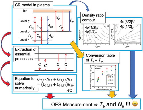
This paper describes the use of Optical Emission Spectroscopy (OES) to measure electron densities and temperatures in non-equilibrium plasmas. The ways to interpret relative line-intensities of neutral argon atoms are evaluated based upon a collisional-radiative model including atomic collisional processes. A conversion from an excitation temperature determined from relative line intensities assuming a Boltzmann population distribution to the thermal electron temperature in the electron temperature range 1–4 eV and electron density range 10¹⁰–10¹² cm^–3 is given. Procedures to obtain electron temperature T_e and density N_e of non-equilibrium argon plasma by OES measurement with collisional radiative model.

Graphical Abstract

KEYWORDS:

• Non-equilibrium atmospheric-plasma
• Ar plasma
• optical emission spectroscopy (OES)
• electron temperature
• collisional radiative model

PACS:

• 52.70.Kz (Optical (ultraviolet
• visible
• infrared) measurements)
• 52.70.-m (Plasma diagnostic techniques and instrumentation)
• 52.25.Os (Emission of electromagnetic radiation)

1. Introduction

Reactive plasmas are generated stably and continuously when electric power is supplied to rarefied rare gas, typically argon, with some amount of reactive gases. These plasmas are, generally, in a state of non-equilibrium, and contain higher-density reactive species with high-energy performance than the values given in the chemical composition equilibrated with its gas temperature [1–4]. Of course, thermal plasmas are also useful to produce reactive species using its thermal equilibrium condition [5,6]. However, heat removal from the thermal plasma torch as well as large electric current supply is not very easy in terms of engineering. In many industrial applications, to avoid thermal damage not only to the product but also to the apparatus is a crucial issue to overcome. Chemical species desired should be produced even under low gas-temperature conditions, and in this respect, the non-equilibrium plasma provides one of the best engineering answers. These reactive species can be applied to many fields of practical industry, e.g. microelectronics, semiconductors, material engineering, etc., where low-pressure discharge plasmas have been utilized for a long time with practical levels of industry. For example, in the microelectronics engineering, dry etching processes have been widely applied for more than 30 years for the commercial fabrication of memories [7], where typically, fluorine radicals are generated from fluorocarbon gases in the argon-based low-temperature plasmas like CCP [8,9], ICP [10,11], ECR plasmas [12,13], or others, and applied to material etching out of the substrate. On the other hand, for thin-film deposition processes like photovoltaic-device manufacturing, silicon-based materials are quite often deposited on substrates from the SiH₄ or other silicon-compound gaseous molecules [14,15]. There are also many applications of the plasma processes for graphene-like carbon material preparation [16,17]. Raw material molecules are dissociated into radicals in the non-equilibrium plasmas, which will be deposited on the appropriate substrate in the plasma chamber to form thin-film electronic devices.

Apart from electronical engineering, many materials are industrially processed with non-equilibrium plasmas. An example is a surface modification process of metals (SUS or Ti) with nitrogen radicals with nitrogen plasma, where the surface nitride or atomic nitrogen diffusion layer strongly hardens the surface, which offers practical hardness and durability of many metallic tools such as cutting edge of drills or lathes, cylinders of automobile engine, or even turbine blades [18,19].

In addition, recent technical progress makes it possible to generate the non-equilibrium plasmas under atmospheric-pressure discharge condition, most of which can be touched safely. Of course, these discharge plasmas can be generated also in liquid phase, and the number of applied fields is increasing, such as medical, agricultural, food and textile industries [20–26]. When these plasmas are applied to practical engineering, fundamental plasma parameters must be observed to control production quality and process conditions [27,28]. Particularly, the electron temperature and density must be measured, since they take a main role to generate reactive species in the state of non-equilibrium and determine the process rate [29,30]. However, the standard methods of parameter measurement have not been established yet, especially for the electron temperature measurement. Although the electrostatic probes are the most basic measurement tool for the low-pressure discharge plasmas, they are basically difficult to apply measure the plasma parameters of atmospheric-pressure discharge. This is because the assumption of collisionless sheath, as a prerequisite condition for the probe analysis, does not hold in the atmospheric-pressure plasmas due to a short mean free path of electrons. Hence, theoretical analysis of the probe data under atmospheric-pressure condition becomes too complicated to apply for practical measurement [31,32]. Before that, the size of the atmospheric-pressure plasmas is generally very small, and consequently, it is sometimes difficult to insert the probe-electrode. It should be also noted to apply the probe voltage should essentially disturb the discharge condition, which is completely undesirable for the plasma measurement.

Meanwhile, in the optical emission spectroscopy (OES) measurement of plasmas, optical radiations emitted from the plasma are guided into spectrometric system, followed by detection with opto-electric receivers, which means that the plasma is not perturbed with the measurement. In this respect, the OES measurement is quite a desirable measurement method of plasmas. If the plasma is in the state of local thermodynamic equilibrium (LTE), the observed line intensities give the number densities of the excited states, which directly shows the temperature as the slope of the Boltzmann plot, because they obey the Boltzmann distribution. However, when the radiation emission is from the plasmas in the state of non-equilibrium, the excited-state number densities corresponding to the line intensities cannot be described with the Boltzmann distribution [33–38]. Therefore, to obtain the information about the plasma from the OES measurement, the excitation kinetics in the plasma must be understood well in terms of atomic and molecular processes in the plasma itself. Particularly, the excited-state densities should be mathematically formulated with the plasma parameters, such as the electron temperature and density, which is common both to low-pressure and to atmospheric-pressure discharge plasmas, provided that the plasma is in the state of non-equilibrium. Even if the plasma is in such a state, when the excitation kinetics is formulated correctly based on the elementary atomic processes, the plasma parameters are well associated with the excited-states populations [39].

Concerning classifications of the optical emission from plasmas, line and continuum spectra are observed. In this review, the former one is concentrated on, since the line spectra are the easier of the two to analyze the plasma parameters, where each line intensity indicate the number density of the upper state of the corresponding transition for its wavelength. When the relationship between the excited-state populations and the plasma parameters is described, an excitation kinetic model is frequently applied, which is referred to as the ‘Collisional Radiative model’ (CR model) and will be detailed in the next section [33–38]. Owing to economical and historical backgrounds, argon is usually chosen as a mother discharge gas species in most of the plasma processes, and consequently, the argon CR model becomes necessary where the excitation kinetics of argon is well modeled in terms of rate equations to describe time evolutions of number densities of excited states [40–45]. In this application, the input and the output of the CR model become reversal. Namely, when the electron temperature and density are determined from the CR model, the methodology to apply the CR model must be physically developed from the number densities of the excited states that must be observed easily in the OES measurement, which become input parameters of this application. This discussion is given in the next section.

It should be stated here that many excellent papers have been already published where the argon CR model is applied to measure the plasma parameters in the low-temperature non-equilibrium plasmas, particularly, for the recent years. The relationship between the excitation temperature and the electron density, whose principle is later explained in section 3.3, was also widely investigated, for example, by Park and Choe [46]. For the optical thick conditions, Zhu and his co-workers published a remarkable theory that explained experiments [47]. If the CR model is coupled with the OES experiments, even the number densities of metastable levels can be determined, which have been demonstrated [48]. The discrepancy of the electron energy distribution function (EEDF) from the Maxwellian has been also discussed with the CR model for the argon plasmas [49]. Even for the arc-discharge conditions, validity of the LTE condition is being examined in terms of the excitation population kinetics with the Ar-CR model [50]. Recently, the OES line-intensity measurement assisted with the CR model is being applied to understand the electron temperature of atmospheric-pressure discharge argon-based plasmas for various applications of material applications [51–55], energy applications [56–58], or aeronautical applications [59]. Of course, many reports are published relevant to the electron temperature measurement of argon-based low-pressure discharge plasmas by the OES measurement assisted with the CR model [60]. Simplification of the Ar CR model is also discussed in terms of statistical mathematics like principal component analysis [61,62].

On the other hand, when the OES measurement is carried out for the observation of atmospheric-pressure discharge plasmas, it has been reported that their continuum radiation has sufficient intensity for the detection of general spectrometric systems, which is rather difficult for the low-pressure discharge plasmas because of the low intensity. The advantage of the continuum radiation is being reported for the atmospheric-pressure plasmas [30]. However, this should be discussed in a different article in the future, since the physics to interpret the radiation data is completely different.

2. Overview of the CR model

2.1. Formulation

For simplicity, all the ions in the plasma are assumed to be singly charged ones, and the discharge plasma of a pure monatomic gas species (e.g. argon, helium, or other rare gas species) is considered. When the excitation kinetics of a certain electronically excited atomic state p, the p-th excited state counted from the ground state (now the ground state is defined as p = 1), are considered in the plasma, generally, the time evolution of its number density N_p can be sufficiently described only with the following elementary processes, i.e. (i) excitation and deexcitation by electron collisions with an atom in the level q₁ (q₁ ≠ p), (ii) population by radiative decay from the higher level q₂ (q₂ > p) and depopulation to the lower level q₃ (q₃ < p), (iii) ionization loss from the level p by electron collisions and its reversal process, three-body recombination, to the level p, and (iv) radiative recombination to the level p. In short, the population and depopulation of the level p are described with the electron collision processes, (i) and (iii), and with the radiative processes, (ii) and (iv). In this respect, this excitation kinetic model is referred to as the Collisional-Radiative (CR) model [33–43]. Figure 1 schematically illustrates the population/depopulation kinetics described with the CR model.

Figure 1. Schematic diagram of excitation kinetics of the level p in the collisional-radiative (CR) model. Red arrows indicate electron collisional processes, while the blue arrows indicate radiative processes. Characters in the figure correspond to their rate coefficients in Equation (1).

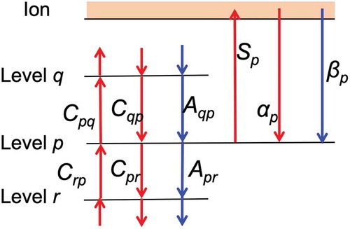
Of course, when the discharge condition becomes specified like the atmospheric-pressure discharge, some modification to the CR model becomes necessary. For the atmospheric-pressure plasmas, atomic collisions, i.e. so-called ‘quenching processes’, must be included in the excitation kinetic processes [40–45]. Hereafter, to make the CR model possible to treat the atmospheric-pressure discharge, the collisional excitation and deexcitation with the ground-state atom are included into the present CR model. Then, the following rate equations are obtained for the time evolution of the population density N_p of the level p (p ≥ 2) with the assumption that the ground-state density N₁ is constant:

(1) $\begin{array}{rl}& \frac{\mathrm{d}{N}_p}{\mathrm{d}t}=\sum _{q\ne p}{C}_{qp}{N}_q{N}_{\mathrm{e}}+\sum _{q\ne p}{K}_{qp}{N}_q{N}_1+\sum _{q>p}{\mathrm{\Lambda }}_{qp}{A}_{qp}{N}_q+\left({\alpha }_p{N}_e+{\beta }_p\right)N_{\mathrm{e}}{N}_{\mathrm{i}}\\ & -\left[N_{\mathrm{e}}\left(\sum _{q\ne p}{C}_{pq}+S_p\right)+N_1\sum _{q\ne p}{K}_{pq}+\sum _{q<p}{\mathrm{\Lambda }}_{pq}{A}_{pq}\right]N_p,\end{array}$(1)

where C_qp is the rate coefficient of electron collisional excitation (q < p) or deexcitation (q > p) from level q to p, K_qp is that of the collisional excitation or deexcitation with the ground-state atom, A_qp is the transition probability from level q to p, Λ_qp is the optical escape factor for the transition. When the photo-absorption is negligible, such plasma or transition is referred to as ‘to be optically thin’. For processing plasmas in a lab scale setup, it is usually approximated that Λ_qp ~ 1 for p ≠ 1, that is, the plasma can be considered to be optically thin for the transitions to the excited state (not to the ground state). S_p is the rate coefficient of electron impact ionization of the level p, α_p is that of its reversal process, three-body recombination to the level p, β_p is that of photo-recombination to the level p, N_e is the electron density and N_i is the ion density. The details of these atomic data or rate coefficients are specified elsewhere [40,44,45]. The transition probabilities are constants. Other rate coefficients can be calculated with the corresponding cross sections σ(ϵ) as a function of the electron energy ϵ and the electron energy distribution function F(ϵ). For example, that of the electron collision excitation is described as follows [39–45]:

(2) $C_{pq}=\sqrt{\frac{2}{m_{\mathrm{e}}}}\underset{{\in }_{\mathrm{t}\mathrm{h}}}{\overset{\mathrm{\infty }}{\int }}\sqrt{\in }\sigma \left(\in \right)F\left(\in \right)\mathrm{d}\in ,$(2)

where ϵ_th is the threshold energy of the excitation process and m_e is the electron mass. Even when the EEDF is not Maxwellian, which is usually the case with low-pressure discharge plasmas for electronic engineering or material processing, Equations (1) and (2) hold exactly. On the other hand, the EEDF must be approximated with some functions when the observed line intensities are interpreted based on the CR model. As a first step of the approximation, the assumption of the Maxwellian EEDF is quite significant to determine the ‘electron temperature’ as the approximate one to control the plasma processing even though the ‘electron temperature’ should be understood as a kind of the ‘effective temperature’.

Since diffusion loss or three-body collisions with neutral particles are negligible processes for the levels except for metastables, the time derivative, or the left-hand side, of Equation (1) can be approximated to be zero, which is referred to as the quasi-stationary approximation, which has been confirmed to be justifiable generally [33–40,44,45,63,64]. For this occasion, Equation (1) becomes linear for the unknown quantity N_p (p ≥ 2), and consequently, its analytic solution can be obtained. When the values of N₁ and N_e (= N_i) are already known, N_p can be described as a summation of two components as follows:

(3) $N_p=Z_p{r}_0\left(p\right)N_{\mathrm{e}}{N}_{\mathrm{i}}+\frac{Z_p}{Z_1}{r}_1\left(p\right)N_1=n_0\left(p\right)+n_1\left(p\right),$(3)

with

(4) $Z_p=\frac{g\left(p\right)}{2g_{\mathrm{i}}}{\left(\frac{h^2}{2\pi m_{\mathrm{e}}k{T}_{\mathrm{e}}}\right)}^{3/2}\mathrm{e}\mathrm{x}\mathrm{p}\left[\frac{\chi \left(p\right)}{k{T}_{\mathrm{e}}}\right],$(4)

where r₀ and r₁ denote the population coefficients, which can be expressed with the rate coefficients and N_e, g(p) is the statistical weight of the level p, g_i is that of the ion, h is the Planck constant, χ(p) is the ionization potential of the level p, and k is the Boltzmann constant. Equation (3), as a solution to Equation (1), consists of two terms, where the first term n₀(p) is in proportion to the product N_eN_i, while the second term n₁(p) is proportional to the ground-state density N₁. The terms n₀(p) and n₁(p) are referred to as ‘the recombining plasma component’ and ‘the ionizing plasma component’, respectively [33–40,63].

2.2. Dependence of essential population and depopulation mechanisms on various plasma parameters

Most of the processing plasmas are categorized as ‘ionizing plasmas’, where the neutral particles are ionized volumetrically, and the recombination takes place on the inner surface of the discharge tube or chamber wall, except for the remote plasmas that are applied after transportation from the discharge region. For low-pressure discharge ionizing plasmas to which atomic collisional processes are negligible, i.e. K_qp ~ K_pq ~ 0, the dependence of n₁ on the level number p has been examined in detail up to the present time [33–39]. For hydrogen-like ions, the dependence of N(p)/g(p) on p is summarized in Figure 2 for the level number p and for the reduced electron density N_e/z⁷, where z is the nuclear charge of the hydrogen-like ion [33–38,63]. The lines in Figure 2 marked as ‘Griem’ and ‘Byron’ indicate the Griem’s boundary p_G and the Byron’s boundary p_B, respectively, each of which is given as follows:

(5) $p_{\mathrm{G}}\cong 95{\left(N_e\left[\mathrm{c}{\mathrm{m}}^{-3}\right]/z^7\right)}^{-2/17},$(5)

(6) $p_{\mathrm{B}}\cong {\left(z^{2}R/3k{T}_{\mathrm{e}}\right)}^{1/2},$(6)

Figure 2. Schematic diagram of the ‘phases’ of the hydrogen-like ionizing plasma; i.e. ‘Corona phase’, ‘Saturation (Thermodynamically Equilibrium: TE) phase’ and ‘Saturation (Ladder-like) phase’. p is the principal quantum number, N/g is the reduced population density. The straight arrow indicates electron collision excitation/deexcitation process, while the wavy arrow indicates radiative process. Horizontal axis denotes the logarithm of reduced electron density divided by z ⁷. The phase transition lines ‘GRIEM’ and ‘BYRON’ indicate the Griem’s boundary (Equation (5)) and the Byron’s boundary (Equation (6)), respectively [33,37].

where R is the Rydberg constant. When the atoms or ions are not hydrogen-like, the following ‘effective principal quantum number’, p*, leads to the same discussion for the population distribution N_p [64]:

(7) $p^{\ast }=z{\left[R/\chi \left(p\right)\right]}^{1/2}.$(7)

When Figure 2 is applied to processing plasmas, the area marked with ‘Saturation (TE)’ is difficult to find because the Byron’s boundary becomes too small. Therefore, the region designated as ‘Corona’ region in Figure 2 has been frequently applied for the diagnostics of electron temperature. Here in the corona region, the excited states are mainly populated with the electron collisional excitation from the ground state, whereas they are depopulated with radiative transition, which is referred to as ‘Corona equilibrium’ [33–42]. The corona phase is situated lower than the levels given by the Griem’s boundary level p_G. However, when the electron density becomes higher, the Griem’s boundary becomes lower as is shown in Equation (5), and consequently, the corona equilibrium does not hold for the levels observed practically. This makes it difficult to determine the electron temperature. In the meantime, for the atmospheric-pressure discharge plasmas, atomic collisional processes, or quenching processes, become dominant in the excitation kinetics.

Nevertheless, in the above discussion from Equation (5) through Figure 2, the atomic collisions have not been included at all. Hence, the excitation kinetics should be reconsidered for each discharge condition, some of which includes cumulative excitation or atomic-collisional quenching processes. This kind of improvement of excitation kinetic models has been developed for these 20 years, mainly for low-pressure discharge plasmas with trace rare gas OES (TRG-OES) [65–67], or simple modification of the corona model [68–70].

However, each improvement in many research works has been, in some sense, specialized for the corresponding experimental discharge condition, and not generalized. For example, if the corona model does not hold and the cumulative excitation is dominant for rather high-electron density plasmas, the modified Boltzmann plot method (which will be later explained in the beginning of section 3.3) does not work. Thus, the industrial plasma users desire some systematic model of excitation kinetics in discharge plasmas, which is suitable to determine the electron temperature and density from the OES observation, to apply the kinetic model to their plasmas developed for semiconductors or material processing, even if the model is rough and abstract. The objective of this paper is to describe further general methods to analyze excited-state populations in arbitrarily non-equilibrium plasmas measured with the OES observation assisted with the CR model. Therefore, in the following sections, some of the methodology will be described to interpret the OES data to determine the electron temperature and density of argon plasma, practically with the argon CR model.

3. Applications of the argon CR model

3.1. Extraction of dominant elementary processes

The OES measurement directly gives the number densities of the excited states. Therefore, when the electron temperature and density are determined with these data, the CR model is applied in the opposite direction as a so-called inverse problem. Of course, the direct fitting for the observed OES data with T_e and N_e can be possible. However, the agreement of the parameters or the applicability depends strongly upon each discharge condition, and consequently, the applicable range must also be considered [71].

The basic strategy in the present study is as follows. That is, the governing equations as Equation (1) = 0, which describes the population balance of each level with elementary processes on the excitation kinetics, i.e. the rate equations, must be simultaneously solved for the number of unknown quantities. Then, by substituting the number densities N_p observed by the OES measurement into the rate equations, they are solved for the electron temperature T_e and density N_e [45,72,73].

In order to realize such an OES measurement, following two conditions must be satisfied in the modeling of the excitation kinetics [74]:

1. In the kinetic equations, the model must not include the level densities that cannot be observed by the OES measurement. Otherwise, they must be able to be calculated from other level densities self-consistently in the model.

2. The model must be a simplified one by extracting ‘dominant’ processes that characterize the excitation kinetics with a large proportion in the population/depopulation rate.

For example, when the right-hand-side (RHS) of Equation (1) is set to be equal to zero, of course, the equation becomes exact. However, if such an equation is applied to a real determination of the electron temperature, all the excited states are to be included in the simultaneous equations, which forces that the density of all the excited states must be measured. This makes the equations quite far from practical use. Therefore, the basic strategy becomes as follows. Some dominant positive terms of RHS in Equation (1) in the population flow to the level p are to be picked-up in the descending order until the summation of the terms becomes about 80% (or lower, if difficult) of the total inflow to the level p, over the electron temperature and density expected to the objective plasmas. Likewise, the dominant negative terms of RHS in Equation (1) in the depopulation flow from the level p are also to be picked-up until their summation becomes about 80% of the total outgoing flow. These procedures are referred to as ‘extraction of dominant terms’. Namely, the total population terms E_POP(p) and depopulation terms E_DEP(p) to and from the level p are exactly formulated as follows, respectively:

(8) $E_{\mathrm{P}\mathrm{O}\mathrm{P}}\left(p\right)=\sum _{q\ne p}{C}_{qp}{N}_q{N}_{\mathrm{e}}+\sum _{q\ne p}{K}_{qp}{N}_q{N}_1+\sum _{q>p}{\mathrm{\Lambda }}_{qp}{A}_{qp}{N}_q+\left({\alpha }_p{N}_{\mathrm{e}}+{\beta }_p\right)N_{\mathrm{e}}{N}_{\mathrm{i}}$(8)

and

(9) $E_{\mathrm{D}\mathrm{E}\mathrm{P}}\left(p\right)=\left[N_{\mathrm{e}}\left(\sum _{q\ne p}{C}_{pq}+S_p\right)+N_1\sum _{q\ne p}{K}_{pq}+\sum _{q<p}{\mathrm{\Lambda }}_{pq}{A}_{pq}\right]N_p.$(9)

At this moment, with a kind of threshold value Θ, effective approximated values of E_POP and E_DEP are defined as E_POP* and E_DEP* as follows, respectively:

(10) $E_{\mathrm{P}\mathrm{O}\mathrm{P}}^{\ast }\left(p\right)=\mathrm{\Theta }{E}_{\mathrm{P}\mathrm{O}\mathrm{P}}\left(p\right),E_{\mathrm{D}\mathrm{E}\mathrm{P}}^{\ast }\left(p\right)=\mathrm{\Theta }{E}_{\mathrm{D}\mathrm{E}\mathrm{P}}\left(p\right).$(10)

Based on these approximations, dominant terms are to be extracted from the RHS of Equations (8) – (9) [39,72–74]. If the above model is made to cover a wide range of the electron temperature and density, too many parameters must be extracted from the summation of the RHS of these equations. Consequently, the model includes too many levels to be measured, which is not practical at all. In the meantime, when strictness is given priority, the parameter Θ becomes too large to incorporate the elementary processes, which deteriorates practicality of the model. Therefore, after due consideration on the measurement purpose and the characteristics of the object, the practical model of the excitation kinetics must be constructed under the assumption of the appropriate range of electron temperature and density as well as the threshold value Θ [72–74].

Hereafter, an example of this scheme is introduced, which was developed for the purpose of measurement of the electron temperature and density of DC hollow cathode argon plasma [72]. Prior to the OES measurement, Langmuir probe measurement had shown the possible range of the electron temperature and density as 0.8 ≤ T_e [eV] ≤ 2.0 and 10¹⁴ ≤ N_e [cm^–3] ≤ 10¹⁵, respectively [75]. After the comparison among various excited states on the excitation kinetics, the level p = 20 (4d + 6s) is chosen for the electron temperature measurement, because most of the counterparts of the dominant population/depopulation to/from p = 20 can be spectroscopically observable. Figure 3 schematically shows the excitation kinetics of the level 20. Its excitation kinetics can be separated into two cases according to the electron temperature, i.e. low-temperature case (a) 0.8 ≤ T_e [eV] ≤ 1.2, and high-temperature case (b) 1.2 ≤ T_e [eV] ≤ 2.0. For both cases, the population balance equation is obtained to the level 20 with the threshold value Θ ≥ 90%. For case (a), the following relations are found:

(11) $C_{25,20}{N}_{25}+C_{27,20}{N}_{27}+C_{23,20}{N}_{23}=\left(C_{20,23}+C_{20,25}+C_{20,27}\right)N_{20}$(11)

Figure 3. Essential elementary processes for the population and depopulation of the level N = 20 (4d + 6s) for the electron temperature range (a) 0.8 ≤ T_e [eV] ≤ 1.2 and (b) 1.2 ≤ T_e [eV] ≤ 2.0. The symbol C denotes the electron collision process. It is found that C_23,30N₂₃$\simeq$C_20,23N₂₀ under the condition (a), and consequently, the equation to be solved can be simplified.

and

(12) $C_{23,20}{N}_{23}\cong C_{20,23}{N}_{20}.$(12)

Consequently, it is found that the equation

(13) $C_{25,20}{N}_{25}+C_{27,20}{N}_{27}=\left(C_{20,25}+C_{20,27}\right)N_{20}$(13)

should be solved for the case (a). On the other hand, for case (b), the population balance of the level 20 becomes

(14) $C_{18,20}{N}_{18}\cong C_{20,23}{N}_{20}.$(14)

Then, it follows that the number densities to be observed are those of the levels 18 (5p), 20 (4d + 6s), 25 (6p), and 27 (5d + 7s). Figure 4 shows the results of the proposed OES measurement together with those with the Langmuir probe plotted against the discharge pressure [72]. The agreement between both results is considered to be sufficient for practical use of the OES method. It should be noted that the electron temperature can be obtained with sufficient accuracy for Equation (14) that is typical excitation kinetics as ladder-like excitation. This process had been considered to be impossible for T_e determination of hydrogen-like plasma [33–38] due to the cancellation of T_e-dependence of the rate coefficient C. However, it was found that this was not the case for the argon plasma with more accurate description of the rate coefficients.

Figure 4. Comparison of the electron temperature measured with the Langmuir probe and that with the OES method assisted with the CR model described by Equations (11) – (14) as schematically shown in Figure 3 for the hollow cathode DC discharge argon plasma for its discharge current 6 A [72].

It was very difficult to determine the electron density with the same procedure. This is partly because of the cancellation of the term N_e in the population balance equation unless the rate of radiative processes has the same order with that of electron collision processes. Further details are given in [72].

The scheme of the ‘Extraction of dominant elementary processes’, explained in this section, is practical and useful, particularly for low-electron density plasmas (because of the availability to the determination of the electron density), which is not limited to the discharge condition described above. The reference [72] has been sometimes cited even recently, despite the passage of 18 years since its publication. Consequently, it is considered to be put to practical use still now. This scheme is now being expanded to the microwave discharge argon plasma with its discharge pressure several Torr [74]. A novel model with the lower threshold value Θ is also being developed for the purpose of enlargement of applicable range of the plasma parameters [72–74].

3.2. Two-line-pair method

Considerable simplification is adopted in the scheme described in 3.1 in order to apply the CR model to the practical OES measurement. However, some users claim that the scheme for OES measurement described in section 3.1 is still complicated, and complain its hard applicability. It is worthwhile to discuss the possibility to apply the density ratio of two excited states for the simple OES monitoring of the electron temperature and density.

In this section, the discussion is focused on the low-pressure discharge argon plasma. Parameter survey is carried out for the density ratio of excited states under the following discharge condition: the plasma diameter D = 20 mm, the gas temperature T_g = 500 K, and the discharge pressure P = 7 mTorr, over the parameter range 2 ≤ T_e [eV] ≤ 8 and 10¹⁰ ≤ N_e [cm^–3] ≤ 10¹³. As a result, some level-pairs are found to be strongly dependent on either one of the plasma parameters, T_e or N_e [76,77], an example of which is shown in Figure 5 as a contour of density ratio. Even if the ratio depends on both parameters, provided that two level-pairs with opposite dependences are found, T_e and N_e can be determined as an intersection of two curves in the density ratio contours.

Figure 5. Density contour of number density ratio of the excited states calculated with the argon CR model, displayed on T_e-N_e map. (a) 4p’ [1/2]₀/4p[1/2]₀, and (b) 4d[3/2]°/4p[1/2]₀ [44].

For example, the level pair (4p’ [1/2]₀) and (4p[1/2]₀), as the line intensity ratio of 750.4 nm and 751.5 nm, does not strongly dependent on N_e for the electron temperature range 3 ≤ T_e [eV] ≤ 5, as shown in Figure 5(a), whereas that of (4d[3/2]°) and (4p[1/2]₀) in Figure 5(b), as the intensity ratio of 675.3 nm and 751.5 nm, shows the opposite dependence over the density range N_e ≤ 10¹¹ cm^–3. Thus, in principle, if two density-pairs are found to have different dependences on the set of T_e and N_e, i.e. the density contour lines do not show parallel traces, they can determine the parameters T_e and N_e as an intersection of the contour lines of the density ratio of level-pairs [76,77]. This scheme applies only two line-pairs to determine the parameters, and consequently, statistical improvement with many line intensities cannot be expected for precision. The accuracy of the plasma parameters of this method depends strongly upon the quality of the cross sections or rate coefficients in the CR model. Therefore, the atomic data like cross sections should be updated frequently. Various schemes for the determination of T_e and N_e with the OES data have been proposed with this methodology, one of which is shown in Figure 6 [76,77]. Similar research reports have been published [78–80].

Figure 6. Electron temperature and density measured for the argon plasma generated in the small helicon device (SHD) developed for the electric propulsion of satellite maneuver [81–83]. Red open squares are those measured with the scheme described in section 3.2, with two intensity ratios of (687.1 nm)/(763.5 nm) [= 4d[1/2]°/4p[3/2] = 4d₅/2p₆] and (549.6 nm)/(751.5 nm) [= 6d[7/2]°/4p[1/2]₀ = 6d’₄/2p₅] with most revised cross section data in Ref [78]., while green open diamonds are the same but with the old cross section data in Ref [40]. Blue filled dots are those measured with a Langmuir single probe.

The above discussion is addressed to low-pressure discharge plasmas. Of course, it can be extended to higher-pressure discharge plasmas. In that case, however, the collision processes with the ground-state atoms or molecules become dominant in the excitation kinetics, and consequently, the gas temperature T_g should be included into the determination process of the electron temperature and density [45]. Therefore, practically, the gas temperature should be obtained as an approximate value, with the OES measurement of rotation temperature of diatomic molecules with band spectra, and followed by the scheme described in the above paragraphs.

3.3. Conversion table method from the excitation temperature

If we understand that the plasma to be observed is in the Corona equilibrium, or in the ‘Corona’-phase region in Figure 2, a more graphical method to obtain the electron temperature is already proposed with a modified Boltzmann plot [84]. Gordillo-Vázquez et al. proposed the following equation to fit the OES population data with the electron temperature T_e for the excited-level populations in the corona phase:

(15) $ln\left(\frac{I_{ij}{\sum }_{i>j}{A}_{ij}}{h{\nu }_{ij}{A}_{ij}{b}_{1j}}\right)=-\frac{E_i}{k{T}_{\mathrm{e}}}+\mathrm{C}\mathrm{o}\mathrm{n}\mathrm{s}\mathrm{t}.,$(15)

where I_ij and ν_ij are the line intensity and the frequency of the transition from i to j state, respectively, E_i is the excitation energy of the level i, and b_1j is a parameter of the level j determined with the energy E_j and electron collisional cross section (or rate coefficient) from level 1 to j. After the proposal of this data fitting procedure, several papers reported that the electron temperature determined with the OES measurement was improved in its accuracy [85,86].

However, as was stated at the end of Section 2.2, if the corona model does not hold and the cumulative excitation is dominant for rather high-electron density plasmas, the modified Boltzmann plot method, or Equation (15), cannot be applied to the real OES analysis. More common method to non-equilibrium plasmas should be searched for.

Hereafter, the discussion is limited to the electron temperature of atmospheric-pressure non-equilibrium argon plasmas. In the previous subsection, the basis of the OES measurement is the number densities of two excited-levels to determine the plasma parameters, because they are determined with the excitation kinetics in the plasma. However, even for the OES measurement of the plasma in a state of LTE, it should be pointed out as too rough to determine the temperature by the densities of only two levels. Generally, when the electron temperature is determined from the OES measurement for the LTE plasma, the Boltzmann plot is drawn, where the slope of straight line is found to be the excitation temperature. In this procedure, the straight line is determined by the least square method from many observed plots to show the relationship between the logarithm of the reduced number densities ln(N_p/g_p) and the excitation energy of the corresponding levels E_p. However, when the object to be measured is in the state of non-LTE, the Boltzmann plot generally cannot make a straight line. Consequently, even if many observed data are added to the Boltzmann plot, it is difficult to improve the accuracy of the temperature.

To overcome the difficulty described above, the following procedure is proposed by applying the excitation temperature T ^ex. Even if the plasma is in the state of non-LTE, the excitation temperature T ^ex can be defined as the slope of the straight line determined by the least square method with the Boltzmann plot. The accuracy of T ^ex can be improved statistically with adding many observed OES data to the Boltzmann plot. For the argon CR model, several levels with the same quantum numbers are treated in a lump, therefore, many states can be added. For example, for in the CR model, the ‘5p’ level is prepared as a representative of 5p[1/2], 5p[3/2] and 5p[5/2]. On the other hand, when the electron density N_e and the gas temperature T_g are fixed, the CR model calculation gives the relationship between the electron temperature T_e and the excitation temperature T ^ex determined for some levels to be noticed. When this procedure is repeated for the expected electron temperature range, the conversion table can be obtained between the electron temperature T_e and the excitation temperature T ^ex. After the preparation of this conversion table, T ^ex should be determined by the OES measurement with many line intensities with considerable accuracy, and the table gives the corresponding electron temperature [45,87,88]. Of course, the applicability of this procedure is limited to the parameter range where the excitation temperature is less dependent on the electron density N_e or the gas temperature T_g. Nevertheless, this procedure is practically convenient to use and meaningful as a simple real-time monitoring at the engineering site.

When the argon plasma is monitored with this scheme, the excitation temperature determined with 4p (plus 4p’) group and the 5p (plus 5p’) group is appropriate for the monitoring because of a large energy difference, at least 1 eV [89,90]. Figure 7 shows the Boltzmann plot as a principle to determine the excitation temperature T ^ex_5p-4p for 5p-4p levels with the electron density N_e = 10¹¹ cm^–3 and T_g = 1000 K. It is understood that T ^ex_5p-4p monotonically increases as T_e increases. Of course, this kind of plots can be drawn for other electron density and gas temperature. Figure 8 shows the relationship between T_e and T ^ex_5p-4p for the electron density range 10¹⁰ ≤ N_e [cm^–3] ≤ 10¹². The electron temperature can be determined on the basis of this figure with the excitation temperature determined with many levels of 5p groups and 4p groups. As was mentioned before, both 4p and 5p groups have many sublevels, hence, the accuracy of the excitation temperature can be improved statistically with line-intensity measurement for many levels. This scheme was applied to a microwave discharge atmospheric-pressure argon plasma (microwave power 100 W, Ar flow rate 8 L/min [91–93]), which indicated that T_e of this plasma is about 0.8–0.9 eV. It is confirmed that this scheme gives almost the same electron temperature with that deduced from the continuum emission measurement for several kinds of atmospheric-pressure non-equilibrium plasmas with low electron temperature, which is considered to be a justification of the ‘conversion table method from the excitation temperature’ proposed here [45,87,88].

Figure 7. Reduced number densities N/g of the levels 4p, 4p’, 5p and 5p’, calculated with the argon CR model normalized by that of the 4p[1/2]₁ level. Linear fitting in the figure gives the excitation temperature with its slope. When the fitting is conducted, the statistical weight is reflected for the regression calculation.

Figure 8. The relationship between the electron temperature T_e and the excitation temperature T^ex determined for 4p – 5p levels calculated with the argon CR model. It is assumed that the gas temperature T_g = 1500 K and the discharge tube radius R = 5 mm, with the electron density N_e = 10¹⁰–10¹² cm^–3 [87,88].

4. Conclusion

The findings at the present time have been stated on the OES measurement of non-equilibrium argon discharge plasma, as an application of the CR model, particularly for the determination of the electron temperature and density from the number densities in non-LTE state. First, the CR model was explained in terms of excitation kinetics in the plasmas, which describes the excited-state number densities of any non-LTE state as functions of the electron temperature, density and the ground-state neutral atom. Then, three methods were described to interpret the OES data of argon discharge plasmas based on the Ar-CR model through the atomic processes in the plasmas: (1) extraction of dominant elementary processes, (2) two-line-pair method, and (3) conversion table method from the excitation temperature, where the electron temperature ranges from 1 eV to 4 eV and electron density ranges from 10¹⁰ cm^–3 to 10¹² cm^–3, which should be more practical range for industrial applications.

In the first method ‘extraction of dominant elementary processes’, essential elementary processes of the population/depopulation rates of some appropriate excited levels should be extracted to describe the population balances of the level with the CR model. These balance equations will give a set of non-linear equations to deduce the electron temperature and density, where many excited-level densities appear as unknown parameters to be observed with the OES measurement. This method is versatile, sensitive to the excited-level density variation, and gives the values of T_e and N_e that agree with the probe analysis. However, to construct the kinetic model is a troublesome task that requires a long time. It should be also pointed out that the excitation kinetic model must be modified according to the expected T_e-N_e range.

On the other hand, the second method, ‘two-line-pair method’, is based on the application of two contour diagrams on the T_e-N_e maps with respect to the density-ratio of some appropriate excited-state number densities. These contour maps should be prepared with the CR-model calculation prior to the experimental OES observation. When four line-intensities are measured and two values of their line-intensity ratios are calculated, the intersection of the two contour lines will indicate the values of the electron temperature and density. This method is simple and convenient. However, the results are quite sensitive to the cross sections and the transition probabilities applied in the CR model, and consequently, the atomic data in this model must be updated as much as possible.

Finally, the third method ‘conversion table method from the excitation temperature to the electron temperature’ is introduced for the experimental improvement of the accuracy of the observed electron temperature. The CR-model gives the excitation temperature between some appropriate level pairs as functions of the electron temperature, density, the ground-state density and the gas temperature. When more line-intensities are observed with the OES measurement, the accuracy of the resultant excitation temperature given by the slope of the Boltzmann plot can be improved statistically. Then, when the conversion table from the excitation temperature to the electron temperature is well established with the CR model calculation prior to the experiments, the accuracy of the electron temperature is also improved with numbers of lines observed. However, this method is valid only when the excitation temperature is almost independent of the electron density or of the neutral density.

According to the requirement for the accuracy or practicality, the best method should be chosen for its feasibility. To confirm the validity of the electron temperature and density measured with one of the present methods, cross-checks should be conducted by other experimental methods based on different physical principles, e.g. laser scattering or line-width analysis, which should be continued hereafter.

Acknowledgments

Many of the achievements summarized here are based on the students’ effort of the past in the author’s laboratory of Tokyo Institute of Technology, Tokyo, Japan. The author thanks Dr K. Kano, Mr R. Kashiwazaki, Mr J. Mizuochi, Mr K. Ando, Mr Y. Yamashita, Mr H. Onishi, Mr F. Yamazaki, Mr Y. Hakozaki, and Mr R. Togashi. The author also thanks Dr M. Matsuzaki and Mr A. Nezu for their technical cooperation. Particularly, concerning Section 3.2, the author owes very much to Professor S. Shinohara of Tokyo University of Agriculture and Technology, and his co-workers.

Disclosure statement

No potential conflict of interest was reported by the author.

Additional information

Funding

This work was partially supported by JSPS KAKENHI Grant Numbers JP16540446, JP18540485 and JP26286070. Part of the results of this research is also due to academic cooperation with Canon Inc.

References

- Lieberman MA, Lichtenberg AJ. Principles of plasma discharges and materials processing. Hoboken, NJ: Wiley; 2005.
- Fridman A. Plasma Chemistry. Cambridge: Cambridge University Press; 2008.
- Hippler R, Kersten H, Schmidt M, et al. Low temperature plasmas. Weinheim, Germany: Wiley; 2008. vol. 257–281.
- d’Agostino R, Favia P, Kawai Y, et al. Advanced plasma technology. Weinheim, Germany: Wiley; 2008.
- Boulos MI, Fauchais P, Pfender E. Thermal Plasmas. New York, NY: Springer; 1994.
- Solonenko OP. Thermal plasma torches and technologies. Cambridge: Cambridge Int Science Publish; 2000.
- Nojiri K. Dry etching technology for semiconductors. New York, NY: Springer; 2015.
- Bia Z-H, Liu Y-X, Jiang W, et al. A brief review of dual-frequency capacitively coupled discharges. Current Appl Phys. 2011;11:s2.
- Ohtsu Y. Physics of high-density radio frequency capacitively coupled plasma with various electrodes and its applications. In: Plasma science and technology - basic fundamentals and modern applications. Ed. by Jelassi H. and Benredjem D., p. 209. Rijeka, Croatia: InTech Open Publishers; 2018. DOI:10.5772/intechopen.78387
- Lee H-C. Review of inductively coupled plasmas: nano-applications and bistable hysteresis physics. Appl Phys Rev. 2018;5:011108.
- Lei F, Li X-P, Liu Y-M, et al. Simulation of a large size inductively coupled plasma generator and comparison with experimental data. AIP Adv. 2018;8:015003.
- Geller R. Electron cyclotron resonance ion sources and ECR plasmas. London, UK: CRC Press; 1996.
- Tarey RD, Ganguli A, Sahu D, et al. Studies on plasma production in a large volume system using multiple compact ECR plasma sources. Plasma Sources Sci Technol. 2016;26:015009.
- Menéndez A, Sánchez P, Gómez D. Deposition of thin films: PECVD process. In: Silicon based thin film solar cells. Ed. by Murri R, Sharjah, UAE: Bentham Science; 2013. p. 29–57. DOI:10.2174/9781608055180113010006.
- Oehrlein GS, Hamaguchi S. Foundations of low-temperature plasma enhanced materials synthesis and etching. Plasma Sources Sci Technol. 2018;27:023001.
- Dato A. Graphene synthesized in atmospheric plasmas—A review. J Mater Res. 2019;34:214.
- Kim J-H, Sakakita H, Itagaki H. Low-temperature graphene growth by forced convection of plasma-excited radicals. Nano Lett. 2019. Article ASAP. DOI:10.1021/acs.nanolett.8b03769
- Kovala NN, Ryabchikov AI, Sivin DO, et al. Low-energy high-current plasma immersion implantation of nitrogen ions in plasma of non-self-sustained arc discharge with thermionic and hollow cathodes. Surf Coat Technol. 2018;340:152.
- Scheuer CJ, Zanetti FI, Cardoso RP, et al. Ultra-low—to high-temperature plasma-assisted nitriding: revisiting and going further on the martensitic stainless steel treatment. Mater Res Express. 2018;6:026529.
- Toyokuni S, Ikehara Y, Kikkawa F, et al. Plasma medical science. Cambridge, MA: Academic Press; 2018.
- Metelmann H-R, von Woedtke T, Weltmann K-D. Comprehensive clinical plasma medicine. New York, NY: Springer; 2018.
- Fridman A, Friedman G. Plasma Medicine. Chichester, UK: Wiley; 2013.
- Misra NN, Schlüter OK, Cullen PJ. Cold plasma in food and agriculture. London, UK: Elsevier; 2016.
- Yang Y, Cho YI, Fridman A. Plasma discharge in liquid: water treatment and applications. Boca Raton, FL: CRC Press; 2017.
- Shishoo R. Plasma Technologies for Textiles. Cambridge, UK: Elsevier; 2007.
- Nema SK, Jhala PB. Plasma technologies for textile and apparel. New Delhi, India: CRC Press; 2014.
- Ochkin VN. Spectroscopy of low temperature plasma. Weinheim, Germany: Wiley; 2009.
- Capitelli M, Celiberto R, Colonna G, et al. Fundamental aspects of plasma chemical physics – kinetics. New York, NY: Springer; 2016.
- Nikiforov AY, Leys C, Gonzalez MA, et al. Electron density measurement in atmospheric pressure plasma jets: stark broadening of hydrogenated and non-hydrogenated lines. Plasma Sources Sci Technol. 2015;24:034001.
- Park S, Choe W, Kim H, et al. Continuum emission-based electron diagnostics for atmospheric pressure plasmas and characteristics of nanosecond-pulsed argon plasma jets. Plasma Sources Sci Technol. 2015;24:034003.
- Xu KG, Doyle SJ, Measurement of atmospheric pressure microplasma jet with Langmuir probes. Vac J. Sci Technol A. 2016;34:051301.
- Trenchev G, Kolev S, Kissovski Z. Modeling a Langmuir probe in atmospheric pressure plasma at different EEDFs. Plasma Sources Sci Technol. 2017;26:055013.
- Fujimoto T. Plasma Spectroscopy. Oxford: Clarendon Press; 2004.
- Fujimoto T. Kinetics of ionization-recombination of a plasma and population density of excited ions. I. equilibrium plasma. J Phys Soc Jpn. 1979;47:265.
- Fujimoto T. Kinetics of ionization-recombination of a plasma and population density of excited ions. II. Ionizing plasma. J Phys Soc Jpn. 1979;47:273.
- Fujimoto T. Kinetics of ionization-recombination of a plasma and population density of excited ions. III. Recombining plasma–high-temperature case. J Phys Soc Jpn. 1980;49:1561.
- Fujimoto T. Kinetics of ionization-recombination of a plasma and population density of excited ions. IV. Recombining plasma–low-temperature case. J Phys Soc Jpn. 1980;49:1569.
- Fujimoto T. Kinetics of ionization-recombination of a plasma and population density of excited ions. V. Ionization-recombination and equilibrium plasma. J Phys Soc Jpn. 1985;54:2905.
- Kano K, Akatsuka H. Spectroscopic measurement of electron temperature and density in argon plasmas based on collisional-radiative model. Advances in plasma physics research. New York: NOVA Science Publishers. F. Gerard. 2002. Vol. 3. 55.
- Vlček J. A collisional-radiative model applicable to argon discharges over a wide range of conditions. I. Formulation and basic data. J Phys D Appl Phys. 1989;22:623.
- Vlček J, Pelikán V. A collisional-radiative model applicable to argon discharges over a wide range of conditions. II. Application to low-pressure, hollow-cathode arc and low-pressure glow discharges. J Phys D Appl Phys. 1989;22:632.
- Vlček J, Pelikán V. A collisional-radiative model applicable to argon discharges over a wide range of conditions. III. Application to atmospheric and subatmospheric pressure arcs. J Phys D Appl Phys. 1990;23:526.
- Vlček J, Pelikán V. A collisional-radiative model applicable to argon discharge over a wide range of conditions. IV. Application to inductively coupled plasmas. J Phys D Appl Phys. 1990;24:309.
- Bogaerts A, Gijbels R, Vlček J. Collisional-radiative model for an argon glow discharge. J Appl Phys. 1998;84:121.
- Akatsuka H. Excited level populations and excitation kinetics of nonequilibrium ionizing argon discharge plasma of atmospheric pressure. Phys Plasmas. 2009;16:043502.
- Park HY, Choe WH. Parametric study on excitation temperature and electron temperature in low pressure plasmas. Current Appl Phys. 2009;10:1456.
- Zhu XM, Tsankov TV, Luggenhölscher D, et al. 2D collisional-radiative model for non-uniform argon plasmas: with or without ‘escape factor’. J Phys D: Appl Phys. 2015;48:085201.
- Lee Y-K, Moon S-Y, Oh S-J, et al. Determination of metastable level densities in a low-pressure inductively coupled argon plasma by the line-ratio method of optical emission spectroscopy. J Phys D: Appl Phys. 2011;44:285203.
- Zhu XM, Pu YK. Determination of non-Maxwellian electron energy distributions in low-pressure plasmas by using the optical emission spectroscopy and a collisional-radiative model. Plasma Sources Sci Technol. 2011;13:267.
- Baeva M. A survey of chemical nonequilibrium in argon arc plasma. Plasma Chem Plasma Proc. 2017;37:513.
- Laurent M, Desjardins E, Meichelboeck M, et al. Characterization of argon dielectric barrier discharges applied to ethyl lactate plasma polymerization. J Phys D: Appl Phys. 2017;50:475205.
- Laurent M, Desjardins E, Meichelboeck M, et al. Influence of a square pulse voltage on argon-ethyl lactate discharges and their plasma-deposited coatings using time-resolved spectroscopy and surface characterization. Phys Plasmas. 2018;25:103504.
- Dev DSD, Krishna E, Das M. Development of a non-contact plasma processing technique to mitigate chemical network defects of fused silica with life enhancement of He-Ne laser device. Opt Laser Technol. 2019;113:289.
- Desjardins E, Laurent M, Durocher-Jean A, et al. Time-resolved study of the electron temperature and number density of argon metastable atoms in argon-based dielectric barrier discharges. Plasma Sources Sci Technol. 2018;27:015015.
- Pachuilo MV, Stefani F, Bengtson RD, et al. Dynamics of surface streamer plasmas at atmospheric pressure: mixtures of Argon and Methane. IEEE Trans Plasma Sci. 2017;45:1776.
- Takahashi R, Fujino T, Okuno Y, Numerical simulation of frozen inert gas plasma MHD generator with collisional-radiative model. 14th International Energy Conversion Engineering Conference, AIAA Propulsion and Energy Forum; Salt Lake City, UT: 2016). DOI:10.2514/6.2016-4523.
- Fujino T, Ito S, Okuno Y, Numerical study on influences of radiative de-excitation on seed-free magnetohydrodynamic generator. 2018 International Energy Conversion Engineering Conference, AIAA Propulsion and Energy Forum; Cincinnati, OH: 2018. DOI:10.2514/6.2018-4404.
- Melnikov AD, Usmanov RA, Gavrikov AV, et al. Application of line-intensity-ratio method for measurement of electron temperature of radio-frequency plasma of argon in magnetic field inside the plasma separator. J Phys Conf Ser. 2019;1147:012131.
- Takeuchi S, Yamada G, Takahashi C, et al. Optical diagnostics of shock-induced argon plasmas based on a simple collisional-radiative model. Trans Jpn Soc Aero Space Sci Aerospace Technol Jpn. 2017;15:a109.
- Evdokimov KE, Konischev ME, Pichugin VF, et al. Study of argon ions density and electron temperature and density in magnetron plasma by optical emission spectroscopy and collisional-radiative model. Resource-Efficient Technol. 2017;3:187.
- Bellemans A, Munafò A, Magin TE, et al. Reduction of a collisional-radiative mechanism for argon plasma based on principal component analysis. Phys Plasmas. 2015;22:062108.
- Bellemans A, Magin TE, Coussement A, et al., MG-local-PCA method for the reduction of a collisional-radiative argon plasma mechanism. 45th AIAA Thermophysics Conf.; Dallas, TX: 2015. DOI:10.2514/6.2015-3105.
- Kunze H-J. Introduction to plasma spectroscopy. Heidelberg, Germany: Springer; 2009. p. 146.
- Griem HR. Principles of Plasma Spectroscopy. Cambridge UK: Cambridge University Press; 1997. p. 43.
- Malyshev MV, Donnelly VM. Trace rare gases optical emission spectroscopy: nonintrusive method for measuring electron temperatures in low-pressure, low-temperature plasmas. Phys Rev E. 1999;60:6016.
- Chen Z, Donnelly VM, Economou DJ. Measurement of electron temperatures and electron energy distribution functions in dual frequency capacitively coupled CF4/O2 plasmas using trace rare gases optical emission spectroscopy. J Vac Sci Technol A. 2009;27:1159.
- Boivin S, Glad X, Latrasse L, et al. Probing suprathermal electrons by trace rare gases optical emission spectroscopy in low pressure dipolar microwave plasmas excited at the electron cyclotron resonance. Phys Plasmas. 2018;25:093511.
- Zhu XM, Pu YK. A simple collisional–radiative model for low-pressure argon discharges. J Phys D: Appl Phys. 2007;40:2533.
- Zhu XM, Pu YK. Using OES to determine electron temperature and density in low-pressure nitrogen and argon plasmas. Plasma Sources Sci Technol. 2008;17:024002.
- Zhu XM, Pu YK, Balcon N, et al. Measurement of the electron density in atmospheric-pressure low-temperature argon discharges by line-ratio method of optical emission spectroscopy. J Phys D: Appl Phys. 2009;42:142003.
- Evdokimov KE, Konishchev ME, Pichugin VF, et al. Determination of the electron density and electron temperature in a magnetron discharge plasma using optical spectroscopy and the collisional-radiative model of argon. Russ Phys J. 2017;60:765.
- Kano K, Suzuki M, Akatsuka H. Spectroscopic measurement of electron temperature and density in argon plasmas based on collisional-radiative model. Plasma Sources Sci Technol. 2000;9:314.
- Kano K, Suzuki M, Akatsuka H. Spectroscopic measurement of electron temperature and density in an argon plasma jet based on collisional-radiative model. Contrib Plasma Phys. 2001;41:91.
- Yamashita Y, Yamazaki F, Nezu A, et al. Diagnostics of low-pressure discharge argon plasma by multi-optical emission line analysis based on the collisional-radiative model. Jpn J Appl Phys. 2019;58:016004. DOI:10.7567/1347-4065/aaf0a8
- Ezoubtchenko A, Ohtsuki N, Akatsuka H, et al. Measurements of plasma parameters in the direct current discharge for isotope separation. Plasma Sources Sci Technol. 1998;7:136.
- Akatsuka H. Possibility of electron temperature and density monitoring of argon plasma by intensity ratio measurement of Ar I lines. Proc. 10th Asian-European Intern. Conf. Plasma Surf. Eng. (AEPSE2015); Jeju, South Korea: 2015. p. 21p-B-7.
- Waseda S, Fujitsuka H, Shinohara S, et al. Optical measurements of high-density helicon plasma by using a high-speed camera and monochromators. Plasma Fusion Res. 2014;9:3406125.
- Keesee AM, Scime EE. Neutral argon density profile determination by comparison of spectroscopic measurements and a collisional-radiative model (invited). Rev Sci Instrum. 2006;77:10F304.
- Siepa S, Danko S, Tsankov TV, et al. On the OES line-ratio technique in argon and argon-containing plasmas. J Phys D: Appl Phys. 2014;47:445201.
- Siepa SL, “Global collisional-radiative model for optical emission spectroscopy of argon and argon-containing plasmas” PhD Thesis, Ruhr University Bochum, (2017) https://d-nb.info/113883548X/34
- Kuwahara D, Mishio A, Nakagawa T, et al. Development of very small-diameter, inductively coupled magnetized plasma device. Rev Sci Instrum. 2013;84:103502.
- Nakagawa T, Shinohara S, Kuwahara D. Characteristics of Rf-produced, high-density plasma with very small diameter. JPS Conf Proc. 2014;1:015022.
- Nakagawa T, Sato Y, Tanaka E, et al. Study on magnetized RF discharge with very small-diameter. Plasma Fusion Res. 2015;10:3401037.
- Gordillo-Vázquez FJ, Camero M, Gómez-Aleixandre C. Spectroscopic measurements of the electron temperature in low pressure radiofrequency Ar/H2/C2H2 and Ar/H2/CH4 plasmas used for the synthesis of nanocarbon structures. Plasma Sources Sci Technol. 2006;15:42. .
- Chung TH, Kang HR, Ba MK. Optical emission diagnostics with electric probe measurements of inductively coupled Ar/O2/Ar-O2 plasmas. Phys Plasmas. 2012;19:113502. .
- Tanişli M, Rafatov İ, Şahin N, et al. Spectroscopic study and numerical simulation of low-pressure radio-frequency capacitive discharge with argon downstream. Canad J Phys. 2017;95:190.
- Akatsuka H, Yuji T, Fujioka K, et al. Estimation of electron temperature of non-equilibrium argon plasma of atmospheric pressure by OES measurement. Proc 24th Symp Plasma Proc. Osaka, Japan: 2007;24:387.
- Akatsuka H, Yuji T, Urayama T, et al. Estimation of electron temperature of non-equilibrium argon plasma of atmospheric pressure by OES measurement. Proc. 3rd Int. Con. Cold Atm. Press. Plasma Sources Appl. (CAPPSA-3); Gent, Belgium: 2007. p.1.
- Crintea DL, Czarnetzki U, Iordanova S, et al. Plasma diagnostics by optical emission spectroscopy on argon and comparison with Thomson scattering. J Phys D Appl Phys. 2009;42:045208.
- Vries ND, Iordanova E, Hartgers A, et al. A spectroscopic method to determine the electron temperature of an argon surface wave sustained plasmas using a collision radiative model. J Phys D Appl Phys. 2006;39:4194.
- Yuji T, Fujioka K, Fujii S, et al. Basic characteristics of Ar/N2 atmospheric pressure nonequilibrium microwave discharge plasma jets. IEEJ Trans. 2007;2:473. .
- Yuji T, Fujii S, Mungkung N, et al. Optical emission characteristics of atmospheric-pressure nonequilibrium microwave discharge and high-frequency DC pulse discharge plasma jets. IEEE Trans Plasma Sci. 2009;37:839.
- Yuji T, Urayama T, Fujii S, et al. Basic characteristics for PEN film surface modification using atmospheric-pressure nonequilibrium microwave plasma jet. Electron Commun Jpn. 2010;93:42.