Physical and technical aspects of human magnetic resonance imaging: present status and 50 years historical review

ABSTRACT

Since the proposal of magnetic resonance imaging (MRI) in 1973, many researchers have been working on the development of clinical MRI systems. Currently, MRI is a primary method of medical imaging and an essential tool in brain science. Researchers from various scientific disciplines, such as mathematics, physics, information science, and electronics, participated in the development of MRI, which has become one of the major achievements in modern science and technology. MRI is expected to make further progress in the future mainly by utilizing the achievements of mathematical science and computer science. This paper reviews the historical developments, current status, and future prospect of the physical and engineering aspects of MRI.

Graphical Abstract

KEYWORDS:

• MRI
• MRI history
• MRI vender
• MRI simulation

1. Introduction: historical overview of MRI

MRI was first proposed in 1973 by Lauterbur, who presented a cross-sectional image of water protons in two test tubes by NMR (nuclear magnetic resonance) [1]. After that, the technology was rapidly developed for imaging of the human body, which was partly inspired by Damadian’s idea of tumor detection by NMR [2]. One of the first groups to reach that goal was that of Edelstein et al. at Aberdeen University [3]. They used selective excitation pulses by Garroway and Mansfield [4] and employed the Fourier imaging method proposed by Ernst et al [5]. They reported clear tomographic images with relaxation time enhancement using a 0.04 T (1.7 MHz proton resonance frequency) resistive electromagnet. The ‘spin warp’ method reported by them is still the basis of pulse sequences used in all current clinical MRI systems.

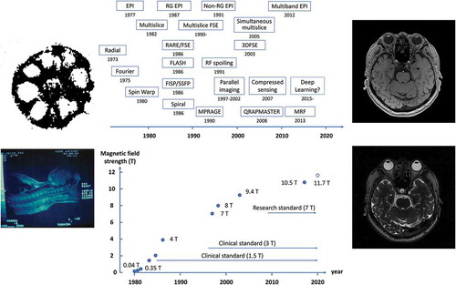
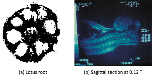
Figure 1 (a) shows a cross-sectional magnetic resonance (MR) image of lotus root acquired in 1979 in the Institute for Solid State Physics (ISSP), University of Tokyo. This image was reconstructed from projections of the lotus root measured using a continuous wave NMR instrument. I saw the image in the newspaper when I was in the final year of my doctoral course in physics and decided to join Toshiba company, because the ISSP was working with Toshiba. Figure 1 (b) shows a sagittal cross-section of my upper body acquired in 1982. This image was acquired in a 0.12 T static magnetic field using a body RF coil that I made by myself. The body coil was a saddle-shaped RF coil with an opening of 35 cm high and 45 cm wide using 3.0 mm diameter Cu wire. It was easy to make such a body coil because the wavelength of the RF wave was very long (about 60 m) compared to the size of the body.

Figure 1. (a) A cross-sectional image of lotus root measured by continuous wave NMR and the projection method acquired in 1979. It was measured by Dr. Kozo Sato (University of Tokyo) and reconstructed by Dr. Tamon Inouye (Toshiba). The static magnetic field strength was 0.4 T. The number of projections was 36 per 180 degrees. (b) The author’s sagittal image acquired by the projection method on 5 August 1982, using a 0.12 T air-core electromagnet at Toshiba Central Hospital in Tokyo. This image was reconstructed from 180 projection data acquired with a spin-echo sequence (TR = 400 ms). The measurement time was 9 minutes and 36 seconds

In those days, several groups were developing whole-body MRI systems in various places of the world. At Hammersmith Hospital in England, a system was constructed using a projection reconstruction method in a 0.15 T magnetic field with a superconducting magnet, and many clinical images were reported [6]. In the United States, the development of MRI systems was performed at the University of California, San Francisco and other institutions, and in 1981, UCSF reported clear images acquired with the multislice and multiple spin-echo technique at 0.35 T [7]. This multislice spin-echo technique formed the framework of the current clinical MRI. The static magnetic field of 0.35 T was more than twice as large as that reported in previous studies and triggered an increase in the magnetic field of MRI. This is because the signal-to-noise ratio of the human MR image increases proportional to the static magnetic field strength. Subsequent growth in the static field strength of the whole-body MRI systems are shown in Figure 2.

Figure 2. Changes in static magnetic field strength in whole-body MRI systems. The 1.5 T MRI became the clinical standard in the late 1980s, and the 3 T MRI became the clinical standard around the year 2000

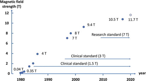
About 2 years after UCSF announced the 0.35 T MRI, General Electric (GE) company announced an MRI using a 1.5 T magnetic field [8]. After about a year of debate to determine the optimal magnetic field for MRI (‘field strength war’), 1.5 T became the standard magnetic field for clinical MRI. In the year of 2000 or so, 3 T became the next standard magnetic field for clinical MRI, and in 2017, a clinical MRI with a field of 7 T received FDA (Food and Drug Administration, USA) and CE (Conformité Européenne) approvals. Much higher field MRI systems are used for research purposes (9.4 T, 10.5 T, 11.7 T) [9–11].

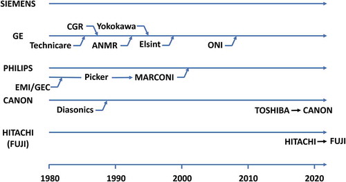
Figure 3 shows a history of the current top five whole-body MRI manufacturers. Siemens, the current leader, has never done any mergers and acquisitions, which is in sharp contrast to GE, which has repeated it many times. TOSHIBA and HITACHI, which have been two major Japanese MRI manufacturers for a long time, have recently transferred their medical imaging systems divisions to CANON and FUJI Film.

Figure 3. History of merge and acquisition of top 5 whole-body MRI venders. Recently, medical imaging divisions of Toshiba and Hitachi were acquired by Canon and Fuji film. More than 10 venders are shipping clinical whole-body MRI systems in China (not shown)

Before introducing the history and current status of MRI technology, images taken with the latest ‘routine’ clinical MRI sequences are described in Figure 4. Figure 4 (a)–(g) show images of my head acquired with a state-of-the-art 3 T MRI system (SIGNA, Premier, GE Healthcare, Waukesha, WI, USA) using multislice or three-dimensional (3D) imaging techniques. Figure 4 (a) is a T₁ weighted fast spin-echo (FSE) image, in which the tissue with a longer T₁ gives lower image intensity. Figure 4 (b) is a T₂ weighted FSE image, in which the tissue with a longer T₂ gives higher image intensity. Figure 4 (c) is an image obtained by the FLAIR (fluid-induced inversion recovery) method, which is a T₂ weighted FSE image with cerebrospinal fluid signal suppression, which is very useful for diagnosis of brain disease. Figure 4 (d) is acquired with a method called MPRAGE (magnetization prepared rapid gradient echo), which is a 3D T₁ weighted method used for segmentation of white matter and gray matter. Figure 4 (e) shows the axial section imaged by a 3D FSE sequence with 110 ms echo time (TE). Figure 4 (f) is a T₂* weighted image used for quantitative susceptibility mapping (QSM). Figure 4 (g) is acquired with a diffusion-weighted image, which is useful for early detection of cerebral infarction. Figure 4 (h) is an MR angiography image, which is used to detect vascular abnormalities.

Figure 4. Typical clinical MR images of the author’s brain acquired at 3 T in 2019. The pulse sequences were (a) T₁ weighted fast spin echo (FSE) (TR/TE = 550 ms/8.7 ms), (b) T₂ weighted FSE (TR/TE = 5272 ms/103 ms), (c) Fluid attenuated inversion recovery (FLAIR) (TR/TI/TE = 8000 ms/2348 ms/143 ms), (d) Magnetization prepared rapid gradient echo (MPRAGE) (TR/TI/TE/FA = 8000 ms/1873 ms/2.88 ms/6°), (e) T₂ weighted 3D FSE (TR/TE = 2252 ms/110 ms), (f) T₂* weighted gradient echo (TR/TE/FA = 30 ms/20.34 ms/5°), (g) diffusion weighted imaging (TR/TE = 3000 ms/80 ms, b = 1000), and (h) time of flight MR angiography (TR/TE/FA = 20 ms/3.4 ms/18°)

In the following section, I will describe the MRI hardware, MRI data acquisition, and MRI application that produced the images shown in Figure 4, and MRI simulation that can reproduce any MR images.

2. MRI hardware

2.1 System overview

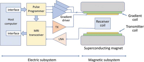
Figure 5 shows the current standard configuration of the whole-body MRI system [12], which consists of a magnet, a magnetic-field gradient coil set, and RF coils, which house the patient, and the part that supplies power to these coils and processes the detected signal. The former part (various types of coils) can be called a ‘magnetic subsystem’ because it generates various types of magnetic fields and interacts magnetically with the nuclear spins of the subject. The latter part can be called an ‘electric subsystem’ because it supplies control signals and drive power to the coils, and processes the detected MR signals. Since many review papers and textbooks have been written on magnets, gradient coils, and RF coils [13–16], this review will introduce the transceiver in detail [17], which is rarely published before.

Figure 5. A block diagram of the whole-body MRI system. The system can be divided into two subsystems; magnetic and electric subsystems

2.2 Magnet

There are three types of magnets used in the whole-body MRI system: superconducting magnets, permanent magnets, and resistive electromagnet magnets. The resistive electromagnet magnets were used only in the very early stage of the MRI development, and will not be described here. Therefore, only superconducting magnets and permanent magnets are described in this section.

Most superconducting magnets use a cylindrical cryostat, and the patient is inserted into the circular bore. In this case, both the magnetic-field gradient and RF coils are similarly cylindrical in shape. On the other hand, there are flat magnets split vertically to generate a vertical static magnetic field in the horizontal gap.

Most of the conductors for superconducting magnets are NbTi, and only a small part of them are made of materials such as Nb₃Sn and MgB₂ (superconducting critical temperature ~ 39 K, no liquid helium required). The advantages of NbTi wire are low cost (about one-tenth) compared to Nb₃Sn wire and attainable high magnetic-field strength (about 10 times) compared to MgB₂ wire. In addition, YBCO-based and Bi-based superconducting wires or tapes, which are high-temperature superconductors, are currently under development for the whole-body MRI systems.

　Currently, NdFeB-based materials [18] are used as permanent magnet materials of whole-body MRI systems. The shape is a so-called the vertical magnetic-field type, in which the magnetic poles are placed up and down and the gap are open horizontally. The static magnetic-field strength is 0.2 to 0.4 T.

Although some superconducting magnets for MRI have a vertical static field, almost all permanent magnets for MRI have a vertical static field. The MRI systems using these magnets, called open MRIs, usually have a lower static magnetic-field strength than cylindrical bore MRIs, but are more suitable for the examination of claustrophobic patients and children, and interventional use due to their superior openness.

2.3 Magnetic-field gradient coil

The magnetic-field gradient coil is a coil set that generates magnetic field along the static magnetic field that linearly change in the x, y, and z directions, respectively. The maximum strength and the rate of change of the gradient fields are important specifications for fast image acquisition. Therefore, in the early 1980s, the maximum strength was about 1 mT/m and the rise time to the maximum strength was about 1 ms, but with the current high-end models have a maximum strength of 40 mT/m to 100 mT/m and a rise time to the maximum strength of 0.2 to 0.3 ms. Regarding the rising speed of the gradient, a quantity called slew rate is defined, and the unit is mT/m/ms or T/m/s. For example, if the maximum intensity of 40 mT/m is reached in 0.2 ms, it is 200 mT/m/ms or 200 T/m/s. This slew rate is limited by peripheral nerve stimulation, which the US FDA guidelines set at 20 T/s for dB/dt.

The gradient coil is composed of two types of coils, primary and shielded coils, to generate a linear gradient magnetic field inside the coil and as small magnetic field as possible outside the coil [19]. However, since the leakage magnetic field cannot be completely reduced to zero, eddy currents are generated in the surrounding conductors, which affects the quality of the MR image. For this reason, pre-emphasis circuits are used to compensate the effects of eddy currents. In addition, a method has been developed to measure the impulse response of the gradient coil system and thereby perform image reconstruction [20].

2.4 RF coil

The RF coil consists of a transmitter coil and a receiver coil. The transmitter coil is used to apply an RF magnetic field to excite the subject’s nuclei. On the other hand, the receiver coil is used to detect the precession of the nuclei. In the early stages of MRI development, a coil for both transmission and reception was often used, and even now, a coil for both transmission and reception is sometimes used for the RF coil dedicated to the head. However, since the purpose of the transmitter coil and the purpose of the receiver coil are different, they are optimized separately as described below.

The transmitter coil, also called a volume coil, is designed for the purpose of uniformly exciting the entire subject. In many cases, birdcage coils are used [21]. In addition, MRI systems with a high magnetic field of 3 T or more use multiple transmitter coils to ensure that a uniform RF magnetic field penetrates into the subject. A transmitter of several tens of kW is used to drive the transmitter coil, but it is necessary to pay attention to the limitation by specific absorption rate (SAR).

　For the receiver coil, an array coil, which uses multiple receiver coils, are used to enable high sensitivity reception over a wide field of view (FOV) [22]. In addition, such multiple receiver coils are essential for parallel imaging. These receiver coils have been heavy and bulky for a long time, but recently they have become lighter and very flexible.

2.5 MRI transceiver

In the early days of MRI development, analog devices were used in all electrical systems except the computers and the pulse programmers. However, with the progress of digital devices, most of the analog devices inside the MRI systems have been replaced with digital devices. This change took place from the late 1980s to around the year of 2000, and digital transceivers are now used in all clinical MRI systems. However, there are many textbooks that assume the use of analog transceivers and many historical papers were written using them. Therefore, the analog transceiver and the digital transceiver are described, and a research comparing them using the same MRI system is introduced below [17,23].

Figure 6 shows the block diagrams ((a) and (b)) of the analog transceiver and the digital transceiver, respectively, and the photographs of the actual circuit boards ((c) and (d)).

Figure 6. (a) Block diagram of the analog transceiver, (b) block diagram of the digital transceiver, (c) analog transceiver board, (d) digital transceiver board. The transceiver boards were developed by MRTechnology Inc. (Tsukuba, Japan)

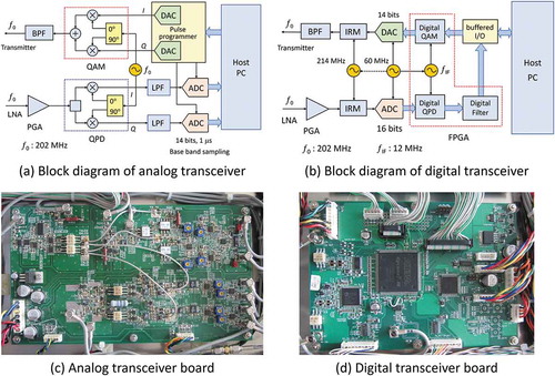
In the analog transceiver, the RF pulse waveform is output as an analog waveform from the pulse programmer controlled by the host computer via a DA converter, and it undergoes quadrature amplitude modulation (QAM) using the carrier radio frequency of $f_0$. By the modulation, an RF pulse having an arbitrary phase and amplitude in the rotating frame is generated. On the other hand, the RF MR signal received by the RF coil is amplified and then quadrature phase-sensitive detection (QPD) is performed using the carrier radio frequency of $f_0$, and in-phase and out-of-phase signals that are orthogonal in the rotating frame are obtained. Since these signals may contain noise and unwanted signals outside the FOV, they are digitized after passing through a low pass filter (anti-aliasing filter) and stored in the host computer.

　In the digital transceiver, the digital data of the RF pulse shape given by the pulse programmer controlled by the host computer is supplied to the digital QAM modulator of the transceiver, and the RF pulse waveform is created by digital calculation. This QAM is performed in synchronization with the 12 MHz clock signal for the field-programmable gate array (FPGA). The output digital signal is converted with a clock of 60 MHz to generate an analog waveform of the RF pulse. The analog RF pulse waveform is up-converted to the Larmor frequency of 202 MHz via the image rejection modulator (IRM). The RF MR signal received by the RF coil is down-converted to an RF signal in the 12 MHz band by the IRM, then digitized at a clock frequency of 60 MHz and supplied to the digital QPD circuit. The detected signal is filtered by a digital filter and supplied to the host computer. The area surrounded by the red dotted line in Figure 6 (b) is implemented on the FPGA (shown in Figure 6 (d).

The images acquired with the identical hardware units except the transceivers are shown in the upper (analog) and lower (digital) rows of Figure 7. These images were central cross-sectional images selected from 3D image datasets of a kumquat acquired by a 3D spin-echo imaging sequence (TR/TE = 800 ms/20 ms) using a 4.74 T (202 MHz proton resonance frequency) vertical bore superconducting magnet (89 mm room temperature bore). In the analog transceiver, the dynamic range was expanded by using a dual scan method. Figure 7 (a) and (d) are images with a 40.96 mm FOV, and (b) and (e) are images with a reduced FOV. There are bright spots due to artifacts around DC in the images acquired with the analog transceiver, whereas they do not appear in the images acquired with the digital transceiver. The artifact is probably due to $1/f$ noise at very low frequencies. Also, as shown in Figure 7 (c) and (f), the ghost-like artifact in the phase encoding direction (vertical direction) observed by the analog transceiver are not observed by the digital transceiver. This is probably due to the instability of the transmit or receive phase in the analog transceiver.

Figure 7. (a) A 2D cross-section selected from a 3D image dataset (512 × 512 × 64 voxels) of a kumquat acquired with a 3D spin-echo sequence (TR/TE = 800 ms/20 ms) at 4.74 T using the analog transceiver. (b) The central part of the image (a). (c) The cross-section of (a) with a narrow display window. (d) A 2D cross-section selected from a 3D image dataset of the kumquat acquired with the digital transceiver under the same condition as (a). (e) The central part of the image (d). (f) The cross-section of (d) with a narrow display window

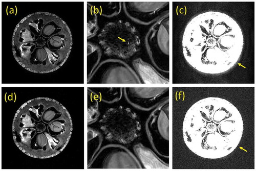
In this way, the digitization of the transceiver system in the history of MRI greatly contributed to improving the image quality of MR images.

3. MRI data acquisition

One of the major technological developments in MRI is the evolution of data collection methods. Conventional two-dimensional MR imaging is performed by scanning the Fourier space of an object repeatedly with a repetition time TR, which is set to be about the same as T₁ (~1 s) of living tissue protons. Acquisition is repeated by the number of phase encoding lines or number of pixels in the phase encoding direction (for example, 256), so that a single image is scanned in 256 seconds, or about 4 minutes. Therefore, it is necessary to speed up the imaging time to acquire high-quality images over the three-dimensional region of the object within a limited examination time (less than 5 minutes for one contrast image acquisition and less than 30 minutes for one patient examination). Fast image acquisition is even more important in the case of imaging of moving organs. Therefore, the history of MRI data collection methods focused on faster image acquisition is described below. Before that, I will explain the k-space, which is the basis of the data collection in MRI [24–27].

3.1 k-space trajectory

Consider the MR signal immediately after applying a 90° RF pulse to the nuclear magnetization distribution $M\left(x,y,z\right)$ generated in a static magnetic field B₀. The effect of relaxation times (T₁ and T₂) is ignored. After the excitation, when constant intensity gradients $G_x,G_y$, and $G_z$ are applied for $t_x,t_y$, and $t_z$ respectively, the MR signal becomes

(1) $S\left(t_x,t_y,t_z\right)\propto \int \int \int M\left(x,y,z\right)exp\left(-i\gamma G_{x}x{t}_x-i\gamma G_{y}y{t}_y-i\gamma G_{z}z{t}_z\right)dxdydz$(1)

where γ is the gyromagnetic ratio of the nucleus (this expression is a left-handed expression, and a right-handed expression with the sign of the phase term as + is sometimes used). Here, if we set $\gamma G_x{t}_x=2\pi k_x$, $\gamma G_y{t}_y=2\pi k_y$, and $\gamma G_z{t}_z=2\pi k_z$,

(2) $S\left(k_x,k_y,k_z\right)=\int \int \int M\left(x,y,z\right)exp\left(-i2\pi k_{x}x-i2\pi k_{y}y-i2\pi k_{z}z\right)dxdydz$(2)

where the proportionality constant is set to 1. Since the MR signal $S\left(k_x,k_y,k_z\right)$ is the Fourier component of the nuclear magnetization $M\left(x,y,z\right)$, the nuclear magnetization is

(3) $M\left(x,y,z\right)=\int \int \int S\left(k_x,k_y,k_z\right)exp\left(i2\pi k_{x}x+i2\pi k_y+i2\pi k_z\right)d{k}_{x}d{k}_{y}d{k}_z$(3)

That is, the nuclear magnetization distribution can be represented by the inverse Fourier transform of the measured signal. This is the principle of the Fourier imaging method in MRI [5].

　$G_x$, $G_y$, and $G_z$ shown above can be varied over time and $k_x$, $k_y$, and $k_z$ can be generally defined as

$k_x\left(t\right)=\frac{\gamma }{2\pi }\underset{0}{\overset{t}{\int }}{G}_x\left(u\right)du$, $k_y\left(t\right)=\frac{\gamma }{2\pi }\underset{0}{\overset{t}{\int }}{G}_y\left(u\right)du$, $k_z\left(t\right)=\frac{\gamma }{2\pi }\underset{0}{\overset{t}{\int }}{G}_z\left(u\right)du$. (4)

That is, the motion of $\left(k_x\left(t\right),k_y\left(t\right),k_z\left(t\right)\right)$ in k-space can be designed freely by using time-varying gradient waveforms. This is the k-space trajectory. Using this idea, different imaging techniques can be understood and explained in a unified way [24–27].

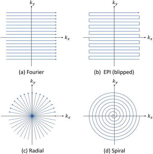
Figure 8 shows the trajectories of typical imaging methods. The most typical method of MRI by Ernst et al. is expressed as a large number of linear trajectories parallel to the coordinate axes of k-space [5]. Echo planar imaging (EPI), which is a typical example of ultrafast imaging method, is represented as one consecutive trajectory in k-space [28,29]. In addition, Lauterbur’s projection method, which was the first proposal for MRI, is expressed as a trajectory that passes through the origin of k-space and changes the angle with the coordinate axes at regular intervals [1]. A spiral trajectory has also been proposed that from the origin of the k-space toward the outside [30]. Sampling in the Cartesian coordinate system in k-space is called Cartesian sampling, and the other sampling is called Non-Cartesian sampling. The image reconstruction by Cartesian sampling is performed by a multidimensional FFT, and that by Non-Cartesian sampling is performed by a non-uniform FFT (NU-FFT).

Figure 8. K-space trajectory in MRI. (a) Fourier imaging. (b) Echo planar imaging. (c) Radial. (d) Spiral

3.2 Fast imaging

Figure 9 shows the history of data collection in MRI. The history is explained according to this figure below.

Figure 9. History of data acquisition in MRI. The main motivation for the MR data acquisition was fast image acquisition. The year shown below the sequence name is that the first report was published

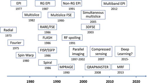
　As mentioned before, the first method proposed by Lauterbur was the radial method [1]. Shortly thereafter, Ernst et al. proposed the first Cartesian sampling method, Fourier imaging [3]. The Fourier imaging, combined with the selective excitation method and the gradient echo method for signal readout, has resulted in the spin warp method and became the standard signal acquisition method [4]. Furthermore, by combining this method with the spin-echo and multislice methods, the multislice spin-echo method was established, which became the standard imaging method for clinical imaging [6].

　On the other hand, the echo-planar imaging method by Mansfield was proposed in 1977 [28], but the hardware hurdle to realize it was extremely high. By employing a resonant gradient coil set, whole-body EPI images were successfully acquired in 1987 [31]. However, since conventional imaging was not possible with the resonant gradient coil set, EPI with a non-resonant gradient coil set was attempted [32], and subsequently EPI could be performed with normal clinical MRI systems. The progress of the gradient coil system for EPI also promoted improvements of other pulse sequences.

　After the multislice spin-echo method was established as a standard imaging method [7], no innovative techniques were developed for some time, but in the mid-1980s, new imaging techniques such as FLASH [33,34], FISP [35], RARE [36] and Spiral [30] were proposed. In particular, FLASH increased the speed of previous spin-echo imaging methods by more than 10 times, and the introduction of the RF spoiling method [37] led to the establishment of a fast T₁-weighted imaging method. The RARE method (fast spin-echo (FSE) method) using multiple spin-echo replaced all conventional spin-echo imaging methods in clinical imaging. As a result, the standard sequence for clinical use became T₁ weighted, T₂ weighted, and FLAIR multislice FSE sequences.

During the 1980s, new proposals for k-space scanning type high-speed imaging were completed, but in the late 1990s, parallel imaging methods such as SMASH [38], SENSE [39], and GRAPPA [40] were proposed. These methods reduced the number of scans in k-space by using the sensitivity distributions of multiple receiver coils as positional information, and achieved more than twice the speed of conventional imaging methods. Then, in 2007, a compressed sensing method was proposed that can omit the number of samples in k-space, making it possible to further speed up the imaging process [41]. After 2015, the deep learning method has begun to influence the way MRI scans are performed.

In addition, QRAPMASTER [42] and MR fingerprinting [43], in which multiple NMR parameters such as proton density, T₁, T₂, etc. are efficiently obtained simultaneously, have been proposed and are widely used as a promising method for quantitative imaging.

4. MRI applications: new image contrasts

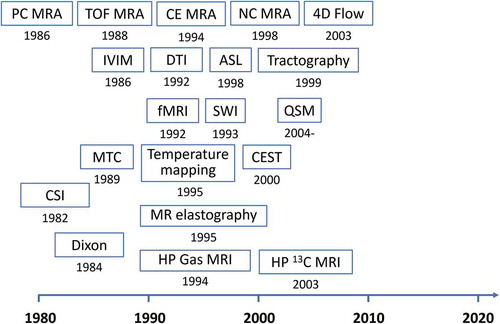
The history of MRI technology development was not only the history of fast imaging, but also the history of how to acquire new image contrast. The history is shown in Figure 10, and the contents are outlined below.

Figure 10. History of new image contrasts in MRI. The year shown below the title is that the first report was published

4.1. MR angiography and macroscopic flow measurements

As shown in Figure 4 (h), MR angiography of the brain vessels is one of the routine clinical examinations. MR imaging of the vascular system has attracted great attention from the early stage of the MRI development, and several practical methods have been reported.

The first practical method was phase-contrast angiography (3D PC MRA), which visualizes the vasculature using the phase shift of the precession of the nuclear magnetization generated as blood protons move through the magnetic-field gradient [44]. On the other hand, time of flight MR angiography (TOF MRA) was developed using the inflow effect [45] and became the standard method for brain MRA. This was because this technique reduced measurement time by using only the intensity of nuclear magnetization, avoided problems such as phase aliasing, and the use of the maximum intensity projection method facilitated the visualization of 3D structures of the vascular system.

One of the main features of MRI was no need to use contrast agents, but contrast-enhanced MRA (CE MRA) was proposed in 1994 to dynamically visualize the vessels of the arterial system by actively using contrast agents that shorten T₁ [46]. This is largely due to the fact that 3D T₁ weighted imaging can be performed at high speed. On the other hand, for relatively slow flow, such as the vasculature of the lower extremities, a method that allows excellent visualization without the use of contrast agent was proposed and is called non-contrast enhanced MRA (NC MRA) [47].

The 3D PC MRA has fallen out of use for a while because of its longer measurement time comparing with TOF MRA, but has been used as a 2D flow measurement method called 2D-phase contrast MRI. Furthermore, the 3D PC MRA has been developed into 4D flow MRI, which is a quantitative blood flow vector measurement method that includes information on the cardiac cycles, by incorporating advanced imaging techniques such as parallel imaging and compressed sensing [48].

4.2. Cardiac MRI

Cardiac MRI forms a unique area in MRI [49]. This is because the heart is always moving, and the imaging techniques used in other regions cannot be used in the same way. In cardiac MRI, morphology, function, and viability of the heart are assessed. To evaluate the morphology of the heart, the balanced SSFP sequence with retrospective gating is the fundamental technque for imaging. Spatial tagging sequences are frequently used. Since the measurement of T₁ and T₂ of moving organs is performed, many original pulse sequences for the heart have been reported.

4.3. Microscopic molecular motion and flow

In biological tissues, not only the macroscopic flows such as blood flow described above, but also microscopic flows within capillaries and the diffusion of water molecules within and outside of cells affect the MR signal. However, it is difficult to visualize and discriminate these microscopic motions as long as they are imaged with a resolution of about 1 mm cube. To solve this problem, in 1986, Le Bihan named these phenomena intravoxel incoherent motion (IVIM), defined the apparent diffusion coefficient, and described the phenomenon [50].

On the other hand, Basser, who had doubts about the diversity of diffusion measurements in vivo, thought that diffusion coefficients should be expressed in terms of tensors, and reported the formulation, measurement methods, and experimental results [51,52]. The diffusion tensor has received significant attention as a tractography, visualizing nerve fibers in the white matter of the brain [53,54].

Dynamic susceptibility contrast (DSC) MRI using Gd contrast agents and arterial spin labeling (ASL) MRI [55], which quantify brain perfusion, were also proposed around this time.

4.4. Magnetically related contrasts

In 1990, Ogawa et al. found that imaging of mouse brains in high magnetic fields with T₂* weighted gradient echo sequences resulted in a significant change in signal intensity depending on the oxygenation state of the blood, which they attributed to the paramagnetic deoxyhemoglobin [56]. This contrast (BOLD contrast) enabled functional brain mapping using T₂* weighted gradient echo images [57].

On the other hand, susceptibility-weighted imaging (SWI), which used T₂* weighted images to emphasize the magnetic susceptibility, was proposed in 1993, which utilized the paramagnetism of venous blood [58,59]. Furthermore, quantitative susceptibility mapping (QSM) was proposed to quantify the magnetic susceptibility distribution, and it is still actively studied [60–62].

4.5 Molecular structure related contrast

Although the main target of MRI is protons of water molecules, chemical shift imaging is a general measurement technique that focuses on the nuclei of other molecules [25]. In this method, position is identified by phase encoding with gradients, and signal observation is performed without gradients. This method is widely used for mapping brain metabolites. On the other hand, the Dixon’s method was proposed in 1984 as a method for separating water and fat protons found in various tissues of the human body [63], and its improved version was later published [64].

A technique called magnetization transfer (MT) contrast is used to image the relationship between the protons of free water molecules and those of other molecules [65]. This is a method to visualize the relationship between the protons of macromolecules and those of free water. In this method, the magnetization transfer ratio contrast is obtained by measuring the difference between images acquired by the radio-frequency irradiation at the resonance frequency of the macromolecular protons, and far off-resonance 10 or more kHz. Furthermore, in 2003, it was found that the pH distribution can be visualized by measuring the MT effect in amide proton (-NH) in vivo, which is called the chemical exchange saturation transfer (CEST) method and is used to visualize tumors [66].

4.6. Hyperpolarized nuclei

The rate of nuclear spin polarization used for MRI is about 0.001% at room temperature in the direction of the static field, even when the magnetic field is 1.5 T for protons. However, by irradiating ³He and ¹²⁹Xe gases mixed with alkali metal gases (Rb⁺) with a circularly polarized laser light (795 nm wavelength), the polarization of their nuclei can be dramatically enhanced by up to a few 10% (hyperpolarization). A study using ¹²⁹Xe was reported in 1994 [67], and a study using ³He was reported in 1995 [68]. These are mainly used for imaging of the lung air space.

In an alternative approach, studies have been reported to transfer the magnetization of the electron spins of para-hydrogen at low temperatures to the ¹³C nucleus and administer the drug containing it to visualize its metabolism [69].

4.7. Other physical parameters

Examples of mapping other physical parameters are the mapping of temperature and that of elastic modulus. Although temperature mapping methods using various NMR parameters have been considered, the most popular method is currently the one that measures the phase change of the water proton signal with in a gradient echo sequence [70]. The elastic modulus was visualized by detecting a phase shift due to a gradient waveform synchronized with the period of an externally applied elastic wave [71]. Both methods take advantage of the features of MRI, which measures physical quantities non-invasively.

5. MRI simulation

In MRI, as in other fields, various types of computer simulations are being performed. Among them, a so-called first-principles calculation method, which tries to reproduce the entire imaging process of MR images from the basic equations such as the Bloch equations [72], has recently attracted much attention. The reason for this is that in recent years this has become a reality due to the dramatic increase in computing power. We briefly introduce the principles of MRI simulator [73–75], and then introduce the history of various implementations.

5.1 Principle of the MRI simulator

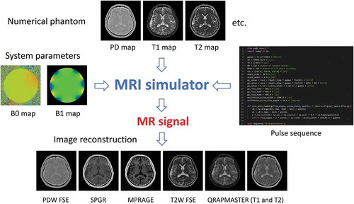
Figure 11 describes the principle of the MRI simulator. The MRI simulator requires numerical phantom (object model) files that model the subject, system parameter files describing the MRI system hardware, and a pulse sequence file describing the operation of the pulse sequence. The MRI simulator program interprets the pulse sequence described in the pulse sequence file and calculates the motion of the nuclear magnetization (isochromat) at each time according to the Bloch equations corresponding to each event. Then, the MR signal is calculated by summing up the transverse components of the nuclear magnetization $M_x$ and $M_y$ in the rotating frame over the whole subject. The MRI simulator calculates the MR signal for the large amount of nuclear magnetization that composes the entire subject, but it is based on a temporal change of a single nuclear magnetization vector $\vec{M}={\left(M_x,M_y,M_z\right)}^T$.

Figure 11. Schematic view of the MRI simulator. The MRI simulator requires three input files: numerical phantoms, system parameters, and a pulse sequence

The nuclear magnetization varies according to the Bloch equation, which can be written in the rotating frame as follows:

$\frac{d\vec{M}}{dt}$ $=\gamma \vec{M}\times {\vec{B}}_e-\left(\begin{array}{c}{M}_x/T_2\\ M_y/T_2\\ \left(M_z-M_0\right)/T_1\end{array}\right)$, (5)

where, γ is the gyromagnetic ratio of the nuclei, ${\vec{B}}_e$ is the effective magnetic field in the rotating frame, and $T_1$ and $T_2$ are longitudinal and transverse relaxation times of the nuclear magnetization, $M_0$ is magnitude of the magnetization vector at the thermal equilibrium. ${\vec{B}}_e$ can be expressed as

(6) ${\vec{B}}_e\left(t\right)=\mathrm{\Delta }{B}_0\left(x,y,z\right)\hat{z}+\left(G_x\left(t\right)x+G_y\left(t\right)y+G_z\left(t\right)z\right)\hat{z}+B_{1x}\left(t\right)\hat{x}+B_{1y}\left(t\right)\hat{y}$(6)

where $\mathrm{\Delta }{B}_0$ is inhomogeneity of the static magnetic field, $G_x\left(t\right)$, $G_x\left(t\right)$, and $G_x\left(t\right)$ are magnetic field gradients, and $B_{1x}\left(t\right)$ and $B_{1y}\left(t\right)$ are two orthogonal components of radio frequency magnetic fields in the rotating frame.

To solve this equation numerically, set a time step ∆t and calculate the amount of change in the nuclear magnetization vector during ∆t. In addition, it is efficient to calculate the change due to the RF pulse and the change due to the relaxation effect separately. Each method is described below.

The RF pulse with arbitrary shape can be approximated as a set of short rectangular pulses with a width of ∆t. That is, the vector $\left(b_x,b_y,b_z\right)$ representing the rotation during ∆t, and the rotation angle θ are set as follows:

(7) $\theta =\sqrt{b_x^2+b_y^2+b_z^2},\theta =\sqrt{b_x^2+b_y^2+b_z^2}$(7)

(8) $\left(n_x,n_y,n_z\right)=\left(b_x,b_y,b_z\right)/\theta$(8)

where $\left(n_x,n_y,n_z\right)$ is a unit vector parallel to ${\vec{B}}_e$. The rotation matrix $R$ for the nuclear magnetization $\vec{M}$ by the short RF pulse is from the Rodrigues’ rotation formula as

(9) $R=\text{break}\left(\begin{array}{ccc}{n}_x^2\left(1-cos\theta \right)+{\theta }^{2}cos\theta & n_x{n}_y\left(1-cos\theta \right)-\theta n_{z}sin\theta & n_x{n}_z\left(1-cos\theta \right)+\theta n_{y}sin\theta \\ n_x{n}_y\left(1-cos\theta \right)+\theta n_{z}sin\theta & n_y^2\left(1-cos\theta \right)+{\theta }^{2}cos\theta & n_y{n}_z\left(1-cos\theta \right)-\theta n_{x}sin\theta \\ n_x{n}_z\left(1-cos\theta \right)-\theta n_{y}sin\theta & n_y{n}_z\left(1-cos\theta \right)+\theta n_{x}sin\theta & n_z^2\left(1-cos\theta \right)+{\theta }^{2}cos\theta \end{array}\right)$(9)

On the other hand, the change in the nuclear magnetization caused by the relaxation effect is

(10) $\left(\begin{array}{c}{M}_x\left(t+\mathrm{\Delta }t\right)\\ M_y\left(t+\mathrm{\Delta }t\right)\\ M_z\left(t+\mathrm{\Delta }t\right)\end{array}\right)=\left(\begin{array}{ccc}{E}_{2}cos\phi & -E_{2}sin\phi & 0\\ E_{2}sin\phi & E_{2}cos\phi & 0\\ 0& 0& 1\end{array}\right)\left(\begin{array}{c}{M}_x\left(t\right)\\ M_y\left(t\right)\\ M_z\left(t\right)\end{array}\right)+\left(\begin{array}{c}0\\ 0\\ 1-E_1\end{array}\right)M_0$(10)

where $E_1=\mathrm{e}\mathrm{x}\mathrm{p}\left(-\mathrm{\Delta }t/T_1\right)$ and $E_2=\mathrm{e}\mathrm{x}\mathrm{p}\left(-\mathrm{\Delta }t/T_2\right)$, and $\phi$ is defined as follows:

(11) $\phi =\gamma \underset{t}{\overset{t+\mathrm{\Delta }t}{\int }}{\left({\vec{B}}_e\right)}_{z}dt$(11)

The relaxation effect during the application of the RF pulse is calculated by performing the operation shown in (10) before or after the application of the above rotation matrix in (9).

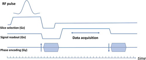
The above calculations are performed for all the nuclear magnetizations defined by the numerical phantom according to the pulse sequence shown in Figure 12. The MR signal can be obtained by calculating the sum of the transverse magnetization components for each sampling time in the data collection period.

Figure 12. A sequence chart of a currently typical gradient echo sequence. Typical time step for the calculation for the RF pulse event is 10 μs and that for data acquisition is 10 μs

In order to obtain simulated images comparable to real MR images, it is necessary to perform the above calculation for a large number of nuclear magnetizations (e.g. 256³ isochromats). In addition, if (1) phase dispersion in the voxel exceeds π radian due to inhomogeneity of the static magnetic field or gradient application for selective excitation, or (2) a large phase dispersion exist in the voxel due to TR shorter than T₂, a single voxel should be further divided into subvoxels and place a nuclear magnetization in each of them (of course, this is the same operation as placing multiple nuclear magnetizations in a single voxel).

The use of fast computers is necessary to perform such calculations. In the case of using CPUs multi-threaded computations are required, and the use of graphics processor units (GPUs) are extremely useful [73,74,76]. However, a variety of optimizations in programming are essential to increase the computation speed.

Figure 13 (a) shows cross-sectional images (5 mm slice thickness) of T₂ weighted multislice FSE sequence calculated using the MRI simulator [73] from the head numerical phantom. The head numerical phantom (T₁, T₂, and proton density) was created from the MR data acquired at 3 T (256³ pixels, voxel size: 0.86 mm × 0.86 mm × 1.0 mm) as shown in Figure 4. Figure 13 (b) and (c) show cross-sectional images at identical position obtained by the MRI simulation and the MR measurements. Although the conditions for the simulation and the measurement are slightly different, almost the same image is obtained in the simulated image except for detailed description.

Figure 13. (a) 2D cross-sections simulated with the T₂ weighted multislice FSE sequence (TR = 4800 ms, TE = 96 ms, echo train length (ETL) = 8, echo spacing = 12 ms). The images were calculated from 51,823,104 isochromats using BlochSolver [73]. The computation time was about 24 minutes using a GPU (GeForce RTX 2080Ti, NVIDIA, Santa Clara, USA). (b) The 2D cross-section selected from the multislice FSE images of (a). (c) The 2D cross-section selected from the image dataset acquired with the T₂ weighted multislice FSE sequence (TR = 5272 ms, TE = 103 ms, ETL = 20) at 3 T

5.2 Historical overview of MRI simulators

The MRI simulator has been proposed since the early 1980s, when MRI was first commercialized, and various MRI simulators have been proposed over time. The basic formulations have not changed much from that described in the previous section, but major change is the performance of the hardware. That is, as shown in Figure 14, an IBM 370 mainframe computer was used in a paper published in 1984 [77] and a VAX-11 super mini-computer was used in a paper published in 1986 [78]. A paper published in 1995 [79] used a PC with an intel 486 CPU, and a paper published in 1999 [80] used a workstation from Silicon Graphics International Corp.

Figure 14. History of MRI simulator programs and their typical computer systems. ODIN [81], SIMRI [82], JEMRIS [83], and MRiLab [84] are open source software. Compiled version of MRISIMUL [76], PSUdoMRI [85], and BlochSolver [73] are available from the web

After the year 2000, with the increase in CPU clock frequency and parallel computing using computer clustering and multi-core CPUs, practical MRI simulator programs have been published and have come to be used as open-source software [81–84]. These programs have been used in many studies and many research papers have been published. There are also published programs that are not open source but whose executable programs are available [73,76,85] from the web. Furthermore, recently, several MRI simulators compatible with GPUs has been published [73,76,84], and as shown in Figure 13, images with an image quality similar to that of real images are obtained.

Most current MRI simulators can reproduce relaxation time contrast and static magnetic-field inhomogeneity artifacts, in addition, some MRI simulators also can visualize diffusion effect [73,86], flow [87,88], and magnetization transfer effect [84], specific absorption rate [85], etc. In the future, it is expected that various MRI parameters can be visualized by speeding up the MRI simulator and developing numerical phantoms (object models).

6. Conclusion

The history of MRI for about 50 years was reviewed from various perspectives. MRI has been developed not only by clinical medicine but also by the contributions of researchers and engineers in various fields such as mathematics, physics, chemistry, biology, information science, and electronic engineering. MRI is an indispensable examination modality in clinical medicine, and is an attractive measurement technology with various possibilities. In addition, although not mentioned in this review, the application of MRI to other than clinical medicine is also widely performed. Many researchers are still actively engaged in MRI research, and further development is expected in the future.

Disclosure statement

The author is a director of MRIsimuations Inc.

References

- Lauterbur PC. Image formation by local induced interactions: examples employing nuclear magnetic resonance. Nature. 1973;242:190–26.
- Damadian R. Tumor detection by nuclear magnetic resonance. Science. 1971 Mar 19;171:1151–1153. .
- Edelstein WA, Hutchison JMS, Johnson G, et al. Spin warp NMR imaging and applications to human whole-body imaging. Phys Med Biol. 1980;25:751–756.
- Garroway AN, Grannell PK, Mansfield P. Image formation in NMR by a selective irradiative process. J Phys. 1974;C7:L457–462.
- Kumar A, Welti D, Ernst RR. NMR Fourier Zeugmatography. J Magn Reson. 1975;18:69–83.
- Bydder GM, Steiner RE, Young IR, et al. Clinical NMR imaging of the brain: 140 cases. AJR Am J Roentgenol. 1982;139:215–236.
- Crooks LE, Arakawa M, Hoenninger J, et al. Nuclear magnetic resonance whole-body imager operating at 3.5 K gauss. Radiology. 1982;143:169–174.
- Hart HR, Bottomley PA, Edelstein WA, et al. Nuclear Magnetic Resonance Imaging: contrast-to-Noise Ratio as a Function of Strength of Magnetic Field. AJR. 1983;141:1195–1201.
- Ugurbil K. Imaging at ultrahigh magnetic fields: history, challenges, and solutions. Neuroimage. 2018;168:7–32.
- Sadeghi-Tarakameh A, DelaBarre L, Lagore RL, et al. In vivo human head MRI at 10.5T: a radiofrequency safety study and preliminary imaging results. Magn Reson Med. 2020;84:484–496.
- Quettier L, Aubert G, Belorgey J, et al. Iseult/INUMAC whole body 11.7 T MRI magnet. IEEE Trans Appl Supercond. 2017;27:1–4.
- Kose K. Console electronics. educational lecture. Proc Intl Soc Magn Reson Med. 2013;21.
- Lvovsky Y, Stautner EW, Zhang T. Novel technologies and configurations of superconducting magnets for MRI. Supercond Sci Technol. 2013;26:93001.
- Moser E, Laistler E, Schmitt F, et al. Ultra-high field NMR and MRI – the role of magnet technology to increase sensitivity and specificity, Front. Phys. 2017;5:33.
- Winkler SA, Schmitt F, Landes H, et al. Gradient and shim technologies for ultra high field MRI. Neuroimage. 2018;168:59–70.
- Vaughan JT, Griffith JR, editors. RF coils for MRI. UK: John Wiley & Sons; 2012.
- Hashimoto S, Kose K, Haishi T. Comparison of analog and digital transceiver systems for MR imaging. Magn Reson Med Sci. 2014;13:285–291.
- Sagawa M, Fujimura S, Togawa N, et al. New material for permanent magnets on a base of Nd and Fe. J Appl Phys. 1984;55:2083–2087.
- Mansfield P, Chapman B. Active Magnetic Screening of Gradient Coils in NMR Imaging. J Magn Reson. 1986;66:573–576.
- Vannesjo SJ, Haeberlin M, Kasper L, et al. Gradient system characterization by impulse response measurements with a dynamic field camera. Magn Reson Med. 2013;69:583–593.
- Hayes CE, Edelstein WA, Schenck JF, et al. An efficient, highly homogeneous radio frequency coil for whole-body NMR imaging at 1.5T. J Magn Reson. 1985;63:622–628.
- Roemer PB, Edelstein WA, Hayes CE, et al. The NMR phased array. Magn Reson Med. 1990;16:192–225.
- Hashimoto S, Kose K, Haishi T. Development of a pulse programmer for magnetic resonance imaging using a personal computer and a high-speed digital input–output board. Rev Sci Instrum. 2012;83:053702.
- Likes RS Moving gradient zeugmatography. US Patent #4307343 issued 22 Dec 1981.
- Brown TR, Kincaid BM, Ugurbil K. NMR chemical shift imaging in three dimensions. Proc Natl Acad Sci USA. 1982;79:3523–3526.
- Ljunggren S. A Simple Graphical representation of fourier-based imaging methods. J Magn Reson. 1983;54:338–343.
- Twieg DB. The k-trajectory formulation of the NMR imaging process with applications in analysis and synthesis of imaging methods. Med Phys. 1983;10:610–621.
- Mansfield P. Multi-planar Image Formation using NMR Spin Echoes. J Phys C: Solid State Phys. 1977;10:L55–58.
- Johnson G, Hutchison JMS. The limitation of NMR recalled echo imaging techniques. J Magn Res. 1985;63:14–30.
- Ahn CB, Kim JH, Cho ZH. High-Speed Spiral-Scan Echo Planar NMR Imaging – i. IEEE Trans Med Imaging. 1986;5:2–7. MI-5. .
- Rzedzian RR, Pykett IL. Instant Images of the Human Heart Using a New, Whole Body MR Imaging System. AJR. 1987;149:245–250.
- Souza SP, Roemer P, Peters S, et al. Echo-planar imaging with a non-resonant gradient power system. Proceedings of the 10th Annual Scientific Meeting of the SMRM, San Francisco, p 217.
- Hasse H, Frahm, Matthaei JD, Hanicke W, Merboldt KD. FLASH Imaging. Rapid NMR imaging using low flip-angle pulses. J Magn Reson. 1986;67:258–266.
- Frahm J, Haase A, Matthaei D. Rapid NMR imaging of dynamic processes using the FLASH technique. Magn Reson Med. 1986;3:321–327. .
- Oppelt A, Graumann R, Barfuß H, et al. FISP - a new fast MRI sequence. Electromedica. 1986;54:15–18.
- Hennig J, Nauerth A, Friedburg H, et al. Method for Clinical MR. Magn Reson Med. 1986;3:823–833.
- Zur Y, Wood ML, Neuringer LJ. Spoiling of transverse magnetization in steady-state sequences, Magn. Reson Med. 1991;21:251–263.
- Sodickson DK, Manning WJ; Sodickson DK, Manning WJ. Simultaneous acquisition of spatial harmonics (SMASH): fast imaging with radiofrequency coil arrays. Magn Reson Med. 1997;38:591–603.
- Prussmann KP, Weiger M, Scheidegger MB, et al. SENSE: sensitivity encoding for fast MRI. Magn Reson Med. 1999;42:952–962.
- Griswold MA, Jakob PM, Heidemann RM, et al. Generalized autocalibrating partially parallel acquisitions (GRAPPA). Magn Reson Med. 2002;47:1202–1210.
- Lustig M, Donoho D, Pauly JM. Sparse MRI: the application of compressed sensing for rapid MR imaging. Magn Reson Med. 2007;58:1182–1195.
- Warntjes JB, OD L, West J, et al. Rapid magnetic resonance quantification on the brain: optimization for clinical usage. Magn Reson Med. 2008;60:320–329. .
- Ma D, Gulani V, Seiberlich N, et al. MR Fingerprinting. Nature. 2013;495:187–192.
- Dumoulin CL, Hart HR. Magnetic resonance angiography. Radiology. 1986;161:717–720.
- Laub GA, Kaiser WA. MR angiography with gradient motion refocusing. J Compt Assit Tomogr. 1988;12:377–382. .
- Prince MR. Gadolinium-enhanced MR Aortography. Radiology. 1994;191:155–164.
- Miyazaki M, Sugiura S, Tateishi F, et al. Non-contrast-enhanced MR angiography using 3D ECG-synchronized half-Fourier fast spin echo. J Magn Reson Imaging. 2000;12:776–783.
- Markl M, Chan FP, Alley MT, et al. Time-resolved three-dimensional phase-contrast MRI. J Magn Reson Imaging. 2003;17:499–506.
- Lee DC, Markl M, Dall’Armellina E, et al. The growth and evolution of cardiovascular magnetic resonance: a 20-year history of the Society for Cardiovascular Magnetic Resonance (SCMR) annual scientific sessions. J Cardiovasc Magn Reson. 2018 Jan 31;20:8. .
- LeBihan D, Breton E, Lallemand D, et al. MR imaging of intravoxel incoherent motions: application to diffusion and perfusion in neurologic disorders. Radiology. 1986;161:401–407.
- Basser PJ, Mattiello J, LeBihan D. MR Diffusion Tensor Spectroscopy and Imaging. Biophys J. 1994;66:259–267.
- Basser PJ, Mattiello J, LeBihan D. Estimation of the effective self-diffusion tensor from the NMR spin echo. J Magn Reson. 1994;B103:247–254.
- Mori S, Crain BJ, Chacko VP, et al. Three-dimensional tracking of axonal projections in the brain by magnetic resonance imaging. Ann Neurol. 1999;45:265–269.
- Basser PJ, Pajevic S, Pierpaoli C, et al. In vivo fiber tractography using DT-MRI data. Magn Reson Med. 2000;44:625–632.
- Buxton RB, Frank LR, Wong EC, et al. A general kinetic model for quantitative perfusion imaging with arterial spin labeling. Magn Reson Med. 1998;40:383–396.
- Ogawa S, Lee TM, Kay AR, et al. Brain magnetic resonance imaging with contrast dependent on blood oxygenation. Proc Natl Acad Sci USA. 1990;87:9868–9872.
- Ogawa S, Tank DW, Menon R, et al. Intrinsic signal changes accompanying sensory stimulation: functional brain mapping with magnetic resonance imaging. Proc Natl Acad Sci USA. 1992;89:5951–5955.
- Haacke EM, Lai S, Yablonskiy DA, et al. In vivo validation of the bold mechanism: a review of signal changes in gradient echo functional MRI in the presence of flow. Int J Imaging Syst Technol. 1995;6:153–163. .
- Reichenbach JR, Venkatesan R, Schillinger DJ, et al. Small vessels in the human brain: MR venography with deoxyhemoglobin as an intrinsic contrast agent. Radiology. 1997;204:272–277.
- Li L, Leigh JS. Quantifying arbitrary magnetic susceptibility distributions with MR. Magn Reson Med. 2004;51:1077–1082.
- Liu T, Spincemaille P, de Rochefort L, et al. Calculation of susceptibility through multiple orientation sampling (COSMOS): a method for conditioning the inverse problem from measured magnetic field map to susceptibility source image in MRI. Magn Reson Med. 2009;61:196–204.
- Shmueli K, de Zwart JA, van Gelderen P, et al. Magnetic susceptibility mapping of brain tissue in vivo using MRI phase data. Magn Reson Med. 2009;62:1510–1522.
- Dixon WT. Simple proton spectroscopic imaging. Radiology. 1984;153:189–194.
- Glover GH, Schneider E. Three-point Dixon technique for true water/fat decomposition with B0 inhomogeneity correction. Magn Reson Med. 1991;18:371–383.
- Wolff SD, Balaban RS. Magnetization transfer contrast (MTC) and tissue water proton relaxation in vivo. Magn Reson Med. 1989;10:135–144.
- Zhou J, Payen JF, Wilson DA, et al. Using the amide proton signals of intracellular proteins and peptides to detect pH effects in MRI. Nat Med. 2003;9:1085–1090.
- Albert MS, Cates GD, Driehuys B, et al. Biological magnetic resonance imaging using laser-polarized 129Xe. Nature. 1994;370:199–201.
- Middleton H, Black RD, Saam B, et al. MR imaging with hyperpolarized 3He Gas. Magn Reson Med. 1995;33:271–275.
- Ardenkjaer-Larsen JH, Fridlund B, Gram A; Ardenkjaer-Larsen JH, Fridlund B, Gram A, et al. Increase in signal-to-noise ratio of > 10,000 times in liquid-state NMR. Proc Natl Acad Sci USA. 2003;100:10158–10163.
- Ishihara Y, Calderon A, Watanabe H, et al. A precise and fast temperature mapping using water proton chemical shift. Magn Reson Med. 1995;34:814–823.
- Muthupillai R, Lomas DJ, Rossman PJ, et al. Magnetic resonance elastography by direct visualization of propagating acoustic strain waves. Science. 1995;269:1854–1857.
- Bloch F. Nuclear induction, Phys. Rev. 1946;70:460–473.
- Kose R, Kose K. BlochSolver: a GPU-optimized fast 3D MRI simulator for experimentally compatible pulse sequences. J Magn Reson. 2017;281:51–65.
- Kose R, Setoi A, Kose K. A fast GPU-optimized 3D MRI simulator for arbitrary k-space sampling. Magn Reson Med Sci. 2019;18:208–218.
- Kose R, Kose K. Python pulse sequence development kit for a fast MRI simulator. Proc Intl Soc Magn Reson Med. 2020;28:3647.
- Xanthis CG, Venetis IE, Chalkias AV, et al. MRISIMUL: a GPU-based parallel approach to MRI simulations, IEEE Trans. Med Imaging. 2014;33:607–616. .
- Bittoun J, Taquin J, Sauzade M. A computer algorithm for the simulation of any nuclear magnetic resonance (NMR) imaging method, Magn. Reson Imaging. 1984;2:113–120. .
- Summers RM, Axel L, Israel S. A computer simulation of nuclear magnetic resonance imaging, Magn. Reson Med. 1986;3:363–376.
- Olsson MBE, Wirestam R, Persson BRR. A computer simulation program for MR Imaging: application to RF and static magnetic-field imperfections. Magn Reson Med. 1995;34:612–617.
- Kwan RK, Evans AC, Pike GB. MRI simulation-based evaluation of image-processing and classification methods. IEEE Trans Med Imaging. 1999;18:1085–1097.
- Jochimsen TH, von Mengershausen M. ODIN-object-oriented development interface for NMR. J Magn Reson. 2004;170:67–78.
- Benoit-Cattina H, Collewet G, Belaroussi B, et al. The SIMRI project: a versatile and interactive MRI simulator, J. Magn Reson. 2005;173:97–115. .
- Stöcker T, Vahedipour K, Pflugfelder D, et al. High-performance computing MRI simulations, Magn. Reson Med. 2010;64:186–193.
- Liu F, Velikina JV, Block WF, et al. Fast realistic MRI simulations based on generalized multi-pool exchange tissue model. IEEE Trans Med Imaging. 2017;36:527–537.
- Cao Z, Oh S, Sica CT, et al. Bloch-based MRI system simulator considering realistic electromagnetic fields for calculation of signal, noise, and specific absorption rate, Magn. Reson Med. 2014;72:237–247.
- Jochimsen TH, Schäfer A, Bammer R, et al. Efficient simulation of magnetic resonance imaging with Bloch-Torrey equations using intra-voxel magnetization gradients. J Magn Reson. 2006;180:29–38.
- Xanthis CG, Venetis IE, Aletras AH. High performance MRI simulations of motion on multi-GPU systems. J Cardiovasc Magn Reson. 2014;16:48.
- Fortin A, Salmon S, Baruthio J, et al. Flow MRI simulation in complex 3D geometries: application to the cerebral venous network. Magn Reson Med. 2018;80:1655–1665.