Advances toward fieldable atom interferometers

ABSTRACT

We review the field of atom interferometer inertial sensors. We begin by reviewing the path integral formulation of atom interferometers and then specialize the treatment to light-pulse atom interferometers and, in particular, gravimeters and gyroscopes. The bulk of the article focuses on the most common type of atom interferometer – the light-pulse interferometer, where the atom optics are composed of light pulses. Our article mainly focuses on a review of advances that aid in the practical implementation of atom interferometers toward gravimetry and inertial navigation. To that end, we develop a navigation model that aids in the connection of parameters and performance of atom interferometers to actual quantities of interest to the navigation community. Practical considerations of atomic inertial sensors, including dynamic range, bandwidth, dead time, and cross-coupling effects are discussed, before we review the field of accelerometer and gyroscope atom interferometers. Finally, we review advances in trapped-atom interferometers.

Graphical abstract

KEYWORDS:

• atomic sensors
• accelerometers
• gyroscopes
• atom interferometers

I. Introduction

Inertial sensors based on atom interferometry make use of the quantum interference of atomic matter waves to perform precise measurements of motion and gravity. This capability has led to a great deal of interest in the use of atom interferometers for inertial navigation and geophysical measurements. In the three decades since the advent of atom interferometry [1–4], numerous laboratory experiments have explored a wide array of implementations of atom interferometry and have demonstrated precise and accurate sensing of accelerations, rotation rates, gravity, and gravity gradients. In the latter half of this period, efforts have begun to transition atom interferometers from the laboratory to the field.

The purpose of the present article is to review basic design considerations in developing atom interferometers for use outside of the laboratory, with an emphasis on inertial navigation applications. A large body of work has emerged on the promise and challenges inherent in the real-world operation of atom interferometers on moving platforms, and in this work, we describe this growing understanding. We present numerous solutions, both proposed and demonstrated, to the challenges that have been identified. As we describe below, atom interferometry has been the subject of numerous comprehensive reviews in the past. It is the intention of this work to complement these more general reviews by collecting in one place the work relating to practical considerations in the design of inertial sensors based on atom interferometry.

In 1997, a collection of articles by leading researchers in the field of atom interferometry was published, which can serve as an overview of the state of the field at that time [5]. The first comprehensive review article appeared about 8 years after the first demonstrations of atom interferometers and discussed atom diffraction experiments and atom interferometry experiments before moving onto fundamental studies using then-state-of-the-art atom interferometers [6]. The article reviewed the methods of coherent manipulation of atomic momenta: nano-fabricated gratings, optical standing waves, and light-pulse interferometry based on stimulated Raman transitions, adiabatic passage pulses and ‘sudden’ transitions based on electric and magnetic fields. Another review article [7] appeared 10 years later reviewing the state-of-the-art, covering first diffraction elements (nano-structures, light gratings and other coherent beam splitters) and then covering atom interferometry based on different types of atom optics (grating, optical, magnetic, etc.) before finally reviewing fundamental studies and precision measurements.

A paper by the French National Centre for Scientific Research (CNRS) explores from first principles the optimization of an atom interferometer [8]. It compares techniques for achieving atom beam splitting via diffraction gratings and light field splitting – for example, using stimulated Raman and Bragg pulses. In a similar vein, Barrett et al. [9] present a review focused exclusively on atom gyroscopes. This article points out that light-pulse atom interferometers have significant advantages over interferometers based on nano-fabricated gratings. Gratings must be carefully manufactured, placed inside an ultrahigh vacuum system (making replacement difficult) and positioned with a high degree of accuracy. In comparison, atom optics derived from optical beams can easily be manipulated to change beam splitting characteristics, timing, and phase. Light pulses can also selectively address particular internal states through frequency selectivity or by taking advantage of optical polarization and atomic selection rules. As a result, advances in practical inertial sensing have gravitated toward light-pulse interferometers. In the present work, we therefore concentrate on reviewing those types of atom interferometers. However, we point out that some of the ‘disadvantages’ of gratings could actually be advantages for fielded systems. The non-reconfigurability of gratings, which is a drawback for laboratory testing, can be useful for a ‘set-and-forget’ fieldable system and/or a system that cannot afford the size, weight, power and cost (SWaP-C) of control electronics.

Inertial sensitivity in atomic gyroscopes scales with the spatial area enclosed by the interfering trajectories, while sensitivity to linear acceleration scales with spacetime area. Methods of increasing these areas are therefore a common topic in atom interferometry research. Barrett et al. [9] reviewed the distinction between space-domain interferometers, which use fast atomic beams to increase the area by increasing the velocity of the atoms, and time-domain interferometers, which typically use laser-cooled atoms to increase $T$, the ‘interrogation time’ between momentum-changing light pulses. Since then, additional effort has gone into increasing the area enclosed through the use of composite pulses that increase the number of units of recoil momentum separating the interferometer trajectories, as is discussed in the review article [10].

While reviews up to this point have focused more on the development of the physics of interferometers, Barrett et al. [11] reviewed the connection between atom interferometers and acceleration and rotational sensing specifically for application in inertial navigation. Application to inertial navigation is of great importance, yet there are significant challenges in moving an apparatus from the pristine environment of the laboratory to the field, as detailed and reviewed in a recent article [12]. In a complementary article, Geiger et al. [10] reviewed both gravimeters and gyroscopes with emphasis on some practical considerations, such as high stability with long interrogation times, sensor bandwidth and sensor repetition rate. Although we do not discuss atomic spin gyroscopes in this article, they are compared and contrasted to atom interferometers, and the difficulty in achieving high-performance sensors for inertial navigation was discussed in an earlier article [13].

Other recent review articles have discussed topics that are tangential to the focus of this article. The demonstration of Bose–Einstein condensation (BEC) and the ‘atom-laser’ have resulted in an analogy contrasting cold-atom interferometry with atom-laser interferometry on the one hand, and thermal-light optical interferometry versus coherent-light optical interferometry on the other. There are many advantages of interferometry with a source of bright coherent matter waves, yet there are several fundamental and technical challenges to interferometry with ‘atom lasers’ as reviewed by Robins et al. [14].

The combination of exquisite precision, accuracy, and degree of control has made atom interferometers of interest to the precision measurements community almost from the first days of atom interferometers. Tests of fundamental physics using atomic sensors were discussed in Safronova et al. [15] that reviewed the general advances in tests of fundamental physics using atoms and molecules.

The purpose of this article is to review the literature on atom interferometer inertial sensors. Our goal is not an exhaustive catalog of the latest reports in precision measurement devices, but instead a description of the advancement of the field toward practical inertial sensors. In particular, we review the basic design features and choices that have been identified as advantageous in developing practical atom interferometer sensors. We do not review the details of important supporting technologies such as lasers, vacuum systems, detectors, or magnetic field control. While there is some necessary overlap with the previously mentioned review articles, we go beyond previous review articles by focusing on the more practical considerations of sensor size, short-term sensitivity, stability, and response to dynamics.

This article is organized as follows: we first review the path integral treatment of atom interferometers with specialization to light-pulse atom interferometers (Section II). A navigation model is presented, with the aim to develop a connection between the atomic physics and navigation communities’ understanding of inertial sensors (Section III). Practical challenges such as dynamic range (Section IV A), bandwidth, dead time and aliasing (Section IV B), dynamic contrast and cross-axis coupling (Section IV C) and size (Section IV D) are discussed. A specialization to acceleration measurement is presented (Section V) and then gravimeters and gravity gradiometers (Section V B) are discussed, followed by accelerometers (Section V C). A review of gyroscope advances is presented in Section VI and the trade-off between gyro sensitivity and size is discussed in Section VI G. Trapped-atom interferometers are reviewed in Section VII before we finally conclude in Section VIII. Throughout the paper, we quote performance numbers in the units of the original paper, and then (where applicable) convert gyroscope performance to units composed of (rad, s) and accelerometer/gravimeter performance to units composed of (g, Hz), where g is Earth surface gravitational acceleration. Gravity gradients are quoted in units of Eötvös, E.

II. Atom interferometer principles: path integral approach

A central step in understanding the operation of any interferometer is the determination of the phase difference $\Phi$ between the arms of the interferometer. For matter-wave interferometers, the Feynman path-integral formulation of quantum evolution [16] has provided a natural method to calculate $\Phi$. The path-integral formalism is described in quantum mechanics textbooks [17] and was first applied to atom interferometers by Storey and Cohen-Tannoudji [18].

In this section, we summarize the key sections of Storey and Cohen-Tannoudji [18] to demonstrate that the phase acquired by a quantum particle as it moves along a path can be written in terms of the action taken along the classical trajectory, and apply these results to light-pulse atom interferometers following the treatments of Storey and Cohen-Tannoudji and also Schleich et al. [18,19]. We thereby derive the approximate phase of a light-pulse atom interferometer gravimeter and gyroscope.

A. Time propagator

Our starting point is the well-known result from quantum mechanics that the wave function of a quantum system at time $t_b$ can be connected to the wave function at an earlier time $t_a$ by a unitary operator $\hat{U}(t_b,t_a)$ as

(1) $|\psi (t_b)⟩=\hat{U}(t_b,t_a)|\psi (t_a)⟩$(1)

In the coordinate representation, this becomes

(2a) $\psi (z_b,t_b)=\int d{z}_{a}K(z_b,t_b;z_a,t_a)\psi (z_a,t_a)$(2a)

where

(2b) $K(z_b,t_b;z_a,t_a)\equiv ⟨z_b|\hat{U}(t_b,t_a)|z_a⟩$(2b)

is the propagator. Here, the wave function in the coordinate representation $\psi (z_b,t_b)$ is connected to the wave function $\psi (z_a,t_a)$ through the integral in Equation (2a)(2a) $\psi (z_b,t_b)=\int d{z}_{a}K(z_b,t_b;z_a,t_a)\psi (z_a,t_a)$(2a) . Thus, the challenge is to find $K(z_b,t_b;z_a,t_a)$. In classical mechanics, a system that evolves from the space point $(z_a,t_a)$ to $(z_b,t_b)$ will follow the path in which the action is extremal, which is to say the difference in action between two nearby paths goes to zero, where the action over any given path $\Gamma$ is defined by the integral of the Lagrangian $\mathcal{L}$:

(3) $S_{\Gamma }={\int }_{t_a}^{t_b}dt\mathcal{L}[z(t),\dot{z}(t)].$(3)

The action along the path actually taken by a classical particle is denoted $S_{cl}$. The Feynman expression for the quantum propagator can be written [17, Chapter 8]

(4) $K(z_b,t_b;z_a,t_a)\equiv K(b,a)={\int }_a^b\mathcal{D}[z(t)]e^{i{S}_{\Gamma }/\hslash }$(4)

where ${\int }_a^b\mathcal{D}[z(t)]$ is the integral over all possible paths $\Gamma$ connecting $a$ to $b$.

The expectation is that the paths near to the classical trajectory will make up the dominant contribution to the final result. Thus, we can write the actual path taken $z(t)$ in terms of the classical path $z_{cl}(t)$ and the deviation from that path ε(t), such that

(5) $z(t)=z_{cl}(t)+\epsilon (t)$(5)

Substituting Equation (5)(5) $z(t)=z_{cl}(t)+\epsilon (t)$(5) into (4) and imposing the boundary conditions that $\epsilon (t_a)=\epsilon (t_b)=0$ (leading to the odd-looking limits on the integral below), we obtain

(6) $K(b,a)={\int }_0^0\mathcal{D}[\epsilon (t)]e^{i{S}_{\Gamma }(z_{cl}(t)+\epsilon (t))/\hslash }$(6)

For cases that are of interest to many atom interferometer applications, we will now focus on classes of Lagrangians that are up to quadratic in $z(t)$ and $\dot{z}(t)$. Evaluating the action for a quadratic Lagrangian, it is possible to write $S_{\Gamma }$ as the sum of the classical action $S_{cl}$ (where all the terms independent of ε(t) are collected), and the terms quadratic in $z(t)$ and $\dot{z}(t)$. Inserting the action into Equation (6)(6) $K(b,a)={\int }_0^0\mathcal{D}[\epsilon (t)]e^{i{S}_{\Gamma }(z_{cl}(t)+\epsilon (t))/\hslash }$(6) and pulling $exp(i{S}_{cl}/\hslash )$ outside of the integral, the remaining integral over paths is independent of the coordinates $z_a$ and $z_b$ and can be denoted $F(t_b,t_a)$. The propagator $K(b,a)$ can then be written as

(7) $K(z_b,t_b;z_a,t_a)=F(t_b,t_a)exp\left(\frac{i}{\hslash }{S}_{cl}(z_b,t_b;z_a,t_a)\right)$(7)

Finally, Equation (7)(7) $K(z_b,t_b;z_a,t_a)=F(t_b,t_a)exp\left(\frac{i}{\hslash }{S}_{cl}(z_b,t_b;z_a,t_a)\right)$(7) can be substituted into Equation (2a)(2a) $\psi (z_b,t_b)=\int d{z}_{a}K(z_b,t_b;z_a,t_a)\psi (z_a,t_a)$(2a) to connect the wave function (in position representation) at the space-time point $(z_a,t_a)$ to the wave function at space-time point $(z_b,t_b)$

(8) $\psi (z_b,t_b)=F(t_b,t_a)\int d{z}_{a}exp\left\{\frac{i}{\hslash }{S}_{cl}(z_b,t_b;z_a,t_a)\right\}\psi (z_a,t_a)$(8)

The main result of this calculation as summed up in Equation (8)(8) $\psi (z_b,t_b)=F(t_b,t_a)\int d{z}_{a}exp\left\{\frac{i}{\hslash }{S}_{cl}(z_b,t_b;z_a,t_a)\right\}\psi (z_a,t_a)$(8) is the demonstration that only the points $z_a$ in the neighborhood of where the phases of the classical action and the wave function cancel (‘stationary phase’) will dominate the integration.

By considering a plane wave incident on the interferometer, we can continue the calculation to arrive at an intuitive result. Consider a particle with initial wave function

(9) $\psi (z_a,t_a)=\frac{1}{\sqrt{2\pi \hslash }}exp\left[\frac{i(p_0{z}_a-E_0{t}_a)}{\hslash }\right]$(9)

where $p_0$ ($E_0$) is the initial momentum (energy) of the particle. The Lagrangian we considered is quadratic in position and momentum. Therefore, an expansion of the classical action about the point $z_0$ will terminate after the quadratic term. Here, $(z_0,t_a)$ is a point along the classical trajectory ending at $(z_b,t_b)$ with initial momentum $p_0$. A similar expansion can be done on the initial wave function, and the two expansions can then be substituted into Equation (8)(8) $\psi (z_b,t_b)=F(t_b,t_a)\int d{z}_{a}exp\left\{\frac{i}{\hslash }{S}_{cl}(z_b,t_b;z_a,t_a)\right\}\psi (z_a,t_a)$(8) and the integration performed to obtain

(10) $\psi (z_b,t_b)=F(t_b,t_a)\sqrt{\frac{i\pi \hslash }{C(t_a,t_b)}}\psi (z_0,t_a)exp\left\{\frac{i}{\hslash }{S}_{cl}[z_b,t_b;z_0,t_a]\right\}$(10)

where $C(t_a,t_b)$ is a function independent of position determined by the second derivative of the classical action with respect to position. This result shows that the phase of the wave function for a free particle is simply given by the action calculated over the trajectory a classical particle would take plus the initial wave-function phase. The result is valid for the evolution of a single-particle momentum eigenstate. Further analyses in the context of atom interferometry have treated the evolution of finite-width wave-packets [3,20] and statistical mixtures of atoms [21,22].

B. Specialization to light-pulse interferometers

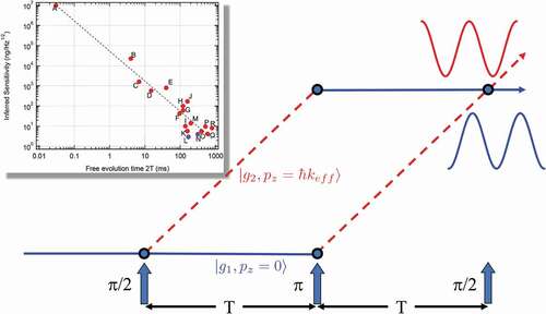
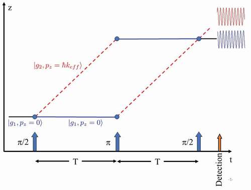
As previously mentioned, much of this article is focused on light-pulse atom interferometry. Although a variety of optical pulse types and sequences have been employed in light-pulse atom interferometers, here we focus on the most common Mach–Zehnder (or Kasevich–Chu [2]) interferometer type. This type of interferometer is often envisioned as depicted in Figure 1. In this atom interferometer design, a sequence of three optical pulses equally separated by time $T$ drives stimulated Raman transitions between internal atomic states $|g_1⟩\leftrightarrow |g_2⟩$ and imparts momentum $\Delta p=\pm \hslash k_{eff}$ in the process, where $k_{eff}$ is the effective 2-photon wave-vector. The optical pulses are labeled by the magnitude of the resulting Bloch vector rotation in radians, following the convention of nuclear magnetic resonance. A $\pi /2$ pulse creates a coherent superposition of a ground state $|g_1⟩$ with no momentum in the $z$-direction ($z$ being defined by the direction of the laser fields $k_1-k_2$) and another ground state $|g_2⟩$ with $\hslash (k_1-k_2)$ momentum in the $z$-direction. (For simplicity, the description above is in the inertial frame of reference of the atom.) As a result of the difference in momenta, the two trajectories diverge. After some free evolution time $T$, a $\pi$ pulse ‘flips’ the states and the resulting momentum kick to the atom redirects the trajectories toward each other. A final $\pi /2$ pulse a time $T$ later coherently recombines the two trajectories. As we will discuss here, for light-pulse atom interferometers, there is an additional contribution to the phase that arises from the interaction of the atoms with the laser pulses. The treatment below largely mirrors the treatment given in Schleich et al. [19] with the results that we highlight below also appearing in Storey and Cohen-Tannoudji [18].

Figure 1. Depiction of a light-pulse atom interferometer in real space. Atoms are either in a ground electronic state $|g_1⟩$ with momentum $p_z=0$ (blue solid lines) or in another ground electronic state $|g_2⟩$ with momentum $p_z=\hslash k_{eff}$. Direction of the arrows depicts the direction of the effective k vector.

Although the original Kasevich–Chu interferometer was realized using stimulated Raman transitions as the mechanism for momentum transfer, there are other methods to provide a momentum kick to the atoms such as Bragg transitions (see, e.g. [23–25].) and Bloch oscillations (see, e.g., [26,27].). We discuss some of these alternatives in the context of gravimetry in Section V B. Hereafter, we will refer to generic pulses that provide momentum to the atoms as Momentum Transfer Light Pulses (MTL pulses).

In Section II A, we reviewed the derivation of the result that the phase of the final wave function depends on the action taken over the classical path. For interfering paths $upper$ and $lower$, the phase difference due to this free propagation can be written as

(11) ${\varphi }_{prop}=\frac{1}{\hslash }\left(S_{cl}^{upper}-S_{cl}^{lower}\right)$(11)

where $S_{cl}$ is given by Equation (3)(3) $S_{\Gamma }={\int }_{t_a}^{t_b}dt\mathcal{L}[z(t),\dot{z}(t)].$(3) with the path $\Gamma$ chosen to be the classical path. For a free particle or an atom freely falling in a gravitational field, the action is the integral of kinetic energy minus the potential energy (0 and $mgz$ respectively). In the case of an atom in a rotating frame, the Lagrangian can be written in terms of the coordinates in the rotating frame (see Equation (23)(23) $=\frac{1}{2}m{v}^2+m\Omega \cdot (r\times v)+\frac{1}{2}m(\Omega \times r{)}^2$(23) ).

As an example, we consider the common light-pulse atom interferometer consisting of three Raman MTL pulses. The light–atom interaction may be modeled as an additional potential $V_{lp}$ given by [19]

(12) $V_{lp}=\sum _{j=0}^2\delta (t-jT)J_j(z)$(12)

where

(13) $J_j(z)\equiv \left\{\begin{array}{c}-\hslash [k_{eff}z+\varphi (jT)]\\ +\hslash [k_{eff}z+\varphi (jT)]\\ 0\end{array}\right.$(13)

where the minus sign corresponds to $|g_1⟩\to |g_2⟩$ transitions and the plus sign corresponds to $|g_2⟩\to |g_1⟩$ transitions. The zero indicates no interaction (at time $jT)$. Equation (13)(13) $J_j(z)\equiv \left\{\begin{array}{c}-\hslash [k_{eff}z+\varphi (jT)]\\ +\hslash [k_{eff}z+\varphi (jT)]\\ 0\end{array}\right.$(13) arises from the consideration of the time propagator for a two-level atom interacting with a single-mode field and describes the action of the atom beam splitters and mirrors. The integrals can be done trivially to find

(14a) $\frac{1}{\hslash }{\int }_{upper}dt{V}_{lp}=-[k_{eff}z(0)+\varphi (0)]+[k_{eff}{z}_{upper}(T)+\varphi (T)]$(14a)

(14b) $\frac{1}{\hslash }{\int }_{lower}dt{V}_{lp}=-[k_{eff}{z}_{lower}(T)+\varphi (T)]+[k_{eff}z(2T)+\varphi (2T)]$(14b)

Subtracting the lower arm from the upper arm (equivalent to traveling around the closed loop of the interferometer through the upper arm first and then the lower arm), we arrive at

(15a) ${\varphi }_{lp}=\frac{1}{\hslash }\left[{\int }_{upper}{V}_{lp}-{\int }_{lower}{V}_{lp}\right]-[{\varphi }_{pos}+{\varphi }_{phase}]$(15a)

where

(15b) ${\varphi }_{pos}=k_{eff}\left[z(2T)-z_{upper}(T)-z_{lower}(T)\right.\left.+z(0)\right]$(15b)

(15c) ${\varphi }_{phase}=\varphi (2T)-2\varphi (T)-\varphi (0)$(15c)

We find, then, that the interaction of the atoms with the laser pulses introduces two additional terms to the overall phase of the interferometer: the first one (${\varphi }_{pos})$ is the phase due to the position of the atoms at the time of the laser pulses and the second (${\varphi }_{phase}$) is the difference in phases of the laser at the time of the pulses, which accounts for changes due to phase fluctuations or intentional chirping of the laser frequency.

Finally, in addition to the phases calculated above, a third contribution appears in the phase of light-pulse atom interferometers: it is not always true that the classical paths terminating in a final point ($z_b,t_b$) originate at the same point ($z_0$, $t_a$). This phase term becomes nonzero in the case of gravity gradients, rotations, or unequal timing between MTL pulses. The phase due to this mismatch in classical origins of interfering paths is [28]

(16) ${\varphi }_{split}=\frac{p_0}{\hslash }(z_0^{upper}-z_0^{lower}).$(16)

The total phase of a light-pulse atom interferometer can then be written as

(17) $\Phi ={\varphi }_{prop}+{\varphi }_{lp}+{\varphi }_{split}$(17)

where ${\varphi }_{prop}$, ${\varphi }_{lp}$, and ${\varphi }_{split}$ are as defined above.

For many purposes, it is sufficient to take the classical limit $\hslash /m\to 0$, in which the spatial separation between the interfering atomic trajectories is eliminated and all interferometer phase arises from ${\varphi }_{lp}$. In this limit, the simple formula

(18) ${\Phi }_{class}=k_{eff}\left[z(2T)-2z(T)+z(0)\right]-{\varphi }_{phase}$(18)

is obtained.

1. A light-pulse atom interferometer gravimeter

We now apply the results of Section II B to the general case of an atom interferometer operating without rotation in a uniform and constant gravitational field with acceleration $-g$. Following a straightforward application of Newtonian mechanics, the terms of ${\varphi }_{pos}$ are given by

(19a) $z(2T)=\frac{\hslash k_{eff}}{m}T-2g{T}^2$(19a)

(19b) $z_{upper}(T)=\frac{\hslash k_{eff}}{m}T-\frac{1}{2}g{T}^2$(19b)

(19c) $z_{lower}(T)=-\frac{1}{2}g{T}^2$(19c)

(19d) $z(0)=0$(19d)

and ${\varphi }_{prop}={\varphi }_{split}=0$. We choose for this example ${\varphi }_{phase}=0$ (although this is not a good assumption for practical gravimeters as we discuss in V B) and generalize to three dimensions, obtaining

(20) $\Phi =k_{eff}\cdot g{T}^2$(20)

in agreement with ${\Phi }_{class}$. Deviations from this agreement will be found due to the introduction of gravity gradients, as we discuss in Section V B.

2. A light-pulse atom interferometer gyroscope

Light-pulse atom interferometry under constant rotation is commonly treated in the rotating frame of reference, although analysis in the inertial frame will, of course, obtain the same result. We begin by considering an inertial frame ${\mathcal{R}}^{\prime }$ (with coordinates $x^{\prime },y^{\prime },z^{\prime }$) and a rotating frame $\mathcal{R}$ (with coordinates $x,y,z$). The Lagrangian in the inertial frame is simply

(21) $L^{\prime }(r^{\prime },v^{\prime })=\frac{1}{2}m(v^{\prime }{)}^2$(21)

The transformation for velocity between inertial and rotating frame is given by

(22) $v^{\prime }=v+\Omega \times r$(22)

Because of the invariance of the Lagrangian under point-transformations, we may write the Lagrangian using the rotating coordinates

$\mathcal{L}(r,v)={\mathcal{L}}^{\prime }(r^{\prime },v^{\prime })$

$=\frac{1}{2}m{\left(v+\Omega \times r\right)}^2$

(23) $=\frac{1}{2}m{v}^2+m\Omega \cdot (r\times v)+\frac{1}{2}m(\Omega \times r{)}^2$(23)

From Lagrangian dynamics, we know that the momentum is given by

(24) $p=\frac{\partial \mathcal{L}}{\partial v}=mv+m\Omega \times r$(24)

A particularly intuitive expression is obtained for the propagation phase to first order in $\Omega$:

(25) $\begin{array}{cc}{\varphi }_{prop}& =\frac{m}{\hslash }\Omega \cdot {\int }_{t_a}^{t_b}dt\left[r(t)\times v(t)\right]\\ \hspace{0.17em}& =2\frac{m}{\hslash }\Omega \cdot A\end{array}$(25)

where $\mathcal{A}$ is the area (a vector) enclosed by the interferometer. In this approximation, then, the familiar Sagnac expression for the phase of an interferometric gyroscope is recovered [29].

In the light-pulse atom gyroscope, as in the gravimeter described above, the phase contains the contributions shown in Equation (17)(17) $\Phi ={\varphi }_{prop}+{\varphi }_{lp}+{\varphi }_{split}$(17) . In the three-pulse Mach–Zehnder configuration, the phase of a light-pulse atom interferometer at constant rotation rate $\Omega$, under constant acceleration $a$ with initial atomic velocity $v$ at location $R$ is (to second order in $|\Omega |$ and $T$) [30]:

(26) $\Phi =T^2{k}_{eff}\cdot \left(a-2\Omega \times v-\Omega \times \left(\Omega \times R\right)\right)$(26)

This expression gives rise to a simple interpretation of light-pulse atom interferometer phase in light of Equation 20(20) $\Phi =k_{eff}\cdot g{T}^2$(20) : the atom interferometer acts as an accelerometer that, in a rotating frame of reference, measures the sum of linear acceleration, Coriolis, and centrifugal accelerations. A common technique to differentiate phase due to rotation from phase due to acceleration is the measurement of two interfering paths with opposite values of $v$. By taking the sum and difference of the two measured phases, the rotation rate and acceleration may be inferred separately [31–33].

While this simple low-order light-pulse atom interferometer phase in Equation (26)(26) $\Phi =T^2{k}_{eff}\cdot \left(a-2\Omega \times v-\Omega \times \left(\Omega \times R\right)\right)$(26) is pedagogically valuable, the inclusion of higher-order terms is important for practical inertial sensing applications such as navigation. An analysis of light-pulse atom interferometry [30] discusses closed-form analytic expressions for shifts in accelerometer, gyroscope, optical clock and photon recoil measurement configurations. The analysis includes Coriolis, centrifugal, gravitational, and gravity gradient-induced forces. Calculations of effects out to fourth power of the time between pulses is given in Dubetsky and Kasevich [34].

C. Sensitivity of light-pulse atom interferometers

Based on the phases calculated above, simple expressions for sensitivity to accelerations and rotations in the presence of noise can be written. The single-shot acceleration noise of the atom accelerometer measurement is

(27) $\delta a=\frac{\delta {\Phi }_m}{k_{eff}{T}^2}.$(27)

Similarly, the single-shot rotation rate noise of a dual atom interferometer gyroscope is

(28) $\delta \Omega =\frac{\delta {\Phi }_m}{2\sqrt{2}{k}_{eff}v{T}^2}$(28)

In each case, $\delta {\Phi }_m$ is the noise in the measured phase of one atom interferometer. For the dual-atom gyroscope, it is the uncorrelated noise (added in quadrature) that does not cancel in the subtraction of measured atom interferometer phases.

For random, normally distributed $\delta {\Phi }_m$ with standard deviation ${\sigma }_{{\Phi }_m}$, these acceleration and rotation noise expressions may be easily translated into the inertially relevant sensitivities velocity random walk (VRW) and angle random walk (ARW) by replacing $\delta {\Phi }_m$ with the spectral density of noise in the phase measurement, $s_{{\Phi }_m}={\sigma }_{{\Phi }_m}\sqrt{t_{rep}}$ where $t_{rep}$ is the sensor measurement repetition time. We further discuss the effects of VRW and ARW in a navigation context in Section III. The contributions to $\delta {\Phi }_m$ include a myriad of factors including optical path noise, oscillator phase noise, laser frequency and intensity noise, differential laser phase noise, probe frequency and intensity noise, photon shot noise, and atomic quantum projection noise. Various studies have examined the major atom interferometer noise sources in detail [28,35,36], and we discuss the contribution of phase noise in Section IV B.

For atom interferometers measuring an ensemble of independent atoms, the fundamental limit to measurement sensitivity is due to quantum projection noise (QPN) [37]. This is straightforwardly estimated using a two-level atom model. For $N_a$ independent two-level atoms with states $|g_1⟩,|g_2⟩$ having population $p_1,p_2$, the measurement of total population in $|g_2⟩$ has mean $N_a{p}_2$ and variance ${\sigma }_2^2=N_a{p}_2(1-p_2)$. For each atom under ideal unitary evolution, $p_2=\frac{1}{2}(1+cos\Phi )$, and so

(29) ${\sigma }_{{\Phi }_{QPN}}=\frac{d\Phi }{d(N_a{p}_2)}{\sigma }_2=\frac{1}{\sqrt{N_a}}$(29)

This formula is independent of $\Phi$ for pure quantum projection noise. However, with the inclusion of technical noise sources, it becomes preferred to operate at the point of maximum slope of the atomic population versus phase. Modifications of this formula to account for inhomogeneous atomic position and velocity distribution, laser beam profile, spontaneous emission, decoherence, and other experimental details may derive a QPN limit for a particular sensor design. A density matrix formalism is typically useful in such ensemble noise analysis.

III. Navigation model

Navigation is a common motivation for atom interferometer development. For practical application of atom interferometry to inertial navigation, it is important to understand the performance metrics of atom interferometers in relation to the figures of merit for navigation. Briefly, this section will describe key performance parameters for inertial navigation, and outline a model for navigation performance based on those parameters to clarify their importance on different timescales. This model largely follows the work of Titterton and Weston [38].

An inertial navigation system typically comprises a three-axis accelerometer and a three-axis gyroscope, which detect the local motion of a platform relative to a constant velocity inertial frame of reference in flat Euclidean space. Data points are taken with a finite measurement bandwidth and an algorithm integrates these data points over time. The measurements of acceleration from the inertial frame are integrated twice to determine a new velocity and position, respectively. The measurements of rotation rate from the gyroscope must be integrated once to determine a new angle or heading and then this modifies the measured acceleration before being integrated twice.

The gyroscope measurements are therefore integrated three times compared to the accelerometer’s two integrals before a position estimate is made. This fact tends to increase the consequences of gyroscope measurement errors over accelerometer errors. Suppose there exists a systematic bias error (i.e. an inaccuracy) $B_a$ in an accelerometer. This will cause a position error $\delta x$ that grows quadratically in time: $\delta x\propto B_a{t}_{nav}^2$, where $t_{nav}$ is the time navigating since the last definitive position fix. Similarly, a rotation bias will cause a position error that grows with $t_{nav}^3$. This scaling is only true for navigation with respect to a flat, Euclidean inertial frame. On a spherical Earth, this scaling is valid at short timescales. Over longer times, Earth-frame navigation error accumulation is slower and is analyzed below.

Gyroscope measurements suffer from an additional complication due to the noncommutivity of rotations about different axes. If, during a single measurement interval, rotations about two or more axes occur in sequence, the gyroscope will record the same values regardless of order, but the true heading could depend on the order of those rotations. This ambiguity causes aliasing-like errors known as coning, sculling and scrolling, which are related to precession of the angular momentum, attitude or velocity vectors [39]. It is important for a gyroscope to make high-bandwidth measurements, which is a disadvantage for many atom interferometers as we mention in Section IV B. This fact led DARPA to fund the Chip-Scale Combinatorial Atomic Navigator (C-SCAN) [40] program to develop combinations of atom interferometers and higher measurement bandwidth sensors.

The estimation algorithm is commonly a Kalman filter, an analysis of which is well beyond the scope of this article. However, we can use some analytic approximations to demonstrate important trends. The accelerometer (gyroscope) can be modeled as generating a signal $S_a$ ($S_{\Omega }$) that is linearly dependent on the acceleration $a$ (rotation, $\Omega$), with a scale factor $F$ such that $S_a=F_{a}a$ ($S_{\Omega }=F_{\Omega }\Omega$). At zero acceleration or rotation, the output signal should be dominated by self-noise which can be characterized by the Allan deviation in the time domain [41]. The Allan deviation is the square root of the Allan variance, a two-sample variance revealing the contributions of noise sources to stability. The Allan deviation is particularly natural for atom interferometers that make measurements at finite times rather than continuously with some bandwidth.

Here, we consider three terms of a power law expansion of the Allan deviation of acceleration ${\sigma }_a(\tau )$ and rotation rate ${\sigma }_{\Omega }(\tau )$ in the measurement sample time $\tau$:

(30) $\begin{array}{cc}{\sigma }_a(\tau )& =VRW/\sqrt{\tau }+a_0+a_{RW}\sqrt{\tau }\\ {\sigma }_{\Omega }(\tau )& =ARW/\sqrt{\tau }+{\Omega }_0+{\Omega }_{RW}\sqrt{\tau }\end{array}$(30)

In each expression, the first term describes the Gaussian noise present in the measurement of $a$ and $\Omega$ respectively, with a coefficient called velocity random walk (VRW) or angle random walk (ARW). In the Allan deviation, this noise results in $1/\sqrt{\tau }$ dependence. The second term in the power law expansions of ${\sigma }_a$ and ${\sigma }_{\Omega }$ represents flicker or ‘bias’ noise present in the measurement and is a constant in $\tau$. Bias noise, a stochastic process that prevents one from averaging to arbitrary low statistical uncertainty, is not to be confused with bias errors, a systematic uncertainty that reduces measurement accuracy. The next terms in the Allan deviation power law expansion shown in Equation (30)(30) $\begin{array}{cc}{\sigma }_a(\tau )& =VRW/\sqrt{\tau }+a_0+a_{RW}\sqrt{\tau }\\ {\sigma }_{\Omega }(\tau )& =ARW/\sqrt{\tau }+{\Omega }_0+{\Omega }_{RW}\sqrt{\tau }\end{array}$(30) , are random or bias walk of acceleration or rotation rate, $a_{RW}$ and ${\Omega }_{RW}$, growing with $\sqrt{\tau }$. At short times, it is often possible to see Allan deviation decrease as $1/\tau$; this often arises from limited-bandwidth non-fundamental noise such as electronic noise. Not shown in Equation (30)(30) $\begin{array}{cc}{\sigma }_a(\tau )& =VRW/\sqrt{\tau }+a_0+a_{RW}\sqrt{\tau }\\ {\sigma }_{\Omega }(\tau )& =ARW/\sqrt{\tau }+{\Omega }_0+{\Omega }_{RW}\sqrt{\tau }\end{array}$(30) , there can also be bias drift – also known as bias run – which grows linearly with $\tau$. No fundamental physics source has been identified that creates bias walk or drift noise in light-pulse atom interferometers within the measurement capability of current atom interferometers. This is not true in mechanical or optical systems where thermal effects are known to cause such bias-walk and drift.

Briefly, we also discuss the term ‘resolution,’ which is a commonly reported quantity in laboratory evaluation of inertial sensors. Typically, resolution refers to the ability of a measurement to distinguish two values from each other, one of which may be zero, in which case resolution refers to the minimum detectable quantity that can be measured. In a static measurement, meaning that the quantity to be measured is not changing in time, then the resolution would likely be set by the minimum of the Allan deviation curve. This minimum could be determined by the bias noise terms ($a_0$ or ${\Omega }_0$) or by the combination of bias walk coefficient ($a_{RW}$ or ${\Omega }_{RW}$) with short-term stability (VRW or ARW). For example, one might attempt to measure the acceleration due to Earth’s gravity with a static atom interferometer after accounting for tidal effects. However, if the quantity to be measured is dynamic in time, then resolution will likely be limited by the short-term stability in combination with a measurement time that depends on the rate of fluctuations in the measured quantity. This latter case is typically the relevant case for navigation, since the platform motion varies on timescales much faster than the timescale for which bias noise is a factor. For this reason, resolution can be a confusing quantity to use in navigation applications and will not be used further in this navigation analysis.

In the presence of non-zero acceleration and rotation, one must also consider the case that the scale factor $F$ is not perfectly known or constant. Scale factor instability occurs when a scale factor changes in time. A scale factor that changes with increasing inertial input is known as a scale factor non-linearity. Consider a rotation measurement with a combination of scale factor instability and measurement noise: then the sensor variance becomes ${\sigma }_{S_{\Omega }}^2=F_{\Omega }^2{\sigma }_{\Omega }^2+{\Omega }^2{\sigma }_{F_{\Omega }}^2=F_{\Omega }^2{\sigma }_{\Omega }^2+S_{\Omega }^2({\sigma }_{F_{\Omega }}^2/F_{\Omega }^2)$. The term ${\sigma }_{F_{\Omega }}/F_{\Omega }=SFS$ is the scale factor stability (SFS), which is unitless. One can also see that the sensor noise will be dominated by measurement noise at very low signal (inertial input) and dominated by SFS noise at large input signal. This fact leads many high-performance gyroscopes to be rotationally stabilized inside of gimbals such that the rotation input is always near zero and thus the SFS and scale factor non-linearity have negligible impact. Any estimation algorithm must take SFS and nonlinearites into consideration.

We now move on to navigation in the rotating, non-inertial, spherical reference frame of the Earth. The navigation estimation algorithm must project the position estimate from a flat Cartesian inertial frame of the platform onto Earth frame including its rotation, curvature, and gravity field. The projection can take advantage of knowledge of the Earth’s curvature and rotation rate to partially remove measurement biases. For example, on timescales longer than 24 h, the gyroscope can measure Earth rate and thus any bias error. The curvature term is more subtle and relies on using the accelerometer and gyroscope together. To understand, imagine a platform initially moving due East at low altitude over the equator at constant speed that also attempts to make its accelerometer and gyroscope read zero. To accomplish this feat, it must accelerate so as to counteract gravity and therefore be in free-fall. The hypothetical platform must actually be in orbit and its orbital period is the Schuler period $T_S=2\pi \sqrt{R_E/g}\approx 84$ min, where $R_E$ is the Earth radius. On this hypothetical orbiting platform, the accelerometer measurement could have a bias error, but on one side of Earth this will be biased in the opposite direction as on the other side of the Earth. These directions are relative to the local platform inertial frame and so the vector bias will tend to rotate at the Schuler period. In a real platform, gravity is computationally removed from the accelerometer measurement in order to isolate platform motion. The estimation algorithm will encounter an oscillation at the Schuler period during this process because an accelerometer bias will manifest as an apparent rotation of the gravity vector that will not agree with the gyroscope reading. This observation can be used to remove accelerometer and gyroscope biases on times scales longer than about 1.5 h. Inertial navigation position error thus accumulates differently according to which timescale is considered: $t_{nav}\stackrel{<}{\sim \phantom{{ }_x}}{T}_S$, $T_S\stackrel{<}{\sim \phantom{{ }_x}}{t}_{nav}\stackrel{<}{\sim \phantom{{ }_x}}{T}_E$ and $t_{nav}\stackrel{>}{\sim \phantom{{ }_x}}{T}_E$, where $T_E$ is the Earth rotational period.

For the fastest timescale, $t_{nav}<T_S$, position errors accumulate in time as in flat Euclidean space: as $B_{\Omega }{t}_{nav}^3$ and $B_a{t}_{nav}^2$ for the gyroscope and accelerometer biases $B_{\Omega }$ and $B_a$ respectively. For the timescales less than Earth period, $t_{nav}<T_E$, from Titterton and Weston [38], position errors accumulate as

(31) ${\sigma }_x=B_{\Omega }R\left(t-\frac{sin{\omega }_S{t}_{nav}}{{\omega }_S}\right)+B_a\left(\frac{1-cos{\omega }_S{t}_{nav}}{{\omega }_S^2}\right)$(31)

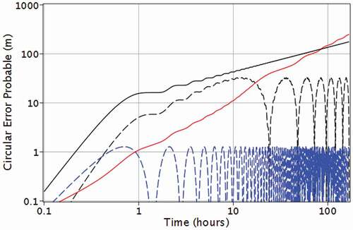
where ${\omega }_S=2\pi /T_S$ and $R$ is the radius of curvature, typically the radius of the Earth. The longer-timescale error accumulation is complicated by additional oscillation terms at Earth rate and its projection onto the gravity vector depends on latitude. Figure 2 shows the relative contributions to horizontal error often referred to as circular error probable (CEP) for a hypothetical case. It is on a log plot so one can clearly see the the relative contributions on the three timescales described.

Figure 2. The contribution to horizontal navigation position error due to ARW of 100 ${\mu }^{\circ }/\sqrt{h}$ or 29 nrad/$\sqrt{s}$ (solid black), gyro bias about a horizontal axis (black dash) and the vertical axis (red solid) of 50 ${\mu }^{\circ }/h$ (0.24 nrad/s) and accelerometer bias (blue dash) of 100 μg. Note the Schuler oscillations at 84 min and the Earth rate oscillation at 34 h which is the vertical projection of Earth rate at 45 degree latitude, the latitude used in this data.

Accurately modeling an inertial navigation system would require more terms based on initial alignment, environmental contributions, sampling errors (such as coning error), scale factor errors, axis cross-coupling (for not perfectly orthogonal systems), as well as potentially engineering methods to reduce biases such as purposely oscillating or periodically flipping a gyroscope. (The reader is advised to read reference [38] for details).

When determining the acceleration of a platform, one must subtract the acceleration due to gravity. Special relativity guarantees that one cannot separate the two with an acceleration measurement alone. This fact will lead to unconstrained errors in altitude. Fortunately, a simple altimeter or depth sensor can prevent this.

Worse, gravity is not a constant across the Earth. Typically, one must use precise gravity maps for this purpose [42]. These maps are made with the best portable accelerometers; however, if atom interferometers are made more sensitive than the previous state of the art and are to be used for navigation, better maps will be required in order to take advantage. There is another possibility: one can use a gravity gradiometer to isolate the local gravity value from the acceleration value. In this way, a future inertial navigation system with gravity gradiometers could simultaneously extend navigation capability while also developing new gravity maps over time.

IV. Challenges and solutions for practical implementation

For applications in the field, and particularly for inertial navigation on moving platforms, a number of goals must be met by atom interferometers. The obvious metrological performance metrics such as sensitivity, accuracy, and stability have been the highlighted outcomes of many laboratory demonstrations over the years. Other practical goals in fielding atom interferometers include reduced size, weight, and power consumption compatible with platforms of interest; high reliability; manufacturability; and low cost. In this section, we focus on four key areas: dynamic range, bandwidth, performance under platform motion, and size. These areas are of particular interest in determining the promise of the technology because they are driven largely by basic sensor architecture and design parameters. They are not fundamentally determined by the technological details of supporting subsystems. These technological areas, while important, are complementary to the issues presented here. Atom interferometer supporting technologies are treated in some detail in the review article of Geiger et al. [10].

A. Dynamic range

In sensing contexts, dynamic range (DR) refers to the ratio of the largest to the smallest signal that can be measured. In typical atom interferometer inertial sensors, the dynamic quantity of interest is proportional to the interferometer phase $\Phi$. However, the directly measured quantity is state population, which is a sinusoidal function of phase, resulting in ambiguity in determining $\Phi$. Naively, then, the largest unambiguously measurable phase in a single measurement is $\pm \pi /2$, while the smallest measurable phase is $\delta {\Phi }_m$, the measured phase noise. The dynamic range is then $DR=\frac{\pi }{2\delta {\Phi }_m}$, which, for commonly achieved values of sensor phase noise, is frequently in the range $10<DR<{10}^4$ in a 1-s measurement time. Alternatively, the term ‘dynamic range’ is sometimes used instead to simply refer to the largest unambiguously measurable dynamic quantity [43]. For a light-pulse atom accelerometer with $\Phi =k_{eff}\cdot a{T}^2$, this maximum range of unambiguous measurement is

(32) $a_{max}=\pm \frac{\pi }{2|k_{eff}|T^2}.$(32)

For example, for a standard two-photon Raman atom interferometer with $T=50$ ms in ⁸⁷Rb, this measurable range of accelerations in open loop is $\pm 8$ μg. This naive mode of operation with very low dynamic range, while pedagogically useful, is impractical for most applications.

Achieving dynamic range sufficient to ensure compatibility with desired operational conditions is a major goal in practical atom interferometer design. Numerous methods of increasing dynamic range have been developed. The introduction of a closed-loop mode of operation can increase dynamic range enormously. For closed-loop operation, the phase or frequency of the driving laser beams is servoed so that the total interferometer phase is always near to zero. In gravimeters, for example, this closed-loop operation implies a chirp in the MTL frequency difference that cancels the Doppler shift due to gravitational acceleration [28]. In gyroscopes, equal and opposite frequency shifts proportional to rotation rate are applied to the first and third MTL frequency differences, such that the sum of the dynamic phase and the laser phase is nearly zero [36,44]. In either case, operation at the point of maximum sensitivity and linearity occurs so long as the appropriate frequency and phase corrections can be estimated, subject to further limitations discussed in Section IV C. Such closed-loop operation requires a method of estimating the necessary frequency and phase to be applied to the laser pulses to reach the zero-phase point of operation. In gravimeters, simple knowledge of the approximate value of the local acceleration due to gravity may be sufficient. This may be obtained from the atom interferometer itself by operating over a range of values of $T$ [45]. Once a point of operation within $\pi /2$ of the zero-phase point is reached, the atomic signal may then be used to provide a servo error signal and track changes in input signal to increase dynamic range. A novel ‘composite-fringe’ technique that combined measurements at multiple values of $T$ was demonstrated to increase dynamic range by two orders of magnitude even for time-varying dynamics [46].

When high-frequency dynamics cause the interferometer phase to change by a significant fraction of $\pi$ at a rate faster than the atom interferometer measurement bandwidth, a servo based on the measured atomic signal alone is not sufficient to maintain dynamic range. In nearly static applications, low-amplitude, high-frequency dynamics may be reduced through the use of active or passive vibration isolation platforms [47–50]. In applications where high-frequency dynamics must be measured, hybridization of the atom interferometer with a high-bandwidth auxiliary sensor can increase dynamic range. Such fusion may take multiple forms: in some work, the co-sensor data is used to compute phase corrections to the atom interferometer, which are then applied to the interferometer sequence via the two-photon optical frequency and phase difference [51,52]. In other work, data captured from the co-sensor is fused with the output of the atom interferometer after both are captured by estimation techniques such as Kalman filters [53,54]. The latter set of techniques may be thought of as using the atom interferometer’s superior bias drift and scale factor stability to reduce the low-frequency drift of the high-bandwidth auxiliary sensor. These sensor hybridization techniques have the advantage of not only improving dynamic range but also addressing the related challenges of bandwidth and dead time, as we discuss in the next section.

B. Bandwidth, dead time, and aliasing

Atom interferometers, particularly those based on periodically laser-cooled ensembles of atoms, commonly suffer from the interrelated challenges of low measurement bandwidth and dead time. This stands in contrast to conventional mechanical or optical inertial measurement units, for which measurement rate may far surpass 100 Hz and dead time is negligible. (In gravimetry, on the other hand, atom interferometer bandwidth is often higher than that of conventional high-accuracy absolute gravimeters [55].) For a periodic light-pulse atom interferometer measurement at repetition period $t_{rep}>2T$, the Nyquist-limited measurement bandwidth is $f_{BW}=f_{rep}/2=(2t_{rep}{)}^{-1}$. In most cold-atom interferometer experiments, the repetition time is determined by the time $t_{load}$ needed for sufficient atom numbers to be trapped, cooled, and state-prepared, as well as the actual interferometer time $2T$ and detection duration $t_{det}$, so that $t_{rep}>t_{load}+2T+t_{det}$. The ‘dead time’ of the sensor, during which no inertial measurement is being made, is therefore $t_{rep}-2T$. Commonly, in laboratory pulsed atom interferometers based on magneto-optical trap (MOT) and atomic fountain configurations, 0.1 s $<t_{rep}<$ 2 s, although exceptions exist on either extreme as discussed in Section 5. Advanced cooling techniques, such as evaporative cooling to degeneracy, increase the value of $t_{rep}$, with rapid chip-based evaporation techniques typically requiring $t_{load}>1$ s [56].

In the presence of signals and noise at frequencies higher than $f_{BW}$ in a pulsed atom interferometer, aliasing can occur. This is closely related to the Dick effect in pulsed atomic clocks, whereby local oscillator phase noise degrades the frequency stability of the clock [57]. In inertial measurement, aliasing of noise sources such as vibration leads to a degradation of sensitivity. In navigation applications, error in the response to aliased dynamics leads to error in the navigation solution [58]. The impact of aliasing of a variety of noise sources in atom interferometers was calculated in depth in Refs [59] and [36]. A simple expression for the Allan variance of the measured interferometer phase for a standard 3-Raman pulse interferometer due to aliased phase noise is achieved in the limit of large averaging window $\tau$ [59]:

(33) ${\sigma }_{{\Phi }_m}^2(\tau )=\frac{1}{\tau }\sum _{n=1}^{\infty }|H(2\pi n{f}_{rep}){|}^2{S}_{\varphi }(2\pi n{f}_{rep})$(33)

where $S_{\varphi }$ is the power spectral density of phase noise and $H(\omega )$ is the transfer function of the atom interferometer

(34) $\begin{array}{cc}H(\omega )=& \frac{4i{\omega }_R\omega }{{\omega }^2-{\omega }_R^2}sin\left(\frac{\omega (T+2{\tau }_R)}{2}\right)\\ \hspace{0.17em}& \times \left(cos\left(\frac{\omega (T+2{\tau }_R)}{2}\right)+\frac{{\omega }_R}{\omega }sin\left(\frac{\omega T}{2}\right)\right).\end{array}$(34)

Here, ${\tau }_R$ is the Raman pulse duration and ${\omega }_R$ is the Rabi frequency of the Raman transition. This implies that phase noise at multiples of the repetition frequency degrades interferometer sensitivity. In Cheinet et al. [59], $H(\omega )$ is directly measured in a Doppler-insensitive three-pulse atom interferometer configuration.

To eliminate dead time, two primary solutions have been developed. First is the selection of an atom interferometer timing sequence that eliminates dead time. Continuous operation, as in thermal beam atomic gyroscopes, effectively eliminates aliasing due to dead time [36,60–62]. Truly continuous operation typically requires operation in the spatial domain, wherein the scale factor of the interferometer is determined by the spatial separation of the MTL beams rather than the timing of laser pulses.

Alternatively, pulsed operation in an interleaved ‘zero-dead-time’ mode of operation, with atom interferometer repetition time $t_{rep}\approx T$, likewise eliminates errors due to dead time. This follows from the fact that the weighting function $H(\omega$) has zeros at $\omega =\frac{2\pi n}{T+2{\tau }_R}$ for integer $n\ge 0$. This method of operation was first published in a patent [63] and was first demonstrated by AOSense, Inc., in a cold-atom accelerometer/gyroscope sensor in the DARPA PINS II program [64]. Zero-dead-time operation was also applied to fountain clocks [65] and was experimentally shown to result in improved Allan deviation in atomic gyroscopes [66,67].

The second demonstrated method of eliminating dead time arises from hybridization with conventional cosensors as discussed in the preceding section [53,54]. The fusion of periodic atom interferometer signals with continuous, high-bandwidth conventional sensor outputs provides an output without dead time. The disadvantage of this approach is that the short-term sensitivity (angle random walk or velocity random walk) of the combined sensor is limited by the conventional sensor, even if the atom interferometer produces superior short-term sensitivity on its own.

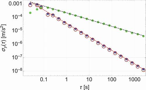
Examples of the effect of aliasing on atom accelerometer Allan deviation curves under various assumptions of sensor timing and vibration spectrum are shown in Figure 3. There we evaluate the Allan deviation of a light-pulse atom accelerometer in response to limited-bandwidth uncorrelated vibration noise, under three different conditions: vibration noise entirely at frequencies below $f_{BW}$; vibration noise centered around $f_{rep}$ leading to aliasing; and a zero-dead-time $t_{rep}=T$ configuration that mitigates aliasing. This figure illustrates the fact that aliasing of high-bandwidth noise leads to degraded stability even at long measurement times, which can be mitigated by continuous or zero-dead-time operation, or by operation at sufficiently high rate to capture the noise.

Figure 3. Modeled Allan deviation of light-pulse atom interferometer accelerometer response to vibrations under three different conditions. All other noise sources are ignored for the purpose of illustration. Blue dots: Atom interferometer without aliasing. $T=10$ ms, $t_{rep}=25$ ms, Nyquist frequency is $f_{BW}=20$ Hz. Input vibration has rms acceleration 1 mm/s² and flat acceleration power spectrum from 5 to 15 Hz (0 at all other frequencies), so that it lies entirely within the measurement bandwidth of the sensor. The Allan deviation integrates down as ${\tau }^{-1}$ (red dashed line). Green dots: Atom interferometer exhibiting aliasing. $T=10$ ms, $t_{rep}=25$ ms, Nyquist frequency is $f_{BW}=20$ Hz. Input vibration has rms acceleration 1 mm/s² and flat acceleration power spectrum from 35 to 45 Hz (0 at all other frequencies). The Allan deviation integrates down as ${\tau }^{-1/2}$ (dashed black line). Red open circles: Zero-dead-time configuration to eliminate aliasing. $T=t_{rep}=25$ ms, so that Nyquist frequency remains $f_{BW}=20$ Hz. Input vibration power spectrum is the sum of that on the other two plots, with rms acceleration 1.4 mm/s²: flat from 5 to 15 Hz and from 35 to 45 Hz (0 at all other frequencies). The Allan deviation integrates down as ${\tau }^{-1}$.

C. Dynamic contrast loss and cross-axis coupling

In Section IV A, we discussed dynamic range in the sense of the maximum and minimum measurable inertial signals along the atom interferometer’s nominal axis of rotation or acceleration sensitivity. Light-pulse atom interferometer sensitivity and accuracy can be further degraded by motion in the sense of systematic error and reduced interference contrast that occur as a result of accelerations and rotations in three dimensions, and not solely along the sensor’s nominal axis of sensitivity. Both phase errors and contrast loss can be described in terms of the atom interferometer phases that develop in response to motion. Atom interferometer phase contributions due to numerous sources have been calculated using the Feynman path integral formulation of atom interferometry [30]. For example, under a rotation rate $\Omega$, an atom with velocity $v_a$ develops a Coriolis phase shift [20,68]

(35) ${\varphi }_{Cor}=2(v_a\times \Omega )\cdot k_{eff}{T}^2$(35)

This phase shift constitutes both a systematic phase error for a gravimeter under rotation in the presence of uncharacterized mean atomic velocity and also a source of reduced contrast due to the nonzero temperature of the atomic ensemble.

Integration of motion-induced phases over the classical atomic position and velocity distribution allows the estimation of the degradation of interferometer’s normalized fringe amplitude, or fringe contrast, in the presence of dynamics. For example, integration of Coriolis phase over a Gaussian 1D atomic velocity distribution with velocity standard deviation ${\sigma }_v$ reveals a reduction in the fringe contrast $C$ due to rotation [62]:

(36) $C\propto exp(-2k_{eff}^2{T}^4{\Omega }^2{\sigma }_v^2).$(36)

In this case ${\sigma }_v$ is the velocity width along the axis perpendicular to $\Omega$ and $k_{eff}$. Similar to the Coriolis-induced contrast degradation, contrast loss also arises due to the centrifugal phase averaged over atomic position distribution. These contrast degradation effects arise in a treatment of atoms as classical, pointlike particles drawn from a distribution of classical positions and velocities. A quantum treatment of wavepacket evolution in atom interferometry reveals that rotation-induced contrast loss also occurs at the single-atom level [20]: under rotation, single-atom interference paths fail to close perfectly, resulting in contrast loss that depends upon the coherence length of the wavepacket.

In spatial-domain atom interferometers using continuous atom beams [9,60], the timing of MTL pulses is determined by their spatial arrangement combined with the atomic trajectory. Additional contrast loss mechanisms exist due to the dependence $T=L/|v_a|$, where $L$ is the separation between the MTL beams. The resulting inhomogeneity in scale factor due to the distribution of $v_a$ causes reduced contrast under acceleration and rotation. For spatial-domain atom gyroscopes using Raman pulses, closed-loop operation in which the Raman frequencies are adjusted to compensate for rotation and acceleration as described above greatly increases the size of the contrast envelope of the atom interferometer [32]. A second cause of contrast reduction in spatial-domain interferometers occurs due to acceleration along the atom beam propagation direction [62]. In this case, the two time separations between adjacent MTL pulses become unequal due to the changing atomic velocity in the frame of reference of the laser beams. The resulting loss of contrast depends upon the atomic temperature and acceleration [69,70].

As suggested by the expression for Coriolis-induced contrast loss above, it is generally true that reducing the interrogation time $T$ and reducing the velocity width ${\sigma }_v$ mitigate contrast loss and phase error due to dynamics. However, reduction in $T$ naturally comes at a cost in short-term sensitivity. We summarize these trade-offs in Figure 4 and Figure 5 for a light-pulse atom interferometer with fixed phase-noise density of $s_{{\Phi }_m}=1mrad/\sqrt{H}z$ . The contours in these figures are determined by solving for a maximum interrogation time $T_{max}$ consistent with an $exp(-2)$ contrast loss under rotation ${\Omega }_{max}$ in Equation (36)(36) $C\propto exp(-2k_{eff}^2{T}^4{\Omega }^2{\sigma }_v^2).$(36) and calculating static ARW and VRW. (The −2 exponent is arbitrarily chosen.) It should be noted that the choice of phase noise in the figures is arbitrary, and must be adjusted for each interferometer design. In this view, the absolute (for accelerometers, Figure 4) or the normalized (for gyroscopes, Figure 5) velocity width is a critical determinant of performance under rotation. Either cooling or velocity selection may reduce the velocity width of the atomic ensemble, but each method results in trade-offs in atomic flux, measurement rate, and sensor complexity. Expected operational conditions and the required inertial sensitivity in a particular application therefore have a substantial effect on the optimal value of $T$ and the extent of cooling or velocity selection to be employed.

Figure 4. Light-pulse atom interferometer acceleration measurement sensitivity (VRW) in ng/$\sqrt{Hz}$ versus designed maximum rotation rate ${\Omega }_{max}$ and 1D atomic velocity width ${\sigma }_v$, with white atom interferometer phase noise $s_{{\Phi }_m}=1$ mrad/$\sqrt{Hz}$. ${\Omega }_{max}$ is the rotation rate such that fringe contrast (see Equation (36)(36) $C\propto exp(-2k_{eff}^2{T}^4{\Omega }^2{\sigma }_v^2).$(36) ) is reduced by $exp(-2)$ due to the Coriolis effect. The VRW shown should be adjusted in proportion to the assumed phase noise.

Figure 5. Light-pulse atom interferometer gyroscope measurement sensitivity (ARW) in rad/$\sqrt{s}$ versus designed maximum rotation rate ${\Omega }_{max}$ and the ratio of 1D atomic velocity width ${\sigma }_v$ and mean atomic velocity $v$, with white atom interferometer phase noise $s_{{\Phi }_m}=1$ mrad/$\sqrt{Hz}$. ${\Omega }_{max}$ is the rotation rate such that fringe contrast (see Equation (36)(36) $C\propto exp(-2k_{eff}^2{T}^4{\Omega }^2{\sigma }_v^2).$(36) ) is reduced by $exp(-2)$ due to the Coriolis effect. The ARW shown should be adjusted in proportion to the assumed phase noise.

To combat phase error and fringe contrast loss due to rotation, a successful solution has been the actuation of MTL beam pointing. The goal is to maintain the parallelism of wavevectors of the MTL pulses making up each interferometer sequence in the freefall reference frame of the atoms, so that no perturbation of interferometer phase due to rotation occurs. This method was applied to eliminate phase shifts and contrast loss due to Earth rotation at Stanford [71] and subsequently at Berkeley [20] and Berlin [72]. These demonstrations of the actuation of MTL beam pointing have all taken place under conditions of constant and predictable sensor rotation rate. In demonstrations of atom interferometry on a moving vehicle with time-varying rotation rate, active gimbal stabilization of the entire sensor physics package has accomplished much the same goal [73,74].

Alternatively, spatially resolved measurement of atom interferometer phase can increase contrast under rotation by resolving rotation-induced phase shear [75–77]. A particular method of spatially resolved interferometry is point-source atom interferometry (PSAI) [22,78–81]. PSAI takes advantage of the linearity of Coriolis phase in the atomic velocity. In PSAI, during free evolution, the atomic ensemble is allowed to expand until the position of atoms in the plane perpendicular to the MTL beams is strongly correlated with initial atomic velocity. Spatially resolved measurement of the atomic population can then determine phase as a function of velocity, providing a measurement of rotation rate even in the case that multiple $2\pi$ phase wraps are present across the atomic ensemble, and also distinguishing such rotation from uniform acceleration. Such phase inhomogeneity would result in very low contrast with conventional, unresolved population detection integrated over the ensemble. Further, if imaging of atomic population occurs along the direction of MTL beam propagation, measurement of rotation rate along two axes simultaneously is enabled. While PSAI increases dynamic range by allowing the measurement of multiple-$2\pi$ phase excursions across the atom cloud, it does not indefinitely increase allowable rotation rates for two reasons: (1) single-atom loss of interference constrast as described in Lan et al. [20]; and (2) the finite initial size of the atom cloud blurs the interference fringes, resulting in a loss of visibility for sufficiently high spatial frequency [80]. A quantum mechanical treatment of point source interferometry is given in Li et al. [22]. We provide further examples of experimental demonstrations of PSAI in Section VI E.

D. Size

Technological limitations pose challenges in the size, weight, power consumption, and cost (SWaP-C) of atom interferometer-based sensors. The key subsystems include lasers; optical beamshaping, routing, frequency, and intensity control; electronic signal sources, timing, and data acquisition; magnetic field control including coils and shielding; and vacuum systems including enclosures, windows, and pumps. An overview of these subsystems is presented in Geiger et al. [10]. Apparatus to enable high-performance operation outside of the laboratory can also contribute strongly to SWaP-C. These can include vibration isolation as discussed in Section V B, temperature isolation and control, and gimbals in some applications. Engineering improvements to all of the above systems are likely to lead to more compact and fieldable atom-based inertial sensors.

In this section, we discuss more fundamental limitations to atom interferometer size based on the scale of the atomic trajectory. In most light-pulse atom interferometers, by design the atoms are in freefall during the interrogation time (with several exceptions as noted in Sections V B and VII). The fundamental lower bound on the size of a freefall atom interferometer is therefore determined by the ballistic motion of the atoms and depends on the dynamic environment. Under acceleration, the vacuum cell, MTL beam extents, and detection volume must, at a minimum, have spatial dimension large enough to account for the motion of atoms in freefall during the free-flight time $\ge 2T$. When the magnitude and direction of acceleration are approximately predictable, as in nearly static gravimetry applications, it is sufficient to extend the size of the apparatus only along the direction of acceleration, which is commonly also the direction of MTL beam propagation. However, for accelerations in arbitrary and varying directions, as in the case of strapdown inertial navigation, it becomes necessary to extend the apparatus size, including laser beam waist, in three dimensions. For some combinations of acceleration and $T$, this is likely to be impractical. These considerations are in addition to the issue of contrast loss under dynamics as described in Section IV C.

In Figures 6 and 7, we illustrate the basic relationship between trajectory size, atomic velocity, and platform acceleration for ⁸⁷Rb accelerometers and gyroscopes respectively. In Figure 6, the size is determined by the atoms’ ballistic flight under 1D acceleration $a$. The interrogation time $T$ is calculated based on size and $a$, and sensitivity is inferred by assuming a fixed phase noise of 1 mrad/$\sqrt{Hz}$. In Figure 7 the size is determined by the atoms’ ballistic flight following launch at velocity $v$. The interrogation time $T$ is calculated based on size and $v$, and sensitivity is inferred by assuming a fixed phase noise density of 1 mrad/$\sqrt{Hz}$. The choice of phase noise in these figures is arbitrary and should be scaled according to sensor design. In Section VI G, we expand upon this simple model of atom interferometer size and sensitivity.

Figure 6. Acceleration measurement sensitivity (VRW) [ng/$\sqrt{Hz}$] of a $2\hslash k$ ⁸⁷Rb Raman atom interferometer as a function of spatial dimension $d=2a{T}^2$ and applied acceleration $a$, in a dropped-atom configuration with white phase noise $s_{{\Phi }_m}=1$ mrad/$\sqrt{Hz}$. The spatial dimension shown may be the size along the Raman beam propagation direction in the case of measurement along a predictable acceleration axis (gravimetry) or it may be the transverse beam size in the case of unpredictable acceleration direction. The acceleration sensitivity (VRW) shown should be adjusted in proportion to the assumed phase noise.

Figure 7. Gyroscope measurement sensitivity (ARW) [rad/$\sqrt{s}$] of a $2\hslash k$ Raman ⁸⁷Rb atom interferometer as a function of spatial dimension $d=2vT$ and atomic velocity $v$, with white phase noise $s_{{\Phi }_m}=1$ mrad/$\sqrt{Hz}$. The spatial dimension shown is the size along the atom propagation direction ignoring the effect of accelerations, gravity, and rotations. The gyroscope sensitivity (ARW) shown should be adjusted in proportion to the assumed phase noise.

A number of improvements to the size of atom interferometer accelerometers and gyroscopes have been presented and discussed in greater detail elsewhere in this article. Elimination or modification of the ballistic trajectory of the atoms through trapping or momentum redirection can lead to substantial size reductions, as we discuss in Section VII. Increasing scale factor through large-momentum-transfer atom optics can potentially allow for a reduction in size without a concomitant degradation in performance as we discuss in Section V B.

Within the basic architecture of freefall light-pulse interferometry, reduction of the interrogation time $T$ has numerous benefits as we discuss above, including improvement of dynamic range, measurement bandwidth, fringe contrast under rotation and acceleration, and size. However, these improvements come at the cost of a reduction in scale factor and hence a reduction in sensitivity for a given phase measurement noise $s_{{\Phi }_m}$.

The reduction in inertial sensitivity resulting from operating at reduced $T$ can, in principle, be compensated by operating at high signal-to-noise ratio or by increasing the sensor scale factor by operating with increased momentum separation between the arms of the atom interferometer. For high-flux atom interferometers, technical noise sources are often dominant over quantum projection noise [35,45,51,67]. However, some experiments do approach the quantum projection noise limit [82,83]. Broadly speaking, in pulsed cold-atom interferometer experiments to date, measured phase noise is commonly in the range ${10}^{-3}$ rad/$\sqrt{Hz}$ $<s_{{\Phi }_m}<{10}^{-1}$ rad/$\sqrt{Hz}$ as may be inferred from the collection of experiments cited in Figure 9. If operation near the quantum projection noise limit can be routinely obtained, improvements upon this common behavior may be available. Using standard laser-cooling techniques, a cold-atom throughput of ${10}^9$ atoms/s or higher is feasible [84], resulting in a possible quantum projection noise limit of $s_{QPN}\le {10}^{-4}$ rad/$\sqrt{Hz}$. Using high-flux hot atom beam techniques, the quantum projection noise limit can be even lower due to the larger throughput of atoms despite typically lower contrast. An inferred phase noise of 60 μrad/$\sqrt{Hz}$ was obtained in the transversely cooled, fast Cs beam of the Yale gyroscope in Gustavson et al. [44]. This suggests that such low phase noise may be more generally achievable, and excellent inertial sensitivity may be obtained even at reduced values of $T$. The result would be reduced size and improved dynamic response compared with typical laboratory experiments.

V. Accelerometers and gravimeters

A. Accelerometer model

By far the most widely used sensor architecture for accelerometers based on atom interferometry is the Kasevich–Chu light-pulse atom interferometer using laser-cooled atoms interrogated by counterpropagating optical fields driving stimulated Raman transitions. Here, we provide an overview of the principles of operation and practical considerations for this sensor type. As we discuss below, numerous variations on this common architecture have been demonstrated including the use of Bragg transitions (in which the internal state of the atom is unchanged) rather than Raman transitions; the use of additional laser pulses to increase momentum separation between interferometer arms; the use of optical potentials to modify atomic trajectories; the use of narrow one-photon optical transitions rather than two-photon Raman transitions; and numerous variations in laser cooling and trapping techniques.

Gravimeters that accurately report the total local gravitational acceleration are described as absolute, while those that report differences or changes in gravitational acceleration are described as relative. Because of their inherent calibration based on accurately known time and optical wavelengths, light-pulse atom gravimeters are generally described as absolute gravimeters. A general review of atom-based gravimeters was published in 2008 [85].

As we discuss in Section II, the phase of an atom interferometer is most readily estimated using the Feynman path integral approach [18]. This is calculated in detail for the case of gravimeters (and, equivalently, accelerometers) based on the three-pulse Raman configuration in Peters et al. [28], and the calculation can be adapted to more general MTL pulses. In the presence of constant gravitational acceleration term $g_z$ and first spatial derivative ${\gamma }_{zz}$ of gravitational acceleration along the $z$ direction, the Lagrangian is

(37) $\mathcal{L}(z,\dot{z})=\frac{m{\dot{z}}^2}{2}-m{g}_{z}z+\frac{m{\gamma }_{zz}{z}^2}{2}$(37)

This Lagrangian may be used to calculate the classical atom trajectories and classical action, from which the total phase is computed. In many cases, it is most convenient to perform this calculation perturbatively. The resulting phase in a light-pulse atom interferometer, to first order in ${\gamma }_{zz}$, is

(38) $\Phi =k_{eff}{T}^2\left(g_z+{\gamma }_{zz}\left(\frac{7}{12}{g}_z{T}^2-v_{0}T-z_0\right)\right)$(38)

This equation is valid in the case of time-invariant gravity without rotations. As expected, gravity measurements made with identical atom interferometers separated by a baseline $L_z$ will differ in their gravity measurements by ${\gamma }_{zz}{L}_z$. It should be noted that gravity gradient has SI units of m/s²/m = s^–2, and a common unit is the Eötvös, E = 10^–9 s^–2. The vertical gravity gradient near the Earth’s surface is ${\gamma }_{zz}\approx 3080$ E. The inclusion of rotations and other effects in the gravimeter model necessitates the addition of further phase corrections as calculated elsewhere [28,30].

To evaluate the performance of atom accelerometers for dynamic applications and under the influence of noise, it is necessary to consider the response of the accelerometer to time-varying signals. Neglecting the finite duration of MTL pulses, the leading term of accelerometer phase in the presence of time-varying acceleration $a(t)$ is derived from Equation (18)(18) ${\Phi }_{class}=k_{eff}\left[z(2T)-2z(T)+z(0)\right]-{\varphi }_{phase}$(18) :

(39) $\Phi (t_0)=k_{eff}\left[{\int }_{t_0+T}^{t_0+2T}dt{ }^{\prime }{\int }_{t_0}^{t{ }^{\prime }}dta(t)\right.\left.-{\int }_{t_0}^{t_0+T}dt{ }^{\prime }{\int }_{t_0}^{t{ }^{\prime }}dta(t)\right]$(39)

This expression may be used to evaluate accelerometer response to a particular time-dependent acceleration. Sensor performance limitation due to aliased phase measurement noise is discussed further in Section IV B. In particular, Equation (33)(33) ${\sigma }_{{\Phi }_m}^2(\tau )=\frac{1}{\tau }\sum _{n=1}^{\infty }|H(2\pi n{f}_{rep}){|}^2{S}_{\varphi }(2\pi n{f}_{rep})$(33) in the presence of an acceleration power spectral density $S_a(\omega )$ becomes [59]

(40) ${\sigma }_{{\Phi }_m}^2(\tau )=\frac{k_{eff}^2}{\tau }\sum _{n=1}^{\infty }\frac{{\left|H(2\pi n{f}_{rep})\right|}^2}{{(2\pi n{f}_{rep})}^4}{S}_a(2\pi n{f}_{rep})$(40)

such that the response to vibrations falls off with increasing frequency.

A number of design considerations affect light-pulse atom interferometer accelerometers in particular. Unlike the most common atomic gyroscope designs, accelerometers do not require a nonzero initial atomic velocity in order to achieve sensitivity. It is therefore sufficient to simply release and drop atoms from an initial trapping and cooling stage, although launched fountain configurations are often used in gravimeters to increase interrogation time. It is typically preferable to make use of a single counterpropagating laser beam pair with a common source to drive all three MTL pulses. This results in a common-mode rejection of linear variations of the phase of the MTL fields versus time. The requirements for long-term optical path stability are therefore comparatively easy to achieve. In part because of the relative simplicity of gravimeters compared with gyroscopes, advanced atom optical techniques often find their first application in gravity measurements as we discuss in the following section.

B. Gravimeters and gravity gradiometers

Gravimeters and gravity gradiometers find numerous applications in studies of geophysics and geodetic measurements. Measurement of gravitational fields can reveal underground oil, gas, and mineral deposits or voids [86], and can even be used to detect dense nuclear materials and shielding for the purpose of security and treaty verification [87]. While most gravimeters are designed for static terrestrial environments, mobile gravity surveys have been conducted using moving vehicle-based gravimeters and gravity gradiometers. Space-based gravity measurements have created maps of time-varying and time-independent gravity across the surface of the Earth [88]. The target gravimeter or gravity gradiometer performance levels in geophysics and detection applications vary greatly depending on conditions such as distance from the sample to be characterized. As an example, the measurements of Romaides et al. [86] observed that an underground missile launch facility produced a gravity anomaly magnitude of 75 μGal (77 ng) and a gravity gradient of 30 E.

In inertial navigation, measurement of gravity can play a variety of roles. Because of the equivalence principle, gravity is indistinguishable from platform acceleration in highly accurate inertial navigation. Accurate gravity models are therefore critically important for inertial navigation near the Earth’s surface. Accurate maps of the gravity anomaly and vertical deflection, provided by gravimetry, can be used to correct for acceleration errors that result from inaccurate gravity estimation. Gravity gradiometry can be used to improve gravity models in real time, reducing navigation error [89]. Through measurement of the gravity anomaly and matching of the measurement with preexisting gravity maps, gravimetry onboard a moving vehicle can further bound inertial navigation error [42]. The achievable improvement in navigation performance depends upon the local terrain, gravity map error and resolution [90], and gravity measurement error. As one example, a study of undersea gravity-assisted navigation estimated a bounded inertial navigation error below 1 nautical mile, assuming a gravimeter accuracy of 1 μg [91].

The earliest gravity measurements using atom interferometry were made at Stanford and were based on a laser-cooled, launched sodium fountain geometry interrogated by Doppler-sensitive stimulated Raman transitions in a Mach–Zehnder configuration [2]. These measurements were performed around the same time as the first atom interferometer gyroscope measurements using hot atomic beams [3]. While numerous improvements have been made over the years, the same basic cold-atom architecture has remained prevalent for atom interferometric gravimeters over three decades of research. Rapidly following these initial demonstrations, precise Earth gravity measurements were made using the Stanford sodium fountain apparatus, reaching an estimated resolution of 30 ng at 2000 s of integration time, using an interrogation time of $T=50$ ms [68]. An updated apparatus using cesium at $T=160$ ms, and incorporating active vibration isolation, achieved a precision of 3 ng at 60 s integration time (corresponding to short-term sensitivity $\approx 20$ ng/$\sqrt{Hz}$) and absolute accuracy of 3 ng [49]. The latter experiment was also the subject of the first published extensive noise and error analysis in inertially sensitive atom interferometers [28]. Figure 8, reproduced from the same article, shows a diagram illustrating the essential features of an atomic fountain gravimeter.

Figure 8. Diagram of the essential features of a fountain-based atom interferometer gravimeter, from [28].

Figure 9. Inferred accelerometer and gravimeter sensitivity (VRW) versus interrogation time for a variety of laboratory demonstrations based on light-pulse atom interferometry employing two-photon Raman transitions in alkali atoms. Points colored red refer to individual accelerometers and gravimeters, while points colored purple refer to gravity gradiometers in which the gravimeter sensitivity is inferred from differential measurement. The plot is not exhaustive, but is intended to demonstrate performance over a range of interrogation times in different experiments. The dashed line shows a $T^{-1.5}$ dependence for comparison. References: A [43], B [124], C [45], D [45], E [73], F [47], G [111], H [48], I [94], J [106], K [107], L [103], M [35], N [101], O [50], P [108], Q [95], R [92].

Since early studies of atom gravimeters, it has been understood that optical path instability is a critical source of short-term noise, especially when considering operation in noisy environments in the field. For example, in the case of retroreflected Raman beam geometries, vibration of the retroreflecting optic is directly measured by the atom interferometer and is indistinguishable from gravity due to the equivalence principle. While vibrational noise has a mean acceleration of 0, it can be aliased to produce error even at long averaging times as we discuss in Section IV B. Vibration noise is often dominant over sensor self-noise in high-performance atom gravimeters, and without some effort to reduce the impact of vibrations, highly sensitive long-$T$ atom gravimeters may have no stable fringe at all due to vibration noise in typical laboratory environments [93]. Similar path sensitivities affect classical falling-corner-cube absolute gravimeters [55], but atom gravimeters have the advantages of faster repetition rates to capture higher-frequency vibrations, thus reducing aliasing, and a lack of moving parts that can excite low-level vibrations Figure 9.

Several mitigations of vibrational noise have been demonstrated for atom interferometers. Operation in quiet vibrational environments is of obvious benefit [94]. Measurement of seismic noise using co-located classical seismometers makes possible either post-correction for vibrational noise [94] or feed-forward to the phase of the two-photon stimulated Raman transitions [52–54]. Vibration isolation, either passive [47,48] or active [49,50,95], has been used to further increase sensitivity. Through the use of a high-performance active superspring, the Huazhong University of Science and Technology group demonstrated short-term sensitivity in absolute gravimetry of 4.2 μGal/$\sqrt{Hz}$ ($4.3ng/\sqrt{Hz}$) and bias instability below 0.5 μGal (0.5 ng) in a ⁸⁷Rb fountain gravimeter with $T=300$ ms [95]. A record for intrinsic gravity sensitivity of $30pg/\sqrt{Hz}$ was inferred in the Stanford 10 m tower atom interferometer at $T=1.15$ s [78], although the authors note that the measurement excludes the contribution of vibration noise. In Figure 9 we display a scatter plot of various atom gravimeter sensitivities versus interrogation time.

The sources of systematic errors in atom interferometric gravimeters have been studied since the first careful analysis of error at Stanford, and many of the dominant error sources were described in that paper [28]. Many potential sources of systematic error due to shifts of internal atomic energy levels are mitigated in the three-pulse Raman atom interferometer sequence due to the odd temporal parity of the sensitivity function about the central $\pi$ pulse [35,59]. Therefore, systematic errors are often due to a spatial or temporal variation in energy splitting during the three-pulse interferometer sequence.

While a quantitative study of systematics is beyond the scope of this article, here we list several important systematic error sources in gravimeters. A systematic difference in differential ac Stark shift between the first and final pulse in a Raman-based interferometer occurs because of expansion of the atom cloud and leads to an interferometer phase shift. Magnetic field inhomogeneity can cause shifts in the interferometer phase through the quadratic Zeeman shift [96]. Collisional shifts in cold-atom clouds cause systematic errors, also due to expansion of the atom cloud [28]. Curvature of the MTL wavefront induces a systematic shift that, once again, depends upon the expansion of the atom cloud [97–99]. Coriolis acceleration due to Earth rotation and atomic velocity error lead to an error in gravity measurement [20]. MTL pulse laser misalignment causes errors in both the axis of sensitivity and the scale factor.

Several systematic errors related to internal level shifts are substantially mitigated through the technique of ‘k-reversal,’ whereby the direction of $k_{eff}$ is reversed between measurements [28,35]. Thus, the direction of inertial sensitivity is reversed while systematic errors due to internal atomic level shifts are nearly unchanged, and the difference in measured phases provides a measurement of gravity with reduced systematics. Critically, this method does not eliminate systematics due to laser misalignment, wavefront, and true inertial error such as the Coriolis acceleration. We further discuss this technique in the context of gyroscopes in Section VI B 1.

In addition to gravimeters, atom interferometric gravity gradiometers have seen significant development. Gravity gradiometers based on laser-cooled atoms have most commonly employed a dual-gravimeter architecture, in which gravity gradient is inferred from a differential measurement of gravity in two atom clouds separated by a baseline length. This simultaneous differential measurement enables strong rejection of common-mode perturbations including accelerations and several noise sources. Rejection of common-mode noise is particularly strong when a single common MTL beam interrogates both atomic ensembles simultaneously to produce the differential measurement. For certain applications on dynamic platforms, the insensitivity to accelerations can make gravity gradiometers the preferred gravimetric sensor type. Because of this common-mode advantage, most atomic gravity gradiometers to date have measured a diagonal component of the gravity gradient tensor.

The first reported atom-based gravity gradiometer, based on cold Cs clouds separated by 1.1 m, was reported in 1998 by Yale [100] and successfully measured the vertical gravity gradient at the Earth’s surface. A subsequent Stanford Cs gravity gradiometer achieved a differential acceleration sensitivity of $4ng/\sqrt{H}z$ over a baseline of 1.4 m, resulting in an inferred gravity gradient sensitivity of $28E/\sqrt{Hz}$ [101]. The University of Florence developed a Raman-based vertical gravity gradiometer with ⁸⁷Rb for the purpose of measuring the Newtonian gravitational constant $G$, and inferred a differential gravity sensitivity of $3ng/\sqrt{H}z$ [83,102]. Stanford’s truck-based mobile Cs gravity gradiometer, which measured the horizontal diagonal gravity gradient tensor component, reached a sensitivity of $24E/\sqrt{Hz}$ and was able to measure the gravity gradient of 540 kg stacks of lead bricks with high signal-to-noise ratio [103,104]. The US company AOSense, Inc., developed a gravity gradiometer that was used for successful proof-of-principle demonstrations of the detection of an unknown mass distribution [64,87]. The French company Muquans has also recently been developing a gravity gradiometer in collaboration with LNE-SYRTE [105].

Portability and compactness are important goals for gravity sensors in mobile or field-deployed applications. While still using laser-cooled freefall atom interferometer architectures similar to the original Stanford demonstrations, some groups have made significant advances in the size and transportability of atom-based gravimeters [104,106–110]. A number of design changes have facilitated increased portability without any change to the basic physics of the device. A drop from a laser cooling and trapping stage, rather than a fountain launch, simplifies the laser system by requiring a single frequency of cooling light rather than the two or more frequencies needed for a fountain launch. This change reduces the maximum achievable interrogation time $T$ for a particular vacuum cell size, but operation at moderate $T$ and high repetition rate is often desirable for mobile applications. Additionally, innovative atom cooling and trapping geometries reduce size and optical complexity compared with traditional 6-beam magneto-optical traps. For example, pyramid MOTs [106,111] mirror MOTs [112], and grating MOTs [113] all enable magneto-optical trapping with fewer input beams than traditional MOTs, simplifying design and reducing volume. Sharing of optical paths between MOT beams and MTL beams provides a further size reduction [106,111]. Finally, the size and robustness of component technologies such as laser systems, vacuum cells and pumps, magnetic field control and shielding, vibration isolation, and electronic control systems, all benefit from improved engineering and size reductions. Several of the transportable gravimeters have achieved good sensitivity and stability – for example, the cart-mounted gravimetric atom interferometer (GAIN) from Humboldt University of Berlin achieved 96 nm/s²/$\sqrt{Hz}$ (10 ng/$\sqrt{Hz}$) sensitivity at $T=260$ ms and stability of .05 ng [108]. Transportable, commercial atom interferometer gravimeters have also been developed in the last several years, including by the US company AOSense [114], the UK company M-Squared [115], and the French company Muquans [116]. The latter reports sensitivity of 50 ng/$\sqrt{Hz}$ and long-term stability better than 1 ng [111]. In Figure 10, we reproduce a diagram of the Muquans gravimeter layout.

Figure 10. Diagram of the Muquans atom interferometer gravimeter, which incorporates features to improve portability, such as a pyramidal MOT and shared trapping and MTL beam paths. From [111].

Some portable gravimeter and gradiometer designs have led to gravimetric field surveys as well as demonstrations of gravimetry on moving platforms. The Stanford mobile gravity gradiometer was used for a truck-based gravimetric survey at low speeds [117]. The Berkeley mobile gravimeter was used for absolute outdoor gravity measurements across a 7.6 km route, although the gravimeter’s intrinsic sensitivity of 37 μGal/$\sqrt{Hz}$ (38 ng/$\sqrt{Hz}$) was limited by ground vibrations in the field to 0.5 mGal/$\sqrt{Hz}$ (0.5 μg/$\sqrt{Hz}$) [104]. A related gravity gradiometer design is now being adapted for airborne gravity surveys [118]. The ONERA compact cold-⁸⁷Rb gravimeter [47] was used in a marine gravimetric survey [73] and a subsequent airborne survey [74]. The last two demonstrations were made possible by gimbal stabilization, co-accelerometer fusion, and adaptive interrogation time, enabling operation of the atom gravimeter from $T=2.5$ ms to $T=20$ ms while under vehicle dynamics. Various plans are also in place for gravitational measurement in space, including gravitational wave detection and geodesy.

Moving beyond the basic atomic fountain architecture of early studies, advances in atom sources, cooling techniques, interrogation methods, and modifications to the ballistic flight of the atoms have all raised the prospect of gravimeters and gravity gradiometers with smaller size and greater dynamic capability. The miniaturization of atomic trapping, cooling, and manipulation technologies through the use of atom-chip architectures can lead to a dramatic reduction in size and power requirements, as well as leading to reduction in the time needed to prepare atomic ensembles with high phase-space density [56,119]. We discuss atom-chip technology in greater detail in Section VII. Another key goal is the realization of large interrogation time $T$ without requiring the apparatus size to be greater than the drop distance $2g{T}^2$ (where the atoms fall during the total interferometer time $2T$) or fountain height $\frac{1}{2}g{T}^2$ (where atoms are tossed up and return to their initial starting point in a total time $2T$). For the best achieved atomic gravimeter sensitivity of ng/$\sqrt{Hz}$, these freefall length scales have required a vacuum cell on the order of 1 m in height in experimental demonstrations to date. To improve size, various groups have demonstrated increased $T$ in a smaller length by levitation or ‘juggling’ of atoms through repeated application of conservative optical lattice potentials [120–122]. In most experiments to date, interferometer fringe contrast loss, thought to be due to optical lattice laser inhomogeneity, has limited the total duration of suspension of the atoms. Nonetheless, a significant reduction in atomic fall distance for a particular interrogation time has been achieved. Recently, up to 20-s interrogation time has been achieved in a gravimeter featuring optical lattice trapping at Berkeley [123]. Related trapped-atom interferometry techniques are discussed below in Section VII.

C. Accelerometers

As noted above, accelerometers and gravimeters measure the same fundamental quantity as a result of the equivalence principle. The difference, therefore, lies in the instruments’ sensitivity, accuracy, and expected operational conditions. Accelerometers are commonly used for inertial navigation of moving vehicles and must therefore operate with high measurement bandwidth in order to capture motion, be able to operate in a dynamic environment, and be relatively small in size. Because accelerometers are typically intended to operate under non-static conditions, augmentation of atom interferometer dynamic range is a critical feature. The highest possible sensitivity is of less paramount importance in accelerometers for navigation. In light-pulse atom interferometry, this means that accelerometers will typically operate with lower interrogation time and at higher repetition rate compared with gravimeters designed to operate under static conditions. As discussed in Section IV, hybridization with conventional co-sensors is an important step in achieving necessary dynamic range, improving bandwidth, and correcting for cross-axis coupling of atom interferometer accelerometers.

Relatively few experiments have focused on the demonstration of atom interferometer accelerometers at short interrogation time or high repetition rate. The Sandia group demonstrated a cold-Rb accelerometer in a standard three-pulse Raman configuration with adjustable measurement rate from 50 to $330Hz$, varying $T$ for each repetition rate. This experiment reached sensitivities from 0.57 to 37 μg/$\sqrt{Hz}$ [45]. The same group later demonstrated atom interferometry at much higher measurement bandwidth by eliminating laser cooling altogether. In a warm-Rb cell with an anti-spin-relaxation coating, the accelerometer demonstrated a measurement rate of 10 kHz at a sensitivity of 10 mg/$\sqrt{Hz}$ and absolute $g$ measurement [43]. Draper Laboratory also studied short-$T$ accelerometers, demonstrating an accelerometer operating at $T=2$ ms [124] and performing theoretical analyses of the short-pulse configuration [125]. CNRS demonstrated a short-interrogation-time ($1.5$ ms $<T<10$ ms) accelerometer both in ordinary gravity and on a 0-$g$ parabolic airplane flight, incorporating a mechanical accelerometer cosensor to compensate for vibrations, achieving an acceleration sensitivity of 20 μg/$\sqrt{Hz}$ for their longer values of $T$ [126].

In addition to these short-$T$ accelerometer demonstrations, the various methods of hybridization discussed in Section IV provide a path toward navigation-oriented accelerometers [51–54]. For example, Kalman-filter hybridization of a ⁸⁷Rb atomic accelerometer at $T=20$ ms and $t_{rep}=1.25$ s with a high-bandwidth conventional accelerometer [54] demonstrated an effective measurement bandwidth of 400 Hz, with an Allan deviation integrating down to 10 ng over several hours. The hybridization approach was validated through the addition of vibration dynamics by a loudspeaker.

D. Large-momentum-transfer atom optics

A promising method to increase the sensitivity of atomic inertial sensors is the use of alternative laser-driven atom optics distinct from the most commonly used two-photon Raman transitions in the three-pulse Mach–Zehnder configuration. Such alternatives make possible the imposition of larger numbers of photon recoils of momentum separation to the atoms, increasing the spacetime separation of the interferometer arms and hence the scale factor of the interferometer. This increase in response has the potential to increase overall inertial sensitivity or, alternatively, to allow for high-sensitivity operation with a reduced ballistic flight distance. While in principle applicable to all inertial sensor types, these ‘advanced’ atom optical techniques have primarily seen their initial application in gravimetry. Techniques include large momentum transfer through successive Raman or Bragg diffraction pulses, higher-order diffraction, double-diffraction, optical lattice diffraction and transport methods such as Bloch oscillation. We describe some of these methods below.

In early measurements of $h/m_{Cs}$ at Stanford, up to 60 photon recoils were coherently applied to atoms in a Cs fountain through successive Raman $\pi$ pulses [127]. Yale achieved a 6 $\hslash k$ momentum separation in a Raman-based atom interferometer in 2000, demonstrating a factor of 3 increase in scale factor for gravity measurement [128]. In 2009, a collaboration of Berkeley and Stanford reached a total momentum splitting of $88\hslash k$ [129] by employing Bloch oscillations, discussed below. In 2011, Stanford reached $102\hslash k$ momentum separation through sequential Bragg diffraction pulses, each of which transferred $6\hslash k$ of momentum [130]. In the same year, Australian National University (ANU) demonstrated a gravimeter based on Bragg diffraction in a ⁸⁷Rb BEC [131]. The same group later demonstrated a Bragg gravimeter with $4\hslash k$ momentum separation and a sensitivity of 60 ng/$\sqrt{Hz}$ at $T=60$ ms during vibrationally quiet periods [132]. Berkeley also demonstrated a promising variant of atom optics by demonstrating a gravimeter with cavity-enhanced Raman pulses, reaching a gravity sensitivity of 60 μg/$\sqrt{Hz}$ [133].

In double-diffraction techniques, diffraction of atomic matter waves into positive and negative diffraction orders occurs simultaneously. The subsequent interference of these diffracted waves increases the scale factor of the interferometer (nominally by a factor of 2 compared with interference with single-diffraction). Double-diffraction techniques are most effective when applied to ultracold (sub-recoil temperature) atomic ensembles, with long MTL pulses, and near-zero Doppler shift [134], making them potentially well suited to microgravity operation. Double diffraction was pioneered by LNE-SYRTE using retroreflected Raman MTL fields [135] and subsequently applied to a gravimeter [136] at $T=50$ ms with a momentum splitting of 4 $\hslash k$, reaching a single-measurement resolution of 120 ng. The Hanover group latter developed Bragg double-diffraction schemes and applied them to atom-chip-based gravimetry using BEC [119,137]. A novel dual-interferometer scheme based on Bragg double-diffraction in BEC was recently demonstrated for combined accelerometer/gyroscope measurements [138].

Bloch oscillations, the coherent oscillation of atomic momentum across the first Brillouin zone in atoms experiencing constant acceleration in a periodic potential, have been used as a tool for atomic gravimetry through the introduction of a vertically oriented optical lattice to provide the potential [26]. Under gravitational acceleration $g$ and optical lattice wavelength $\lambda$, the frequency of Bloch oscillation is ${\nu }_B=mg\lambda /(2h)$ where $h$ is Planck’s constant and $m$ is atomic mass. Measurement of ${\nu }_B$ therefore provides a method of measuring $g$. Compared with freefall atom interferometry, Bloch oscillations provide the significant advantage that the atomic trajectory is limited in size, improving both apparatus size and spatial resolution. Through Raman-based velocimetry in ⁸⁷Rb, CNRS measured local $g$ with a relative uncertainty of ${10}^{-6}$ [139]. University of Florence observed Bloch oscillations lasting several seconds in ⁸⁸Sr, and made use of these for a gravity measurement with relative uncertainty of $5\times {10}^{-6}$ [140], and later employed a measurement of Bloch frequency based on amplitude modulation of the lattice to measure gravity at the ${10}^{-7}$ level [141]. These gravity measurements are conceptually a close cousin of light-pulse atom interferometry. In other experiments, Bloch oscillations were used to increase momentum splitting in atom interferometers [129,142] or, as described above, to reduce the falling distance of atoms in atom interferometers [119,121,122]. When combined with double diffraction techniques, Bloch oscillations have been achieved very large momentum splittings of 408 photon recoils via ‘twin-lattice’ techniques [143]. In a twin-lattice configuration, superimposed, counterpropagating moving optical lattices increase the momentum separation in diffracted atoms.

Interestingly, despite the relatively high efficiency of large-momentum-transfer beamsplitters achieved in various groups to date, no group has yet published a substantial measured advantage in practical gravimetric sensitivity or accuracy compared with more standard Raman techniques at equivalent interrogation time. The large scale factor of large-momentum-transfer atom interferometers at long interrogation time can make it challenging to stabilize fringes against vibrations or dynamics [93]. Phase shifts due to the Bragg diffraction process [144,145] as well as parasitic interference due to the multiport nature of Bragg interferometers [146] are thought to be a important sources of error in such interferometers, and methods of canceling them have been investigated [146–148].

E. Alkali-earth interferometers

Most atom gravimeter work to date has been performed using alkali metals, particularly rubidium and cesium, due to the existence of simple laser cooling schemes using convenient, commercially available semiconductor lasers as well as two-photon microwave clock transitions between stable hyperfine-separated ground states. Recently, advances have been made using alternative atoms and transitions. Of particular interest are the alkali-earth and alkali-earth-like atoms, due to reduced magnetic field sensitivity, narrow optical transitions yielding a low Doppler limit for laser cooling, and narrow optical transitions that enable atom interferometry using single-photon optical clock transitions rather than two-photon Raman transitions. The use of single-photon transitions for atom interferometry poses the additional challenge of imprinting the laser’s total optical phase, rather than merely the 2-photon phase difference, onto the atoms, and therefore has much more stringent laser linewidth requirements in order to achieve low phase-noise [149]. Using Bragg diffraction in a ⁸⁸Sr fountain, the Florence group demonstrated 8 photon recoils of momentum separation in an atom gravimeter reaching a sensitivity of 1.5 μg/$\sqrt{Hz}$ at $T=30$ ms [150]. The same group subsequently demonstrated atom interferometry on the ultranarrow ¹S₀ → ³P₀ Sr clock transition [149], achieving both gravimeter and gravity gradiometer modes of operation [151]. Stanford also demonstrated both gravimeter and gravity gradiometer functionality and large momentum transfer up to 141 $\hslash k$ momentum splitting using an optical transition in strontium. In the latter work, the comparatively broad ¹S₀ → ³P₁ 689 nm transition was used, but the interrogation time was extended to hundreds of microseconds, much longer than the excited-state lifetime, by shelving atoms in the ground state during the interrogation time [152].

VI. Gyroscopes

A. Early gyroscope work

Almost from the first demonstrations of atom interferometers [2–4,68,153], the application to rotation measurements was envisioned. Diagrams of atom trajectories through interferometers often showed pictures very analogous to optical Mach–Zehnder interferometers, which are sensitive to rotation rates via the Sagnac effect. The first atom interferometry demonstrations mentioned rotational sensitivity. For example, Keith et al. [4] quoted a scale factor of $1.4\times {10}^{4}s$ in an atom interferometer based on nanofabricated gratings. However, this work did not actually measure rotation rates. In a near-simultaneous publication, Riehle et al. [3] investigated the shift of a Ramsey fringe in a calcium-beam interferometer based on optical standing waves. In this work, two interferometers arise as a result of the standing wave. In a different version of the interferometer, the appearance of two interferometers is suppressed [33]. In both of these works, a rotation was applied to the entire apparatus and the device’s sensitivity was determined by changing the rotation rate.

The first papers really devoted to atom interferometer gyroscopes were published in 1997 by Gustavson et al. [60] and Lenef et al. [154]. Again Lenef et al. [154] used nanofabricated gratings and rotated their apparatus from −2 to 2 times the earth rate. This work quotes a rotational noise of 0.05 times earth rate after 1 s of integration time. Using counter-propagating continuous Raman fields and fast-moving cesium atoms, [60] quote $2\times {10}^{-8}$ rad/$\sqrt{s}$ short-term sensitivity. Several straightforward improvements (one such improvement is discussed below) were made to achieve a short-term sensitivity of $6\times {10}^{-10}$ rad/$\sqrt{s}$ with 1 s integration time [32,44].

B. Sources of error

The sensitivity of a gyroscope will depend on factors such as atom flux, enclosed area, and detection noise, while systematic errors can be caused by effects such as the AC Stark shift, the Zeeman shift, and wave front distortion. However, the analysis of sensitivity and, more importantly, the systematic shifts is highly dependent on the platform and interferometry geometry used and so a generalization is not attempted here. An example of a thorough investigation of sensitivity, systematic errors, and scale factor in a cold-atom interferometer gyroscope was reported in Gauguet et al. [155]. This work shows how to remove acceleration noise and reach quantum projection noise limited performance in the short term and identified the technical limits to long-term sensitivity and accuracy as still arising from fluctuating atomic trajectories coupled to phase distortions. The measured Allan deviation of rotation rate is about $1\times {10}^{-8}$ rad/s after $1000$ s of integration time. The Allan deviation plot clearly shows a departure from the expected ${\tau }^{-1/2}$ dependence at around $100$ s, consistent with the group’s earlier work [97].

A great advantage of using light-pulse interferometers is the ability to easily change configurations of the interferometer to achieve desired results. Lévèque et al. [135] used symmetric Raman pulses to demonstrate a method to increase the area of the interferometer. By using standing waves and parallel polarized Raman fields that are orthogonally polarized to their counter-propagating counter part, they were able to drive Raman transitions with $k_{eff}=\pm (k_1-k_2)$. Atoms interacting with a laser field (e.g. the first $\pi /2$ pulse) would be in a superposition of ‘up’ and ‘down’ deflection increasing the enclosed area by a factor of 2 as discussed in Section V D. Furthermore, the geometry allows for a ‘null’ Doppler shift to simultaneously couple and reflect the atoms in the two symmetric momentum states. Importantly, the atoms are in the same electronic state and so the interferometer is insensitive to AC Stark shift, Zeeman effect and MTLP phase noise.

In many of the analyses of atom interferometers, the assumption is made that the optical pulses are infinitely short. However, the non-zero pulse duration of the pulses can lead to systematic effects [125,156]. Analysis of different pulse sequences (3 and 4 pulse sequences with combinations of $\pi /2$, $\pi$ and $3\pi /2$ pulses) in atom interferometer gyroscopes with their associated errors is discussed in Tan et al. [157].

1. Bias drift

Applicability of atom gyroscopes to long-term GPS-denied navigation requires not only accuracy but also low drift. Gyroscopes suffer from bias instability – a non-zero output for zero input that is not constant over time. A standard technique in the field of gyroscopic measurements is the ‘reversing of the Sagnac loop.’ In many realizations of atom interferometers, the atom optics are derived from laser beams, which can often be easily and very quickly reconfigured. In a light-pulse atom interferometer, this is accomplished by changing the direction of the effective wavevector of the MTL fields, sometimes called ‘k-reversal’. We discuss the application of this technique to gravimeters in Section V B. A gyroscope incorporating k-reversal was demonstrated by Durfee et al. [158] using electro-optic modulators to rapidly and precisely reverse the Sagnac loop to demonstrate improved bias stability. That work was mostly focused on the improvement of bias stability and not sensitivity, and reported a root power spectral density reaching a nearly atom shot-noise limited baseline of $3\mu$deg/$\sqrt{h}$ (0.9 nrad$/\sqrt{s}$) from 2 to 7 Hz and a corrected signal’s bias stability of $67\mu deg/h$ $(0.3nrad/s)at1.7\times {10}^4$ s of integration time. As in other demonstrations [44,60], this apparatus employed two counter-propagating atomic beams. However, the advancement was in the use of electro-optic modulators to reverse the atom optics’ $k$ vector. While this method did require the acquisition of four interference fringes for complete analysis, it had the advantage of achieving effective area reversal without coupling experimental errors, e.g., laser misalignment, into the reversal mechanism.

The bias stability of a PSAI gyroscope (see Section IV A) is addressed in Avinadav et al. [81], which reports a stability of 0.5 μrad/s over several hours. Two methods to stabilize the scale factor were presented. One relies on a model-based correction, which exploits correlations between multiple features of the interferometer output. This scheme works on a single-shot basis. The other is a self-calibrating method where a known bias rotation is applied to every other measurement. This approach has the advantage of requiring no prior knowledge of the underlying model but the disadvantage of reducing the sensor bandwidth by a factor of 2. Both schemes were demonstrated experimentally with complete suppression of scale-factor drifts, allowing for bias-free operation over several hours.

2. Laser phase noise

Our development of the interferometer phase in Section II B (in particular Equation (15c)(15c) ${\varphi }_{phase}=\varphi (2T)-2\varphi (T)-\varphi (0)$(15c) ) was based on a two-level atomic model and the phase in Equation (15c)(15c) ${\varphi }_{phase}=\varphi (2T)-2\varphi (T)-\varphi (0)$(15c) refers to a generic ‘laser phase’. In the case of light-pulse atom interferometers using Raman or Bragg transitions, this generic laser phase becomes in practice the phase difference between the two optical fields, which we earlier labeled as momentum transfer laser pulses (MTLPs). This equation illustrates the need for the fields to be phase-stable since fluctuations will degrade the performance of the interferometer. Phase modulated fields (see, e.g. Ref. [159]) as well acousto-optically shifted frequencies [160–162] can be used to provide the two frequencies required in the MTLPs. However, there are advantages in phase-locking two independent lasers such as independently controllable polarization, intensity and direction. It is necessary to account for the sensitivity of the phase lock to acceleration. This point, along with a demonstration of an acceleration-insensitive phase locking scheme was presented in Yver-Leduc et al. [51].

3. Atomic trajectory

Fluctuations in the atomic trajectory can arise due to optical aberrations in the laser beams that act as the atomic beam splitters and mirrors. This effect can be greatly reduced using two opposing atom beams and common optics in the interferometry region. However, the coupling of phase fluctuations to fluctuations in atomic trajectories remains critical even in this geometry. Their effect on long-term sensitivity of gyroscope was experimentally measured and studied in Fils et al. [97]. These results show that optical aberrations affect the performance of the gyroscope at long times, thereby keeping the gyroscope from performing at the quantum limit after about 100 s.

C. Dynamic range and zero dead time

The dynamic range of a cold-atom gyroscope was extended 1000-fold by the inclusion of a second $\pi$ pulse, so that the interferometry protocol was a $\pi /2-\pi -\pi -\pi /2$ [163]. Unlike the traditional three-pulse sequence, this protocol leaves the interferometer phase insensitive to the atomic velocity and so the interferometer is not subject to technical noise from velocity averaging. Contrast could be maintained for rotation rates as high as $0.1$ rad/s, which was 3 orders of magnitude larger than earlier demonstrations using the standard $\pi /2-\pi -\pi /2$ sequence. The sensor also consisted of a second interferometer with common optics run side-by-side, used for diagnostic purposes. The entire sensor package had a (differential) angle random walk of $8.5\times {10}^{-8}$ rad/$\sqrt{s}$.

Gyroscopes that operate through the periodic trapping and launching of cold atoms typically suffer from dead time as discussed in Section IV B. A useful theoretical analysis of aliasing noise that might appear in an atom interferometer and specifically in a continuous cold-atom beam gyroscope was presented in Joyet et al. [36], which is applicable to both pulsed and continuous operation. The authors show that, with a continuous beam gyroscope having a velocity spread, a high noise attenuation can be reached, indicating the potential stability improvement from continuous operation.

Pulsed zero-dead-time operation by interleaving of interferometer sequences was first demonstrated by the US company AOSense in a cold-atom accelerometer and gyroscope, reaching angle-random-walk of $2\times {10}^{-9}$ rad/$\sqrt{s}$ and bias instability below $5\times {10}^{-12}$ rad/$s$ [64]. Zero-dead-time operation was also demonstrated by Dutta et al. [67]. In this work, a juggling fountain configuration along with a four-pulse sequence to create an interferometer with enclosed area up to $11$ cm${ }^2$ with zero dc sensitivity to acceleration. The continuous operation has an improved short-term sensitivity of $100nrad/\sqrt{s}$ without degradation of the long-term stability ($1$ nrad/s after ${10}^4$ seconds of integration). A paper that also addresses the dead-time issue as well as other issues associated with moving the technology from the laboratory such as aliasing and vibration sensitivity was published in Fang et al. [109], which reports a short-term stability of $160$ nrad/$s$ at $1$ s and a long-term stability of $4.4$ nrad/$s$ at $1300$ s. An improved version of this apparatus is reported in Savoie et al. [164]. The main improvements are in the single-shot noise and in the implementation of a real-time compensation of linear acceleration noise and a servo loop to operate the interferometer on the side of the fringe for maximal sensitivity. This work claims a sensitivity (as of 2018) of $3\times {10}^{-8}$ rad/$\sqrt{s}$. Interestingly the noise integrates down as $1/\tau$ rather than $1/\sqrt{\tau }$, the importance of which is discussed in Section IV B and visually demonstrated in Figure 3.

D. Dual accelerometer/gyroscope

As shown in Equation (26)(26) $\Phi =T^2{k}_{eff}\cdot \left(a-2\Omega \times v-\Omega \times \left(\Omega \times R\right)\right)$(26) , most atom interferometer gyroscope configurations are sensitive to both acceleration as well as rotation. For navigational purposes, it becomes important to distinguish phase shifts caused by one versus the other. This is often accomplished through the use of a dual atomic beam system in which two atomic beams are used where the atoms are traveling in a counter-propagating geometry. In this situation, the Sagnac loop changes because of the change in the velocity vector of the atoms. The use of optics common to both atom interferometers leads to excellent common-mode noise rejection, which includes cancellation of the acceleration sensitivity. This was first demonstrated by Gustavson in a spatial-domain interferometer [31,44], again using high-speed atomic beams and continuous Raman fields. Gustavson et al. [31] reported a short term sensitivity of $3\times {10}^{-9}$ rad/$\sqrt{s}$ and [32,44] reported on their improvements to achieve the sensitivity already described in the preceding paragraph. Theoretical calculations for geometries involving launched atom clouds and multiple loops that show how to eliminate sensitivity to either rotation or acceleration are presented in Dubetsky and Kasevich [34].

A more compact version of a dual-atom interferometer, using cold-atom clouds, was demonstrated in 2009 [165] with subsequent work reported in [166]. A representative depiction of dual-beam atom interferometers is shown in Figure 11. The demonstration of a compact cold-atom dual-atom interferometer [165] had a physical length of less than 1 meter and a short-term sensitivity to rotation of $2\times {10}^{-4}$ rad/$\sqrt{s}$ with $2T=4$ ms. One problem that generally plagues cold-atom interferometer inertial systems is the stringent alignment requirements of the MTL fields. Proper alignment of the beams is often achieved using auxiliary optical interferometers or tilt meters [32] but a technique that uses the atom interferometer itself to do the alignment was used in Tackmann et al. [167,168], which reported a sensitivity of $6.1\times {10}^{-7}$ rad/$\sqrt{s}$ in an interferometer with enclosed area of 19 mm${ }^2$ and of 13.7 cm length. A version of a compact interferometer using continuous cold atoms with mean velocity between $10-20$ m/s was reported in Xue et al. [61]. While rotation was not actually measured, this work achieved a small Sagnac area of $0.07$mm${ }^2$ with a scale factor of $S=2k_{eff}{L}^2/v_{z0}=194$ rad/rad/$s$ (with $L=9.5$ mm and $v_{z0}=15$ m/s) and a reported short term ($1$ s) sensitivity of $7.8\times {10}^{-5}$ rad/$\sqrt{s}$. Yao et al. [169] report an investigation of the rotational sensitivity of a compact cold-atom gyroscope in both a stationary frame and a rotating frame and found that they were able to preserve the contrast and showed (as expected) that the phase shift scaled linearly with rotation. They report a short-term sensitivity of $2.2\times {10}^{-4}$ rad/$\sqrt{s}$ and a long-term stability of $8.5\times {10}^{-6}$ rad/$s$ with an integration time of $1000$ s.

Figure 11. Depiction of an apparatus making up a dual atomic source atom interferometer gyroscope and accelerometer. The two 2D-MOTs are used to load the two 3D-MOTS. The atoms are launched horizontally towards each other and pass through a common Raman interaction zone. This graphic came from Tackmann et al. [166].

E. Multi-axis sensors

In the early days of the field, atom interferometers were constructed to measure either one or two degrees of freedom (DOF): they measured single-axis acceleration and/or rotation. Information about motion along the other axes would in principle come from identical interferometers oriented orthogonally to each other. The first demonstration of a single unit with sensitivity to three-axis acceleration and rotation (a 6-DOF sensor) was presented in 2006 by the LNE-SYRTE group [170]. Figure 12 shows the geometry of their apparatus. A geometry with strongly parabolic atomic trajectories, the application of the Raman beams from different directions and the inclusion of a second $\pi$ pulse to create a butterfly geometry enabled the measurement of all 6 degrees of freedom with a single apparatus. However, the measurements were applied sequentially in an interleaved manner. The Stanford group later demonstrated a 3-DOF sensor through point-source atom interferometry [78]. A theoretical proposal for a scheme that can make the atoms simultaneously sensitive to accelerations and rotations in three dimensions, and can discern their vector components within a single shot, was analyzed in Barrett et al. [171]. In that paper, the authors developed theory for 2D and 3D atom optics, in which the light pulses provide a momentum kick to the atomic sample along more than one spatial direction at a time. Using these optical elements, a 2D or 3D interferometer geometry can be constructed. An experimental realization has not yet been published. A serious attempt to analyze the performance of a 6-axis atom interferometer inertial guidance sensor from an engineering perspective was given by Bochkati et al. [172].

Figure 12. Depiction of the apparatus demonstrated by the LNE-SYRTE group which was the first single unit 6-DOF atom interferometer (sensitivity to three axes of acceleration and rotation). This graphic came from Canuel et al. [170].

F. Reducing size and hybrid designs

Gyroscopes based on fast atomic beams have an atomic source that is generally less complicated than slow atom beams and also generally have higher flux and potentially lower phase noise. A slower atomic beam allows for greater interrogation time and overall larger scale factor. However, the use of fast beams generally increases the physical size of the apparatus (even if the ‘physical size’ here only includes the area enclosed by the atoms) and the inclusion of cold atoms generally increases the complexity of the apparatus (and often the size as well because of the support infrastructure for cold atoms), both of which are contrary to the direction necessary for applications that generally demand small size and simplicity.

Early work at developing a compact, mobile atom interferometer was presented in the thesis by Takase [173]. A dual atomic fountain and four-pulse $\pi /2-\pi -\pi -\pi /2$ sequence was used with co-sensors to develop techniques to suppress effects such as contamination from multiple interferometer paths, to compensate for high-frequency vibration noise in the optical delivery system, and to develop a scheme for zero-dead-time probing of a local oscillator. New pulse sequences with vibration suppression were also developed and a path toward mobile units was outlined.

A different step in the direction of making compact gyroscopes was based on point-source atom interferometry. As also already mentioned in Section IV C, point-source interferometry was first demonstrated in a 10-m tall atomic fountain [78]. That paper was more focused on improved acceleration sensitivity, but reported a measurement of Earth rotation rate with a precision of $200$ nrad/s. A more compact version was presented in Riedl et al. [79]. There, a rotational sensitivity is not reported, but the sensor achieves inertial sensitivity in a system that was 100× smaller in height, the atoms are 1000× warmer, and with interaction periods that are 200× shorter than those reported in the earlier work.

Size reduction in atom interferometer gyroscopes can take advantage of advances in technology to reduce physics size of the supporting infrastructure. One such example can be found in Wu et al. [174], where an atom interferometer was formed using a single diode laser and a pyramidal MOT, greatly simplifying the requirements on the laser system design and power requirements. The reported rotational sensitivity is 300 μrad/$\sqrt{s}$.

Atom gyroscope technology is slowly moving out of the research instrument and laboratory phase and into devices in more practical environments. Atom interferometers require additional development to reach their projected performance levels, particularly in short-term sensitivity. Very likely, a full practical system will involve the fusion of a co-sensor with good short-term sensitivity but poor long-term sensitivity. Rice et al. [175] talk about the challenges of making a hybrid commercial device involving an atom interferometer gravimeter and/or gyroscope coupled to a co-sensor. In a similar spirit, fiber optic gyroscopes were used [176] as auxiliary sensors to aid an atom interferometer gyroscope. The most exciting aspect of this work is the complete sensor package was placed on-board a submarine and tracked it with a positional error of less than 5 m in 500 min.

G. Gyroscope volume and ARW scaling

Here, we refine the treatment in Section IV D to describe approximate scaling of atom interferometer gyroscope ARW with volume. We perform the analysis for fast thermal beams and for slow cold-atom interferometers. In Figure 13, we plot the scaling dependencies along with estimated experimental sensor performance and volume of a selection of compact gyroscopes, including both light-pulse atom interferometers and interferometric fiber optic gyroscopes (IFOGs). These atom interferometer gyroscopes were selected because they represent systems where some engineering effort has been made to reduce their size, although not nearly as much engineering as in the IFOGs. The IFOGs follow a roughly linear trend of ARW versus volume, consistent with scaling of performance with fiber length. The atom interferometer gyros appear to scale with volume to a power between 3/2 and 2. It is not obvious what mechanism leads to this scaling or if this scaling is truly representative of any fundamental design consideration. The atom interferometers shown are a mix of pulsed cold-atom sensors and continuous thermal beams.

Figure 13. Fiber optic (blue) and atom (red) Sagnac gyroscopes [155,158,177–181]. Data points marked DARPA are shown with permission from the organization in parentheses. The volume is estimated from figures in references and includes only the enclosed vacuum chamber volume in the case of the atom interferometers or the fiber optic spool in the case of fiber optic gyros. A factor of 2 in volume inaccuracy should be assumed. The dashed and dotted lines are examples described in the text but represent a thermal beam with 100 C, 270 m/s speed atoms (dashed) and 4 m/s launched cold atoms(dotted). The upper dotted line assumes 1 g of acceleration pointed down, the lower dotted line assumes 2 g of acceleration allowed along any direction perpendicular to the launch detect axis. Further details can found in the text.

We can make an estimate of performance-size scaling in atom interferometers. For fast beams, we ignore the effect of gravity on gyroscope volume as in Figure 7. Starting from Equation (28)(28) $\delta \Omega =\frac{\delta {\Phi }_m}{2\sqrt{2}{k}_{eff}v{T}^2}$(28) for the single measurement sensitivity, and assuming constant measurement noise spectral density, then substituting a total length $L=2vT+L_0$ and then a volume $V=L\pi r^2$ assuming a cylindrical volume, we find

(41) $AR{W}_{beam}=\frac{s_{{\Phi }_m}\sqrt{2}v}{k_{eff}{\left(V/\pi r^2-L_0\right)}^2}$(41)

The volume for the dashed line in Figure 13 uses a speed, $v$, of 270 m/s corresponding to 100 degree C rubidium atoms and assumes a 5 cm radius cylinder surrounds the atomic beam. The curve also assumes a length $L_0=5$ cm on each end of the interferometer to account for atomic sources, state preparation, and detection. The ARW assumes $k_{eff}$ corresponds to Rb with $2\hslash k$ momentum kicks at 780 nm, and $s_{{\Phi }_m}$= 0.1 mrad-$\sqrt{s}$ interferometer phase measurement noise density. The lowest ARW on this curve corresponds to a 2 meter total length. The beam ARW scales with volume to the second power, consistent with the data, but the curve ARW is 100 times better than the plotted data. From Equation (41)(41) $AR{W}_{beam}=\frac{s_{{\Phi }_m}\sqrt{2}v}{k_{eff}{\left(V/\pi r^2-L_0\right)}^2}$(41) , one can also see that slower atoms provide better ARW; however, using a laser-cooled beam may add to the overhead length, $L_0$. Comparing this example to the IFOGs data, it is clear that not only must one reduce size of supporting components such as lasers, electronics, and vacuum pumps, but one must also reduce the phase measurement noise and/or increase the applied momentum $\hslash k_{eff}$ by a significant amount.

The cold-atom curve in Figure 13 assumes a parabolic flight in gravitational free fall, symmetric with a 3-pulse atom interferometer (i.e. the $\pi$ pulse occurs at the apex). With a fixed launch speed, this symmetry determines the launch angle. An extra time of $T$ is allowed on each side of the $\pi /2$ pulses to account for the laser cooling, state preparation and detection stages in such a way as to synchronize cloud launch with momentum pulses. The area under that curve multiplied by a depth $D$ creates a volume and ARW:

(42) $V=\frac{8}{3}g{T}^3\sqrt{v^2-g^2{T}^2}D$(42)

(43) $AR{W}_{cold}=\frac{{\sigma }_{{\Phi }_m}}{2\sqrt{2}{k}_{eff}\sqrt{v^2-g^2{T}^2}{T}^{3/2}}$(43)

The curve in Figure 13 is plotted parametrically from $T=50$ to 320 ms (corresponding to 2 m height) with launch speed $v=4$ m/s and $2\hslash k$ rubidium momentum kicks at 780 nm. The depth, $D$ is 10 cm, the same as the diameter in the thermal beam case above. Here we assume that the single-shot phase noise ${\sigma }_{{\Phi }_m}=$ 10 mrad, independent of $T$. This simplifying assumption is not strictly accurate, as measurement rate may impact noise through a variety of mechanisms such as changing atom number or sampling of phase noise. ARW scales as $AR{W}_{cold}\propto \sqrt{g/vV}$ when $v\gg gT$ (i.e. the launch angle with respect to the horizontal direction is small). This implies faster atoms would be desirable; however, this is an artifact of not requiring a minimum height (i.e. at high launch velocity and short times, the volume tends toward zero because it is becoming arbitrarily short). If a minimum height is required, this artifact is removed. This curve is not consistent with the atom interferometer data shown in Figure 13. The engineering overhead to support these systems, even when the volume of optical and laser components is not included, requires significant development to reach the scaling curve. If sensor performance near the cold-atom curve can be achieved, and supporting technologies that are small in volume compared the atom trajectory can be developed, then improvements in phase measurement noise or increased momentum transfer remain necessary. Finally, in the example given, the acceleration experienced during the measurement is only due to Earth’s gravity and pointed statically down, as might be expected for gimballed operation on a platform with moderate dynamics [73]. For higher acceleration magnitudes and in arbitrary directions, the volume requirement increases. The lower dotted line in figure 13 modifies the volume (Equation 42) with twice Earth’s gravity allowed on any axis perpendicular to the launch-detection axis forming a cylinder of radius $r=g{T}^2/2$. Significant work is therefore required to make atom interferometer gyroscopes practical when considering angle random walk combined with sensor volume.

VII. Trapped atom interferometers

Atom interferometers that are designed to measure gravitational or inertial effects couple those measurements to phase via a scale factor that is proportional to the interrogation time squared or even higher powers. The atom interferometers discussed thus far make measurements while the atoms are in free fall under the influence of gravity excepting the time the atoms are under the influence of a momentum-changing operation.

This time of flight forces these instruments to have dimensions proportional to $a{T}^2$ in any direction that is designed to accommodate a gravitational or acceleration vector $a$. See the discussions in Sections IV D and VI G. Even in a best-case example such as an atomic system working in the microgravity of a satellite, residual forces and time of flight cause limitations [182,183]. In a worst-case application, an atom interferometer inertial system fixed to a dynamic platform such as a fighter jet, the instrument will require a large volume to accommodate high acceleration turns along any axis, or is limited to operation at short $T$.

Atom interferometers that utilize atom trapping techniques during the measurement are a potential way of mitigating the impractical volume required for freefall systems with long $T$. Here, a counter force is applied to the atoms in order to balance the force due to gravity or pseudo-forces such as a centrifugal force from a banking aircraft. It is plausible that an atom trap could be tuned in real-time to counter the dynamics of a platform and thus not require external inertial stabilization. This would be a significant reduction in overall system complexity assuming a trapped atom system could be made as comparably simple as state-of-the-art mechanical or fiber optic systems. Furthermore, atom traps can guide atomic trajectories around many loops of the geometry before making a measurement, and could therefore trade measurement bandwidth for resolution programmably in one instrument.

Many combinations of counterbalance electromagnetic forces, source frequencies, and field geometries have been attempted or are under active investigation. For example, there is an active program research program, called Atomic-Photonic Integration (A-PhI) sponsored by the U.S. Defense Advanced Research Projects Agency (DARPA) [184] to develop gyroscopes with 100 mm${ }^2$ Sagnac areas.

The first atom interferometer in a trap was in a time orbiting potential (TOP) [185]. The TOP trap takes advantage of the fact that an atom’s inertia prevents it from following a trap minimum that is moving at sufficient speeds. A magnetic quadrupole trap orbiting in space at audio frequencies will be observed by the atoms as a time-averaged field. Since then, trapped atom interferometers were demonstrated in microwave field traps [186], optical traps [187], and static magnetic traps [188].

Static magnetic atom traps were eventually reduced in size to so-called atom chips [189], where atoms are trapped in the potential formed by conductors patterned on an insulating surface. Atom interferometers were soon demonstrated in chip traps [190]. Atom chips are attractive because of the relatively small size and required trapping power compared to traditional wound magnetic coils as well as the experimental flexibility to design complex trapping geometries. Atom chips also enable faster production rates of ultra-cold atoms [56] which are typically used in trapped atom interferometers and so somewhat mitigate a measurement bandwidth disadvantage in these system due to the use of ultra-cold atoms (Bose–Einstein condensates). Ultra-cold atoms are not strictly required [191], but spatially separated atomic wave functions with narrow velocity spreads are attractive for resolving the interferometer output states in a confined volume. Internal atomic states (as in Raman-based atom interferometers) can often not be used because the internal states do not experience the trap potential equally. Several trapped-atom interferometer gyroscope concepts were proposed and investigated on the atom-chip architecture [192–195].

The DARPA A-PhI Program is developing atom chips for TOP traps with the University of Virginia group and combined magnetic quadrupole plus microwave field-dressed potential on atom chips with the University of Nottingham. This program is also developing atom chips with integrated photonics for laser cooling and optical trapping such that atom chips can create all necessary fields for atomic manipulation. This could reduce the size of these atom interferometers to centimeter scale excepting laser sources, electronics, and vacuum pumps.

Several technical challenges have emerged for trapped atom chips. One challenge is that the atoms are subject to a spatially dependent magnetic noise due the finite temperature of the nearby conductors [196]. To combat this, atoms must be trapped further from the conductors using larger currents and trapping power or perhaps with superconductors, each of which comes with its own complications [197,198]. If one uses traps with other spatially distributed trapping mechanisms, they might have analogous issues: for example, proposed evanescent field optical traps [199] or micro-fabricated ion traps [200,201] are an optical or electrical equivalent to the magnetic atom chip and any temporal amplitude noise will effectively couple to spatially dependent fabrication imperfections and cause a similar problem at some level that has not been determined.

A second challenge is that the tight confinement of interacting atoms leads to phase diffusion that decoheres the wave packets [202] and can further cause spatially dependent phase bias terms [77]. Several paths to solving this problem have been proposed. One can utilize very weak traps and corresponding low atom density [203], use solitonic or other topological excitations [204], use atoms with naturally low interactions like strontinum [205], use optical lattices with low atom occupancy per lattice site thus isolating the atoms from each other [206], or even use uniform box potentials [207].

Another challenge is that trap imperfections can cause unintended interferometer phases if not carefully controlled [208]. In the case of rotation sensing, trap imperfections present during the initial loading of the sensor trap from some atomic source trap can cause a false rotation signal [209]. One solution to this problem is using symmetries and differential techniques [210] to isolate an inertial signal from a trap-induced signal. Another approach would be to switch from atom waveguides with two-dimensional confinement to a fully three-dimensional trapping system that can be moved around (i.e., an atom conveyor) [211,212].

Finally, for a trapped-atom gyroscope, one should be concerned with the scale factor stability. The scale factor is determined by the Sagnac area which is in turn determined by the physical dimensions of the trap. For atom chip–based traps, this will be determined by the geometry of the electrodes or photonics generating the trapping fields. Most substrates that one would choose have a coefficient of thermal expansion (CTE) less than 5 ppm°C (e.g., silicon and aluminum nitride are 2.6 and 4.5 ppm, respectively). This implies that the temperature of the atom chip would need to be stabilized to about 1 millidegree celsius to maintain 10 ppb area stability using $dA/A=2(CTE)dT$, the factor of 2 from differentiation of area in terms of the square of some length, which is modified by the CTE. This level of temperature stability in a chip with a high thermal load could prove challenging. Moving optical traps would not necessarily follow this analysis because they may be derived from a single beam deflection optic such as acousto-optic deflector (AOD) or piezo-driven mirror. A design-specific scale factor analysis would be beyond the scope of this work.

There is now a significant diversity of ideas to realize a practical trapped atom inertial sensor. There are too many concepts to detail here, but a few are worth mentioning to highlight the diversity. One idea is to utilize the fact that ultra-cold atoms can be used as a superfluid and controlled in much the same way as a Josepheson-junction (JJ) for a superconductor. In Ryu et al. [213], researchers realized the analog of a superconducing quantum interference device (SQUID) and showed that the resulting system was sensitive to rotation via quantization of the angular momentum around a loop-shaped optical trap formed with a rastered laser beam forming a ‘painted’ potential. The operating principle is similar to a SQUID’s detection of magnetic flux. In this example, the atom trap forms the equivalent to the interferometer beam splitter and thus avoids the need for the atom-optic beam splitter typically used. There have been several other attempts to form a beam splitter from a spatial trapping feature, but to date none have shown sufficient stability to rival the repeatable and large momentum transfer achievable with atom-optics. Another diverse idea is to use an array of permanently trapped ions [201]. Atom interferometers to date use destructive measurement techniques because the photons used to image the final atomic state typically cause enough heating or momentum transfer to remove the atomic sample from the trap. Ions are much more strongly confined by the electric force and so can be used over many measurements, which could in principle greatly increase the measurement bandwidth because valuable measurement time is not wasted preparing a new atomic sample. It is unclear how the ion count can be scaled up to be competitive with the larger count of neutral atoms, but perhaps there could be some net advantage from the measurement rate in the statistics.

Of all of these diverse ideas, only a few efforts have demonstrated promise for a practical inertial interferometer as measured by a significant enclosed Sagnac area. One idea is the moving linear guide approach [188,209], which demonstrated 0.1 and 0.2 mm${ }^2$ respectively using linear magnetic traps with some transverse motion during the interferometer cycle. Recently, an optical version of this idea has shown 0.8 mm${ }^2$ [214] which is the present record. In parallel, a rotationally symmetric, but weak TOP trap has shown 0.5 mm${ }^2$ in a differential configuration [210]. All of these examples used atom-optic Bragg diffraction as the beam splitter. There is still a long way to go to match the order 100 mm${ }^2$ Sagnac areas and nrad/$\sqrt{s}$ ARW found in the best free-falling atom interferometer gyros.

In order for trapped-atom interferometers to become competitive with freefall interferometers, they will need to extend the enclosed area for a loop and likely also need to demonstrate the capability to operate several loops of a large area trap. Table 1 shows combinations of design or experimental parameters and their associated single-loop Sagnac area, $A_S$. Then, given a number of loops possible in the allotted total measurement time, $T_m$, the table shows the achievable ARW possible assuming atom shot noise limited phase measurements using 100k atoms produced every 1 s. This BEC flux is consistent with that of Rudolf et al. [56]. The design parameters shown are the number of photon recoils (number of $\hslash k$) and for circular trap designs a radius, $r$, or for a moving guide, the total guide displacement $d$. The total measurement time is measured between the beam-splitter and recombination. The first line in the top or bottom group of four rows is the actual parameter set in the demonstration excepting the ARW number listed, which assumes the quoted signal from 100k atoms and measurement rate above (1 s plus the total measurement time).

Table 1. ARW possible with various combinations of parameters as described in the text. The upper four rows assume a circular trajectory with radius, $r$, and the bottom four are for a moving guide with displacement $d$. The first row of each of these four groups is from Moan et al. [210] and Krzyanowska et al. [214], respectively

$\hslash k$	r, d (mm)	$T_m$ (s)	$A_S$ (mm${ }^2$)	Loops	ARW (nrad/$\sqrt{s}$)
2	0.2	0.11	0.5	1	2400
2	0.6	0.33	4.5	1	300
6	1.8	1	40	3	13
24	7.2	3.3	651	10	0.4
2	1.7	0.08	0.8	1	1500
2	3	0.32	5.6	1	230
6	3	3.2	17	10	14
24	10	5	70	50	0.8

For the University of Virginia [210] approach, the atomic orbital trajectory radius can be changed linearly with the number of photon recoils as well as with the orbit time via a trap frequency. The Sagnac area per is 4 times the physical area of the circles of the indicated radius. One factor of 2 is from the fact that the atoms enclose one circular area every time they traverse half the circle when they cross through each on the other side of the circle from where they started. Another factor of 2 comes from the differential approach they are using whereby two atom interferometers orbit simultaneously. The Los Alamos group [214] uses a moving guide so their area is one half of the product of the guide displacement, $d$ and the lateral span controlled by the number of photon recoils and the time between pulses, which can be calculated by dividing $T_m$ by 4 and then dividing by the loop count in the table. This factor of 4 assumes the atoms are measured where they are initially split so the guide moves out and then back again, which also yields a factor of 2 in the Sagnac area relative to the physical diamond shape traced by the center of mass of the atomic wave packets.

One can see in the table that achieving a new record in ARW from a trapped-atom gyro will require a combination of high momentum beam splitting, centimeter-scale traps, second-level measurement times and a number of loops on the order of 10. It is worth pointing out this very challenging ARW would be achieved with a much smaller size than either free-space atom interferometers or fiber optic gyros are likely to achieve, potentially a fraction of liter given the small cm-scale trap and atom chips required.

VIII. Conclusions

In this article, we have reviewed the field of atom interferometer inertial sensors. We introduced the reader to the path integral formulation of atom interferometers, specializing the treatment to light-pulse atom interferometer gyroscopes and gravimeters, which form the bulk of the review. Our article mainly focused on a review of advances that aid in the practical implementation of atom interferometers. To that end, a navigation model that aids in the connection of parameters and performance of atom interferometers to actual quantities of interest to the navigation community was discussed. Practical considerations of inertial sensors, including dynamic range, bandwidth, dead-time and cross-coupling effects were also discussed, before the fields of accelerometer and gyroscope atom interferometer development were reviewed. Finally, promising advances in trapped atom interferometers were discussed.

Acknowledgements

F.A.N. would like to gratefully acknowledge the generous support from the Army Research Office, the Office of Naval Research, the Office of the Secretary of Defense and the Integrated Warfare Systems. A.T.B. would like to acknowledge support from the Office of Naval Research. J.H.B. would like to acknowledge Sina Askari who helped develop the navigation model.

Disclosure statement

No potential conflict of interest was reported by the author(s).

Additional information

Funding

This work was supported by the Army Research Office [N/A]; Office of Naval Research [N/A]; Office of the Secretary of Defense [N/A].

References

- Clauser JF. Ultra-high sensitivity accelerometers and gyroscopes using neutral atom matter-wave interferometry. Physica B+C 151, 262 (1988).
- Kasevich M, Chu S. Atomic interferometry using stimulated Raman transitions. Phys Rev Lett. 1991;67:181.
- Riehle F, Kisters T, Witte A, et al. Optical Ramsey spectroscopy in a rotating frame: sagnac effect in a matter-wave interferometer. Phys Rev Lett. 1991;67:177.
- Keith DW, Ekstrom CR, Turchette QA, et al. An interferometer for atoms. Physical Review Letters. 1991;66:2693.
- Berman PR, Atom Interferometry (Academic Press, 1997) google-Books-ID: D0fDPFAcaMkC.
- Baudon J, Mathevet R, Robert J. Atomic interferometry. J Phys B-Atomic Mol Optical Phys. 1999;32:R173.
- Cronin AD, Schmiedmayer J, Pritchard DE. Optics and interferometry with atoms and molecules. Rev Mod Phys. 2009;81:1051.
- Lepoutre S, Jelassi H, Trenec G, et al. General relativity and gravitation. 2011. 2011;43.
- Barrett B, Geiger R, Dutta I, et al. The Sagnac effect: 20 years of development in matter-wave interferometry. C R Phys. 2014;15:875.
- Geiger R, Landragin A, Merlet S, et al. High-accuracy inertial measurements with cold-atom sensors. AVS Quantum Sci. 2020;2:24702.
- Barrett B, Bertoldi A, Bouyer P. Inertial quantum sensors using light and matter. Phys Scr. 2016;91:53006.
- Bongs K, Holynski M, Vovrosh J, et al. Taking atom interferometric quantum sensors from the laboratory to real-world applications. Nat Rev Phys. 2019;1:731.
- Fang J, Qin J. Advances in atomic gyroscopes: a view from inertial navigation applications. Sensors. 2012;12:6331.
- Robins NP, Altin PA, Debs JE, et al. Atom lasers: production, properties and prospects for precision inertial measurement. Physics Reports. 2013;529:265.
- Safronova M, Budker D, DeMille D, et al. Search for new physics with atoms and molecules. Rev Mod Phys. 2018;90:25008.
- Feynman RP. Space-time approach to non-relativistic quantum mechanics. Rev Mod Phys. 1948;20:367.
- Shankar R, Principles of quantum mechanics (1980), publisher: Plenum.
- Storey P, Cohen-Tannoudji C. The Feynman path integral approach to atomic interferometry. A tutorial. Journal De Physique II. 1994;4:1999.
- Schleich WP, Greenberger DM, Rasel EM. A representation-free description of the Kasevich–Chu interferometer: a resolution of the redshift controversy. New J Phys. 2013;15:13007.
- Lan S-Y, Kuan P-C, Estey B, et al. Influence of the Coriolis force in atom interferometry. Phys Rev Lett. 2012;108:90402.
- Roura A, Zeller W, Schleich WP. Overcoming loss of contrast in atom interferometry due to gravity gradients. New J Phys. 2014;16:123012.
- Li J, Huang WC, Fouda M, et al., High sensitivity multi-axes rotation sensing using large momentum transfer point source atom interferometry in Conference on Lasers and Electro-Optics (Optical Society of America, 2020) p. STu3F.3.
- Martin PJ, Oldaker BG, Miklich AH, et al. Bragg scattering of atoms from a standing light wave. Phys Rev Lett. 1988;60:515.
- Giltner DM, McGowan RW, Lee SA. Theoretical and experimental study of the Bragg scattering of atoms from a standing light wave. Phys Rev A. 1995;52:3966.
- Giltner D, McGowan R, Lee S. Atom interferometer based on Bragg scattering from standing light waves. Phys Rev Lett. 1995;75:2638.
- Ben Dahan M, Peik E, Reichel J, et al. Bloch oscillations of atoms in an optical potential. Phys Rev Lett. 1996;76:4508.
- Wilkinson SR, Bharucha CF, Madison KW, et al. Observation of atomic Wannier-Stark ladders in an accelerating optical potential. Phys Rev Lett. 1996;76:4512.
- Peters A, Chung KY, Chu S. High-precision gravity measurements using atom interferometry. Metrologia. 2001;38:25.
- Stedman GE. Ring-laser tests of fundamental physics and geophysics. Rep Prog Phys. 1997;60:615.
- Bongs K, Launay R, Kasevich MA. High-order inertial phase shifts for time-domain atom interferometers. Appl Phys B-Lasers Optics. 2006;84:599.
- Gustavson TL, Bouyer P, Kasevich MA. Dual-atomic-beam matter-wave gyroscope. in Proc. SPIE 3270, Methods for Ultrasensitive Detection (SPIE, 1998) pp. 62–67.
- Gustavson T, Precision rotation sensing using atom interferometry, Ph.D. thesis, Stanford University (2000).
- Riehle F, Witte A, Kisters T, et al. Interferometry with Ca atoms. Appl Phys B-Photophys Laser Chem. 1992;54:333.
- Dubetsky B, Kasevich MA. Atom interferometer as a selective sensor of rotation or gravity. Phys Rev A. 2006;74:23615.
- Le Gouët J, Mehlstäubler T, Kim J, et al., Limits to the sensitivity of a low noise compact atomic gravimeter. Applied Physics B. 2008;92:133.
- Joyet A, Di Domenico G, Thomann P. Theoretical analysis of aliasing noises in cold atom Mach-Zehnder interferometers. Eur Phys J D. 2012;66:61.
- Itano WM, Bergquist JC, Bollinger JJ, et al. Quantum projection noise: population fluctuations in two-level systems. Phys Rev A. 1993;47:3554.
- Titterton DH, Weston JL. Strapdown inertial navigation technology. 2nd ed. The Institution of Electrical Engineers; 2004.
- Brouk JDA, Propagation of uncertainty through coning, sculling an scrolling correction for inertial navigation, Master’s thesis, Missouri University of Science and Technology (2019).
- Shkel A. The Chip-Scale Combinatorial Atomic Navigator. GPS World (2013).
- Riley W, Howe DA. Handbook of Frequency Stability Analysis. Special Publication (NIST SP) (2008), last Modified: 2020-01-27T16: 28-05:00.
- Rice H, Kelmenson S, Mendelsohn L. Geophysical navigation technologies and applications in PLANS 2004. Position Location and Navigation Symposium (IEEE Cat. No.04CH37556) (IEEE, Monterey, CA, USA, 2004) pp. 618–624.
- Biedermann G, McGuinness H, Rakholia A, et al. Atom Interferometry in a Warm Vapor. Phys Rev Lett. 2017;118:163601.
- Gustavson T, Landragin A, Kasevich M. Rotation sensing with a dual atom-interferometer Sagnac gyroscope. Classical Quantum Gravity. 2000;17:2385.
- McGuinness HJ, Rakholia AV, Biedermann GW. High data-rate atom interferometer for measuring acceleration. Appl Phys Lett. 2012;100:11106.
- Avinadav C, Yankelev D, Firstenberg O, et al. Composite-fringe atom interferometry for high-dynamic-range sensing. Phys Rev Appl. 2020;13:54053.
- Bidel Y, Carraz O, Charrière R, et al. Compact cold atom gravimeter for field applications. Appl Phys Lett. 2013;102:144107.
- Wu B, Wang Z, Cheng B, et al. The investigation of a μGal-level cold atom gravimeter for field applications. Metrologia. 2014;51:452.
- Peters A, Chung KY, Chu S. Measurement of gravitational acceleration by dropping atoms. Nature. 1999;400:849.
- Zhou M-K, Hu Z-K, Duan X-C, et al. Performance of a cold-atom gravimeter with an active vibration isolator. Phys Rev A. 2012;86:43630.
- Yver-Leduc F, Cheinet P, Fils J, et al. Reaching the quantum noise limit in a high-sensitivity cold-atom inertial sensor. J Opt B: Quantum Semiclassical Opt. 2003;5:S136.
- Lautier J, Volodimer L, Hardin T, et al. Hybridizing matter-wave and classical accelerometers. Appl Phys Lett. 2014;105:144102.
- Merlet S, Le Gouët J, Bodart Q, et al. Operating an atom interferometer beyond its linear range. Metrologia. 2009;46:87.
- Cheiney P, Fouché L, Templier S, et al. Navigation-compatible hybrid quantum accelerometer using a Kalman filter. Phys Rev Appl. 2018;10:34030.
- Niebauer TM, Sasagawa GS, Faller JE, et al. A new generation of absolute gravimeters. Metrologia. 1995;32:159.
- Rudolph J, Herr W, Grzeschik C, et al. A high-flux BEC source for mobile atom interferometers. New J Phys. 2015;17:65001.
- Santarelli G, Audoin C, Makdissi A, et al. Frequency stability degradation of an oscillator slaved to a periodically interrogated atomic resonator. IEEE transactions on ultrasonics, ferroelectrics, and frequency control. 1998;45:887.
- Jekeli C. Navigation error analysis of atom interferometer inertial sensor. Navigation. 2005;52:1.
- Cheinet P, Canuel B, Pereira Dos Santos F, et al. Measurement of the Sensitivity Function in a Time-Domain Atomic Interferometer. IEEE transactions on instrumentation and measurement. 2008;57:1141.
- Gustavson TL, Bouyer P, Kasevich MA. Precision rotation measurements with an atom interferometer gyroscope. Phys Rev Lett. 1997;78:2046.
- Xue H, Feng Y, Chen S, et al. A continuous cold atomic beam interferometer. J Appl Phys. 2015;117:94901.
- Black AT, Kwolek J, Fancher C, et al. In: Shahriar SM, Scheuer J, editors. Optical, opto-atomic, and entanglement-enhanced precision metrology II. United States: SPIE, San Francisco; 2020. p. 20.
- Kasevich MA, Dubetsky B, Kinematic sensors employing atom interferometer phases (2008).
- Young B, Black A, Boyd M, et al., Cold atom inertial sensors for precision navigation, Joint Navigation Conference, Colorado Springs, Colorado, USA (2011).
- Biedermann GW, Takase K, Wu X, et al. Zero-dead-time operation of interleaved atomic clocks. Phys Rev Lett. 2013;111:170802.
- Meunier M, Dutta I, Geiger R, et al. Stability enhancement by joint phase measurements in a single cold atomic fountain. Phys Rev A. 2014;90:63633.
- Dutta I, Savoie D, Fang B, et al. Continuous cold-atom inertial sensor with 1nrad/sec rotation stability. Phys Rev Lett. 2016;116:183003.
- Kasevich M, Chu S. Measurement of the gravitational acceleration of an atom with a light-pulse atom interferometer. Appl Phys B. 1992;54:321.
- Kellogg JR, Yu N, Kohel JM, et al. Longitudinal coherence in cold atom interferometry. J Mod Opt. 2007;54:2533.
- Parazzoli LP, Hankin AM, Biedermann GW. Observation of free-space single-atom matter wave interference. Phys Rev Lett. 2012;109:230401.
- Hogan JM, Johnson DMS, Kasevich MA. Light-pulse atom interferometry. arXiv:0806.3261 [physics] (2008).
- Hauth M, Freier C, Schkolnik V, et al. First gravity measurements using the mobile atom interferometer GAIN. Appl Phys B. 2013;113:49.
- Bidel Y, Zahzam N, Blanchard C, et al. Absolute marine gravimetry with matter-wave interferometry. Nat Commun. 2018;9:627.
- Bidel Y, Zahzam N, Bresson A, et al. Absolute airborne gravimetry with a cold atom sensor. J Geodesy. 2020;94:20.
- Kim TH, Yim SH, Shim KM, et al. Spatial-contrast analysis in a cold-atom Sagnac interferometer with a single large Raman beam. Phys Rev A. 2017;95. DOI:10.1103/PhysRevA.95.033632.
- Sugarbaker A, Dickerson SM, Hogan JM, et al. Enhanced atom interferometer readout through the application of phase shear. Phys Rev Lett. 2013;111:113002.
- Burke JHT, Deissler B, Hughes KJ, et al. Confinement effects in a guided-wave atom interferometer with millimeter-scale arm separation. Phys Rev A. 2008;78:23619.
- Dickerson SM, Hogan JM, Sugarbaker A, et al. Multiaxis inertial sensing with long-time point source atom interferometry. Phys Rev Lett. 2013;111:83001.
- Riedl S, Hoth GW, Pelle B, et al. Compact atom-interferometer gyroscope based on an expanding ball of atoms. J Phys. 2016;723:12058.
- Hoth GW, Pelle B, Riedl S, et al. Point source atom interferometry with a cloud of finite size. Appl Phys Lett. 2016;109:71113.
- Avinadav C, Yankelev D, Shuker M, et al. Rotation sensing with improved stability using point-source atom interferometry. Phys Rev A. 2020;102. DOI:10.1103/PhysRevA.102.013326.
- Döring D, McDonald G, Debs JE, et al. Quantum-projection-noise-limited interferometry with coherent atoms in a Ramsey-type setup. Phys Rev A. 2010;81:43633.
- Sorrentino F, Bodart Q, Cacciapuoti L, et al. Sensitivity limits of a Raman atom interferometer as a gravity gradiometer. Phys Rev A. 2014;89:23607.
- Kwolek J, Fancher C, Bashkansky M, et al. Three-dimensional cooling of an atom-beam source for high-contrast atom interferometry. Phys Rev Appl. 2020;13:44057.
- De Angelis M, Bertoldi A, Cacciapuoti L, et al. Precision gravimetry with atomic sensors. Meas SciTechnol. 2009;20:022001.
- Romaides AJ, Battis JC, Sands RW, et al. A comparison of gravimetric techniques for measuring subsurface void signals. J Phys D Appl Phys. 2001;34:433.
- Libby SB, Sonnad V, Kreek SA, et al., Feasibility study of a passive, standoff detector of high density masses with a gravity gradiometer based on atom interferometry, Tech Rep, 2011; LLNL-TR-465878 (Lawrence Livermore National Lab. (LLNL), Livermore, CA (United States)
- Visser P. Gravity field determination with GOCE and GRACE. AdvSpace Res. 1999;23:771.
- Jekeli C. Precision free-inertial navigation with gravity compensation by an onboard gradiometer. J Guidance Control Dyn. 2006;29:704.
- Pavlis NK, Holmes SA, Kenyon SC, et al. The development and evaluation of the Earth Gravitational Model 2008 (EGM2008). J Geophys Res. 2012;117:10.1029/2011JB008916 eprint: The development and evaluation of the Earth Gravitational Model 2008 (EGM2008)
- Wu L, Wang H, Chai H, et al. Performance evaluation and analysis for gravity matching aided navigation. Sensors. 2017;17:769.
- Müller H, Chiow S-W, Herrmann S, et al. Atom-interferometry tests of the isotropy of post-Newtonian gravity. Phys Rev Lett. 2008;100:31101.
- Kovachy T, Asenbaum P, Overstreet C, et al. Quantum superposition at the half-metre scale. Nature. 2015;528:530.
- Farah T, Guerlin C, Landragin A, et al. Underground operation at best sensitivity of the mobile LNE-SYRTE cold atom gravimeter. Gyroscopy and navigation. 2014;5:266.
- Hu Z-K, Sun B-L, Duan X-C, et al. Demonstration of an ultrahigh-sensitivity atom-interferometry absolute gravimeter. Phys Rev A. 2013;88:43610.
- Hu -Q-Q, Freier C, Leykauf B, et al. Mapping the absolute magnetic field and evaluating the quadratic Zeeman-effect-induced systematic error in an atom interferometer gravimeter. Phys Rev A. 2017;96:33414.
- Fils J, Leduc F, Bouyer P, et al. Influence of optical aberrations in an atomic gyroscope. Eur Phys J D. 2005;36:257.
- Louchet-Chauvet A, Farah T, Bodart Q, et al. The influence of transverse motion within an atomic gravimeter. New J Phys. 2011;13:65025.
- Schkolnik V, Leykauf B, Hauth M, et al. The effect of wavefront aberrations in atom interferometry. Appl Phys B. 2015;120:311.
- Snadden M, McGuirk J, Bouyer P, et al. Measurement of the Earth’s Gravity Gradient with an Atom Interferometer-Based Gravity Gradiometer. Phys Rev Lett. 1998;81:971.
- McGuirk JM, Foster GT, Fixler JB, et al. Sensitive absolute-gravity gradiometry using atom interferometry. Phys Rev A. 2002;65:33608.
- Bertoldi A, Lamporesi G, Cacciapuoti L, et al. Atom interferometry gravity-gradiometer for the determination of the Newtonian gravitational constant G. Eur Phys J D. 2006;40:271.
- Biedermann GW, Wu X, Deslauriers L, et al. Testing gravity with cold-atom interferometers. Phys Rev A. 2015;91:33629.
- Wu X, Pagel Z, Malek BS, et al. Gravity surveys using a mobile atom interferometer. Sci Adv. 2019;5:eaax0800.
- Janvier C, Ménoret V, Lautier J, et al., in EGU General Assembly Conference Abstracts, EGU General Assembly Conference Abstracts (2020) p. 9185.
- Bodart Q, Merlet S, Malossi N, et al. A cold atom pyramidal gravimeter with a single laser beam. Appl Phys Lett. 2010;96:134101.
- Gillot P, Francis O, Landragin A, et al. Stability comparison of two absolute gravimeters: optical versus atomic interferometers. Metrologia. 2014;51:L15.
- Freier C, Hauth M, Schkolnik V, et al. Mobile quantum gravity sensor with unprecedented stability. J Phys. 2016;723:12050.
- Fang B, Dutta I, Gillot P, et al. Metrology with Atom Interferometry: Inertial Sensors from Laboratory to Field Applications. J Phys. 2016;723:12049.
- Wang S-K, Zhao Y, Zhuang W, et al. Shift evaluation of the atomic gravimeter NIM-AGRb-1 and its comparison with FG5X. Metrologia. 2018;55:360.
- Ménoret V, Vermeulen P, Le Moigne N, et al. Gravity measurements below 10−9 g with a transportable absolute quantum gravimeter. Sci Rep. 2018;8:12300.
- Heine N, Matthias J, Sahelgozin M, et al. A transportable quantum gravimeter employing delta-kick collimated Bose–Einstein condensates. Eur Phys J D. 2020;74:174.
- McGilligan JP, Griffin PF, Elvin R, et al. Grating chips for quantum technologies. Sci Rep. 2017;7:384.
- AOSense, Inc., Gravimeter, (2020), [cited 2020-12-30]. https://aosense.com/product/gravimeter
- M-Squared Gravimetry Q, (2020), [cited 2020-12-30]. https://www.m2lasers.com/images/M_Squared_Gravimeter_Handout_Web.pdf
- Muquans, Absolute quantum gravimeter, (2020), [cited 2020-12-30]. https://www.muquans.com/wp-content/uploads/2019/03/muquans_aqg.pdf
- Wu X, Gravity gradient survey with a mobile atom interferometer, Ph.D. thesis, Stanford University (2009).
- Weiner S, Wu X, Pagel Z, et al., A Flight Capable Atomic Gravity Gradiometer With a Single Laser in 2020 IEEE International Symposium on Inertial Sensors and Systems (INERTIAL) (IEEE, Hiroshima, Japan, 2020) pp. 1–3.
- Abend S, Gebbe M, Gersemann M, et al. Atom-chip fountain gravimeter. Phys Rev Lett. 2016;117:203003.
- Hughes KJ, Burke JHT, Sackett CA. Suspension of atoms using optical pulses, and application to gravimetry. Phys Rev Lett. 2009;102:150403.
- Charrière R, Cadoret M, Zahzam N, et al. Local gravity measurement with the combination of atom interferometry and Bloch oscillations. Phys Rev A. 2012;85:13639.
- Andia M, Jannin R, Nez F, et al. Compact atomic gravimeter based on a pulsed and accelerated optical lattice. Phys Rev A. 2013;88:31605.
- Xu V, Jaffe M, Panda CD, et al. Probing gravity by holding atoms for 20 seconds. Science. 2019;366:745. arXiv: 1907.03054.
- Butts DL, Kinast JM, Timmons BP, et al. Light pulse atom interferometry at short interrogation times. J Opt Soc Am B. 2011;28:416.
- Stoner R, Butts D, Kinast J, et al. Analytical framework for dynamic light pulse atom interferometry at short interrogation times. J Opt Soc Am B. 2011;28:2418.
- Geiger R, Ménoret V, Stern G, et al. Detecting inertial effects with airborne matter-wave interferometry. Nat Commun. 2011;2:474.
- Weiss DS, Young BC, Chu S. Precision measurement of the photon recoil of an atom using atomic interferometry. Phys Rev Lett. 1993;70:2706.
- McGuirk J, Snadden M, Kasevich M. Large Area Light-Pulse Atom Interferometry. Phys Rev Lett. 2000;85:4498.
- Müller H, Chiow S-W, Herrmann S, et al. Atom Interferometers with Scalable Enclosed Area. Phys Rev Lett. 2009;102:240403.
- Chiow S-W, Kovachy T, Chien H-C, et al. 102
Large Area Atom Interferometers. Phys Rev Lett. 2011;107:130403.
- Debs JE, Altin PA, Barter TH, et al. Cold-atom gravimetry with a Bose-Einstein condensate. Phys Rev A. 2011;84:33610.
- Altin PA, Johnsson MT, Negnevitsky V, et al. Precision atomic gravimeter based on Bragg diffraction. New J Phys. 2013;15:23009.
- Hamilton P, Jaffe M, Brown JM, et al. Atom interferometry in an optical cavity. Phys Rev Lett. 2015;114:100405.
- Hartmann S, Jenewein J, Giese E, et al. Regimes of atomic diffraction: raman versus Bragg diffraction in retroreflective geometries. Phys Rev A. 2020;101:53610.
- Leveque T, Gauguet A, Michaud F, et al. Enhancing the area of a Raman atom interferometer using a versatile double-diffraction technique. Phys Rev Lett. 2009;103. DOI:10.1103/PhysRevLett.103.080405.
- Malossi N, Bodart Q, Merlet S, et al. Double diffraction in an atomic gravimeter. Phys Rev A. 2010;81:13617.
- Ahlers H, Müntinga H, Wenzlawski A, et al. Double Bragg Interferometry. Phys Rev Lett. 2016;116:173601.
- Gersemann M, Gebbe M, Abend S, et al. Differential interferometry using a Bose-Einstein condensate. The European Physical Journal. 2020;D 74:203.
- Cladé P, Guellati-Khélifa S, Schwob C, et al. A promising method for the measurement of the local acceleration of gravity using Bloch oscillations of ultracold atoms in a vertical standing wave. Europhys Lett (EPL). 2005;71:730.
- Ferrari G, Poli N, Sorrentino F, et al. Long-lived Bloch oscillations with bosonic Sr atoms and application to gravity measurement at the micrometer scale. Phys Rev Lett. 2006;97:60402.
- Poli N, Wang F-Y, Tarallo MG, et al. Precision measurement of gravity with cold atoms in an optical lattice and comparison with a classical gravimeter. Phys Rev Lett. 2011;106:38501.
- Cladé P, Guellati-Khélifa S, Nez F, et al. Large momentum beam splitter using Bloch oscillations. Phys Rev Lett. 2009;102:240402.
- Gebbe M, Atom interferometry in a twin lattice, Ph.D. thesis, University of Bremen (2020).
- Perreault JD, Cronin AD. Measurement of atomic diffraction phases induced by material gratings. Phys Rev A. 2006;73:33610.
- Büchner M, Delhuille R, Miffre A, et al. Diffraction phases in atom interferometers. Phys Rev A. 2003;68:13607.
- Parker RH, Yu C, Estey B, et al. Controlling the multiport nature of Bragg diffraction in atom interferometry. Phys Rev A. 2016;94:53618.
- Estey B, Yu C, Müller H, et al. High-resolution atom interferometers with suppressed diffraction phases. Phys Rev Lett. 2015;115:83002.
- Gochnauer D, McAlpine KE, Plotkin-Swing B, et al. Bloch-band picture for light-pulse atom diffraction and interferometry. Phys Rev A. 2019;100:43611.
- Hu L, Poli N, Salvi L, et al. Atom interferometry with the Sr optical clock transition. Phys Rev Lett. 2017;119:263601.
- Mazzoni T, Zhang X, Del Aguila R, et al. Large-momentum-transfer Bragg interferometer with strontium atoms. Phys Rev A. 2015;92:53619.
- Hu L, Wang E, Salvi L, et al. Classical and quantum gravity. 2020;37:14001.
- Rudolph J, Wilkason T, Nantel M, et al. Large Momentum Transfer Clock Atom Interferometry on the 689 nm Intercombination Line of Strontium. Phys Rev Lett. 2020;124:83604.
- Carnal O, Mlynek J. Young’s double-slit experiment with atoms: a simple atom interferometer. Phys Rev Lett. 1991;66:2689.
- Lenef A, Hammond TD, Smith ET, et al. Rotation sensing with an atom interferometer. Phys Rev Lett. 1997;78:760.
- Gauguet A, Canuel B, Leveque T, et al. Characterization and limits of a cold-atom Sagnac interferometer. Phys Rev A. 2009;80. DOI:10.1103/Phys-RevA.80.063604.
- Li X, Shao C-G, Hu Z-K. Raman pulse duration effect in high-precision atom interferometry gravimeters. J Opt Soc Am B. 2015;32:248.
- Tan Y-J, Zhao -M-M, Wang -P-P, et al. Improved Raman pulse sequence for rotation measurements with atom interferometers. Metrologia. 2020;57:035006.
- Durfee DS, Shaham YK, Kasevich MA. Long-term stability of an area-reversible atom-interferometer Sagnac gyroscope. Phys Rev Lett. 2006;97. DOI:10.1103/PhysRevLett.97.240801.
- Kasevich MA, Atom interferometry in an atomic fountain, Ph.D. thesis, Stanford University (1992).
- DeSavage SA, Gordon KH, Clifton EM, et al. Raman resonances in arbitrary magnetic fields. J Mod Opt. 2011;58:2028.
- DeSavage SA, Davis JP, Narducci FA. Controlling Raman resonances with magnetic fields. J Mod Opt. 2013;60:95.
- Manicchia MP, Lee J, Welch GR, et al. Construction and characterization of a continuous atom beam interferometer. J Mod Opt. 2020;67:69.
- Stockton JK, Takase K, Kasevich MA. Absolute geodetic rotation measurement using atom interferometry. Phys Rev Lett. 2011;107. DOI:10.1103/PhysRevLett.107.133001.
- Savoie D, Altorio M, Fang B, et al. Interleaved atom interferometry for high-sensitivity inertial measurements. Sci Adv. 2018;4:eaau7948.
- Müller T, Gilowski M, Zaiser M, et al. A compact dual atom interferometer gyroscope based on laser-cooled rubidium. Eur Phys J D. 2009;53:273.
- Tackmann G, Berg P, Abend S, et al. Large-area Sagnac atom interferometer with robust phase read out. C R Phys. 2014;15:884.
- Tackmann G, Schubert C, Berg P, et al., Large area Sagnac interferometer based on laser-cooled atoms in 2012 Conference on Lasers and Electro-Optics (CLEO), Conference on Lasers and Electro-Optics (2012) : 2160–9020.
- Tackmann G, Berg P, Schubert C, et al. Self-alignment of a compact large-area atomic Sagnac interferometer. New J Phys. 2012;14:015002.
- Yao Z-W, Lu S-B, Li R-B, et al. Continuous Dynamic Rotation Measurements Using a Compact Cold Atom Gyroscope. Chin Phys Lett. 2016;33. DOI:10.1088/0256-307X/33/8/083701.
- Canuel B, Leduc F, Holleville D, et al. Six-Axis Inertial Sensor Using Cold-Atom Interferometry. Phys Rev Lett. 2006;97. DOI:10.1103/PhysRevLett.97.010402.
- Barrett B, Cheiney P, Battelier B, et al. Phys Rev Lett. 2019;122:043604. DOI:10.1103/PhysRevLett.122.043604.
- Bochkati M, Schon S, Schlippert D, et al., Could cold atom interferometry sensors be the future inertial sensors? — First simulation results in 2017 DGON Inertial Sensors and Systems (ISS) (IEEE, Karlsruhe, 2017) pp. 1–20.
- Takase K. Precision rotation rate measurements with a mobile atom interferometer, Ph.D. thesis, Stanford University (2008).
- Wu X, Zi F, Dudley J, et al. Multiaxis atom interferometry with a single-diode laser and a pyramidal magneto-optical trap. OPTICA. 2017;4:1545.
- Rice HF, Benischek V, Sczaniecki L. Application of atom interferometric technology for GPS independent navigation and time solutions in 2018 IEEE/ION Position, Location and Navigation Symposium (PLANS) (IEEE, Monterey, CA, 2018) pp. 1097–1106.
- Zhang L, Gao W, Li Q, et al. A Novel Monitoring Navigation Method for Cold Atom Interference Gyroscope. Sensors. 2019;19:222. DOI:10.3390/s19020222.
- Sanders S, Taranta A, Mosor S, et al., Fiber optic gyros in a high-performance, high-reliability inertial reference unit for commercial satellites in International Conference on Optical Fiber Sensors (SPIE, 2012).
- Divakaruni SP, Sanders SJ. Fiber Optic Gyros - A Compelling Choice for High Precision Applications. Optical fiber sensors. 2006.
- Korkishko YN. Highest bias stability fiber-optic gyroscope SRS-5000. Inertial Sensors and Systems. (Karlsruhe, 2017).
- De Toldi E. First steps for a Giant FOG: Searching for the limits. Inertial Sensors and Systems. (Karlsruhe, 2017).
- Gustavson T, Cold Atom Gyros (IEEE, 2013).
- Sackett CA, Lam TC, Stickney JC, et al. Extreme Adiabatic Expansion in Micro-gravity: modeling for the Cold Atomic Laboratory. Microgravity Sci Technol. 2018;30:155.
- Aveline DC, Williams JR, Elliott ER, et al. Nature 2020;582:193.
- Burke J, Broad agency announcement: Atomic Photonic Integration (A-PhI) (2018).
- Hall DS, Matthews MR, Wieman CE, et al. Measurements of relative phase in two-component Bose-Einstein condensates. Phys Rev Lett. 1998;81:1543.
- Schumm T, Hofferberth S, Andersson LM, et al. Matter-wave interferometry in a double well on an atom chip. Nat Phys. 2005;1:57.
- Shin Y, Saba M, Pasquini TA, et al. Atom interferometry with Bose-Einstein condensates in a double-well potential. Phys Rev Lett. 2004;92:50405.
- Wu S, Su E, Prentiss M. Demonstration of an Area-Enclosing Guided-Atom Interferometer for Rotation Sensing. Phys Rev Lett. 2007;99. DOI:10.1103/PhysRevLett.99.173201.
- Fortágh J, Zimmermann C. Magnetic microtraps for ultracold atoms. Rev Mod Phys. 2007;79:235.
- Wang Y-J, Anderson DZ, Bright VM, et al. Atom Michelson interferometer on a chip using a Bose-Einstein condensate. Phys Rev Lett. 2005;94:90405.
- Qi L, Hu Z, Valenzuela T, et al. Magnetically guided Cesium interferometer for inertial sensing. Appl Phys Lett. 2017;110. DOI:10.1063/1.4980066.
- Japha Y, Arzouan O, Avishai Y, et al. Using time-reversal symmetry for sensitive incoherent matter-wave Sagnac interferometry. Phys Rev Lett. 2007;99(6):060402.
- Baker P, Stickney J, Squires M, et al. Adjustable microchip ring trap for cold atoms and molecules. Phys Rev A. 2009;80:063615.
- Griffin PF, Riis E, Arnold AS. Smooth inductively coupled ring trap for atoms. Phys Rev A. 2008;77:51402.
- Jo G-B, Shin Y, Will S, et al. Long phase coherence time and number squeezing of two Bose-Einstein condensates on an atom chip. Phys Rev Lett. 2007;98:30407.
- Henkel C, Kru¨ger P, Folman R, et al. Fundamental limits for coherent manipulation on atom chips. Appl Phys B. 2003;76:173.
- Squires MB, Olson SE, Kasch B, et al. Ex vacuo atom chip Bose-Einstein condensate. Appl Phys Lett. 2016;109:264101.
- Dikovsky V, Sokolovsky V, Zhang B, et al. Superconducting atom chips: advantages and challenges. Eur Phys J D. 2009;51:247.
- Ovchinnikov YB, Ayi-Yovo FE. Towards all-optical atom chips based on optical waveguides. New J Phys. 2020;22:53003.
- Tabakov B, Benito F, Blain M, et al. Assembling a Ring-Shaped Crystal in a Microfabricated Surface Ion Trap. Phys Rev Appl. 2015;4:31001.
- Campbell WC, Hamilton P. Rotation sensing with trapped ions. J Phys B. 2017;50:64002.
- Grond J, Hohenester U, Mazets I, et al. Atom interferometry with trapped Bose–Einstein condensates: impact of atom–atom interactions. New J Phys. 2010;12:65036.
- Sackett CA. Limits on weak magnetic confinement of neutral atoms. Phys Rev A. 2006;73:13626.
- McDonald GD, Kuhn CCN, Hardman KS, et al. Bright solitonic matter-wave interferometer. Phys Rev Lett. 2014;113:13002.
- Zhang X, del Aguila RP, Mazzoni T, et al. Trapped-atom interferometer with ultracold Sr atoms. Phys Rev A. 2016;94:43608.
- Weidner CA, Yu H, Kosloff R, et al. Atom interferometry using a shaken optical lattice. Phys Rev A. 2017;95:43624.
- Gaunt AL, Schmidutz TF, Gotlibovych I, et al. Bose-Einstein condensation of atoms in a uniform potential. Phys Rev Lett. 2013;110:200406.
- Leonard RH, Sackett CA. Effect of trap anharmonicity on a free-oscillation atom interferometer. Phys Rev A. 2012;86:43613.
- Burke JHT, Sackett CA. Scalable Bose-Einstein-condensate Sagnac interferometer in a linear trap. Phys Rev A. 2009;80:61603.
- Moan E, Horne R, Arpornthip T, et al. Quantum Rotation Sensing with Dual Sagnac Interferometers in an Atom-Optical Waveguide. Phys Rev Lett. 2020;124:120403.
- Roy R, Condylis PC, Prakash V, et al. A minimalistic and optimized conveyor belt for neutral atoms. Sci Rep. 2017;7:13660.
- Johnson J, Foxon B, Atkocius V, et al. Hafele and Keating on a chip: Sagnac interferometry with a single clock in optical, optoatomic, and entanglement-enhanced precision metrology II. 11296: (International Society for Optics and Photonics, 2020).1129631.
- Ryu C, Samson EC, Boshier MG. Quantum interference of currents in an atomtronic SQUID. Nature Communications 2020;11:3338
- Krzyanowska K, Ferreras J, Ryu C, et al. Experimental realisation of a BEC waveguide Sagnac atom interferometer. 51st Annual Meeting of the APS Division of Atomic, Molecular and Optical Physics. (Portland, Oregon 2020)