Machine learning in the analysis of biomolecular simulations

ABSTRACT

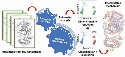
Machine learning has rapidly become a key method for the analysis and organization of large-scale data in all scientific disciplines. In life sciences, the use of machine learning techniques is a particularly appealing idea since the enormous capacity of computational infrastructures generates terabytes of data through millisecond simulations of atomistic and molecular-scale biomolecular systems. Due to this explosion of data, the automation, reproducibility, and objectivity provided by machine learning methods are highly desirable features in the analysis of complex systems. In this review, we focus on the use of machine learning in biomolecular simulations. We discuss the main categories of machine learning tasks, such as dimensionality reduction, clustering, regression, and classification used in the analysis of simulation data. We then introduce the most popular classes of techniques involved in these tasks for the purpose of enhanced sampling, coordinate discovery, and structure prediction. Whenever possible, we explain the scope and limitations of machine learning approaches, and we discuss examples of applications of these techniques.

Graphical Abstract

KEYWORDS:

• Biomolecular simulations
• molecular dynamics
• machine learning
• deep learning
• biophysics

1 Introduction

1.1. Why machine learning techniques are useful in analysis of biomolecular simulation data?

The first protein structure was discovered in 1958. In 2020, the number of resolved protein structures in the PDB database was already about 170,000 [1]. For a long time, these impressive structural data have highlighted our understanding of these biological molecular machines that control processes in living systems at the molecular level.

However, understanding the function of proteins requires that their dynamic activation process be elucidated. For this purpose, one of the best, if not the best method is molecular dynamics (MD) [2], which uses structural data as a starting point and puts the structures into motion. MD simulations are an outstanding method to study the dynamics not only of proteins but of all biologically relevant molecules. A good example of this broad field of application is the elucidation of the dynamic functions of cell membranes. Cell membranes comprised lipids act as a functional environment for many membrane-associated proteins, modulating the activation and function of proteins. At the same time, cell membranes are rich in glycans and interact with numerous signaling molecules as well as water, with essentially all biologically relevant molecular types contributing to the function of the membranes. Thus, it is not surprising that MD methods have been used exceptionally extensively to elucidate the structural and dynamic properties of cell membranes [3].

Pioneering applications of the MD technique explored simulation models over a time scale of picoseconds; however, modern computational infrastructure using, e.g. distributed computing [4] or specialized architectures [5,6] can generate simulation trajectories that extend up to the millisecond timescale [7,8]. At the same time, system sizes studied in MD simulations have become quite impressive, as is exemplified by simulations of molecular assemblies comprised of ~20 million particles [9]. Consequently, molecular simulations can generate terabytes of dynamic information: biomolecular Big Data. The explosion in the amount of information has created an exceptional challenge for investigators analyzing these data.

In life science, the goals of MD simulations are to identify the physiological processes of complex biomolecular assemblies and to unveil their functions [10]. A typical outcome of analyzing MD simulations is a robust statistical model that provides intuitive understanding into how the architecture of the biomolecular assembly gives rise to its function. Machine learning (ML) techniques [11] are one of the primary tools of computational scientists investigating large simulation data sets. ML techniques are algorithmic and automated, which is where the machine part of ML derives its origin. The learning part refers to detection of hidden patterns and structures in the data that the investigator wishes to unveil. ML techniques are data driven in that they rely on the presence of relevant statistical information contained in the data at hand.

Assuming that the available data is of high quality, there are three important reasons why ML techniques are useful. The first is reproducibility and objectivity. In the case of MD simulations, ML methods allow for a systematic selection of a model. This contrasts with visualizing simulation trajectories to try hunt down the physical model with the help of investigator’s intuition. The second key advantage of ML techniques is interpretability. ML techniques can highlight the importance of the chosen structural features of the biomolecules representing the structure–function relationships between these features and the function in a statistically coherent form. Third, ML techniques are predictive, leading to quantitative and empirically verifiable models for biological processes. It is therefore not surprising that ML techniques have found very important applications in, among other things, elucidating the properties of membrane proteins [12,13].

In Sections 2–4, we consider several important topics in more detail, but before doing so let us first discuss how machine learning can be linked to biomolecular simulations in a practically meaningful way.

1.2. Machine learning combined with biomolecular simulations

The idea of combining MD and ML is not novel [14–18]. Biomolecular simulation techniques, including MD methods, are a part of a broader discipline of statistical physics where statistical learning/ML tools have been used for decades to analyze data. But due to the rapidly increasing popularity of the ML paradigm, there has been a remarkable influx of well-established ML techniques from other scientific branches to analyze the data generated by biomolecular MD simulations.

ML techniques are regularly used for simplification of simulation data. This task is complicated due to the large dimensionality of the molecular structures that typically contain thousands to millions of particles. It is not unusual that the effective dimensionality of the biomolecular assembly is in the order of 10⁶. Furthermore, the thermal noise present in simulations of model systems can obscure the weak correlations that one would like to unveil. Even if a researcher has strong biological knowledge, it is very difficult to elucidate the mechanism of action of the problem under study from a mere visual examination. In fact, such a study may even lead to an interpretation based more on the researcher’s assumptions than on the actual research data. High-dimensional data sets are also susceptible to the curse of dimensionality [19], leading to difficult inference of a robust model for an underlying phenomenon.

ML addresses these issues through Dimensionality Reduction (DR) methods, which form an important pillar in the repertoire of ML techniques. DR methods ease visualization and analysis of high-dimensional data. In DR tasks, high-dimensional representations are mapped to a space of ‘useful properties’ (see below) through either a linear or a non-linear transformation. This new representation has a smaller effective dimension than the original one. Those with a background in statistical physics and/or the development of coarse-grained simulation models can see a connection to the concept of coarse graining. The properties associated with DR transformations are based on the choice of a metric that measures the encoding of the potentially useful information present in the original data set. The effective dimensionality is then determined by minimizing the number of chosen dimensions while maximizing the information of interest. A simple metric of this kind can be, e.g. the one that extracts variance or temporal autocorrelation of the simulated process, resulting in the identification of a lower-dimensional space that encodes simulation data with fewer degrees of freedom. In most cases on DR techniques, the investigator can highlight which structural components in the biomolecular system are most information rich and can discard the noise resulting from the leftover components. DR techniques are often used to identify collective modes, which represent highly correlated movements within or between biomolecules. Collective modes provide a means to easily visualize the interesting dynamics of a biomolecular system and an objective way to emphasize the importance to certain structural regions of the molecular system. In the above discussion, the concept of a biomolecular system can be either a single molecule or a structure formed by several molecules.

Another problem in processing biomolecular simulation data is understanding the effects of modifications of simulation conditions. How does a mutation of a residue or a change of pH affect the simulation data? Such a question is addressed by ML through Classification and Clustering tasks. When the membership of a data point to a certain category is known, classification tasks can be used to learn the relation between the assignment and the datapoint. For example, in the case of MD simulations of protein mutants, classification techniques can highlight the mutation-induced differences in the simulation data. Yet, the categories needed in the analysis are frequently unknown and need to be inferred from the simulation data. In the case of MD simulations, this problem boils down to identifying metastable states in the data using clustering tasks. Clustering can be carried out by clarifying the geometrical similarities in molecular structures or by employing some function computed from the structures. Clusters obtained from such an examination allow analysis of simulations based on the occupancy of the categories inferred from the data. Such clusters represent the metastable thermodynamic states sampled by the simulations. Like DR, clustering techniques are competent visualization and interpretation tools. Identifying the structural features that define these clusters provides insight into the underlying biological mechanism. Additionally, clustering can be used to identify the need for further sampling in the regions of the conformational space where current sampling is inadequate. Such an approach leads to a data-driven exploration of the conformational space and forms the basis of many enhanced sampling techniques.

An application of ML techniques relevant to MD simulation is regression. Regression can be defined as the construction of a parametric model inferred from the data that relates a set of predictor variables called regressors to a set of explained or predicted variables. Regression tasks are particularly useful when a function commensurate with some empirical observable is known and can be calculated from the structural data in the simulations. In such a scenario, the regression model can highlight the relative importance of structural features that take part in modulating the calculated function. Again, due to the high dimensionality of the structural space, inferring a robust regression model is a challenging task. Given this, regression models are augmented by first reducing the dimensionality of the space with DR techniques.

1.3. Machine learning with artificial neural networks

A special area of interest to the ML investigator are a class of techniques called Artificial Neural Networks (ANNs) [20], which are important to discuss separately. An artificial neural network (ANN) is designed to simulate the way our brain analyzes and processes information. It generates a map, which connects input data to a desired output through connections between artificial neuron nodes. The idea of an artificial neuron is inspired by biological neurons in the sense that an artificial neuron tries to model the activation process of genuine neurons with a simple computational model, where the downstream node in the ANN ‘activates’ or ‘deactivates’ the upstream node after receiving the input. This activation function simulates the activation potential at the synapse. In ANNs, the activation function can be linear or non-linear. Non-linear activation functions are used to apply a non-linear transformation to the input data, thus increasing the ability of the model to encode complex relationships between the input and the output.

In its basic form, ANNs are constructed in a simple three-layered form. The operation is based on an input layer, which connects to a hidden layer which transforms the data and is connected to an output layer, which is used to generate the actual prediction of the ANN. The hidden layer has several parameters that determine the transformations made to the input data. These parameters are trained in a supervised manner using a training set. Finally, the trained model is optimized and tested with validation and test data.

Over the past two decades, ANNs have become very powerful in forecasting tasks due to the introduction of several algorithmic improvements and increased hardware efficiency. The form in which ANNs are most often used is the so-called Deep Neural Networks (DNNs) [21] with multiple hidden layers. DNN activation functions are carefully selected nonlinear functions such that each hidden layer applies a sequential nonlinear transformation to the signal received from the previous layer. There are several architectural ways to achieve this, each of which creates a computational map that performs mathematical operations on the input in different ways. The most common of these architectures used for structural data are the Recurrent Neural Networks (RNNs), Convolutional Neural Networks (CNNs), and Autoencoders [21].

1.4. Practical aspects

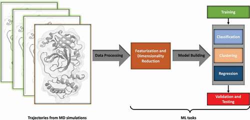
In terms of practical implementation, ML methods typically have a fixed workflow (Figure 1). The first step in every ML technique is featurization. In this step, the raw data with T samples is transformed into N features, which are the knowledge-rich components of the data. We expect the features to be involved in the underlying model which generates the observed data. The feature vector, which has dimensions of N x T, is divided into non-overlapping groups, labelled the training, testing and validation sets. The training set is subjected to ML analysis to infer a statistical model. Parameters not determined by the ML technique and introduced by the investigator (called hyperparameters) are tested and optimized on the validation set to determine the best performing set of hyperparameters. Finally, the accuracy of the model is tested in a series of tests that contain data that the model has never seen, to avoid overfitting.

Figure 1. Typical Machine Learning Workflow. Data generated from simulation trajectories is first represented by selecting certain features, usually reducing the dimensionality. Data is then chosen for training the ML tasks to generate a model, which is optimized for its hyperparameters, validated, and tested for overfitting.

ML techniques are exceptionally useful in solving a wide variety of problems related to analysis of complex MD simulation data, such as to discover reaction coordinates, to carry out coarse graining, and in reconstructing free energy surfaces that underlie the thermodynamics and kinetics of biomolecules.

Below, we focus on several ML tasks (Dimensionality Reduction, Clustering, Classification, and Regression) and their ability to address problems commonly encountered in MD simulations. We discuss popular techniques employed in these tasks and provide a brief overview of the studies that utilize ML. We conclude with a discussion of selected concrete applications, where machine learning has been used to analyze biomolecular simulation data.

2. Dimensionality reduction

Dimensionality reduction (DR) tasks transform data from a high-dimensional space onto a low-dimensional description. The general problem in DR is to generate a map of the form:

(1) $\begin{array}{c}{X}_N\to Y_d\end{array}$(1)

where N is the original dimensionality of the feature space, d is the reduced dimensionality of the new space, and X are the coordinates of the original and Y the coordinates of the new embedding. Such a transformation is conditioned on reconstructing a metric linked to information present in the original data. Although DR is required to reduce the effective dimensionality of the problem, the new space may have the same dimensionality as the original one. In this case, dimensionality reduction is accomplished by choosing an appropriate subspace that maximizes the reconstruction of the selected metric. DR techniques are some of the most common ML tools employed in the field of biomolecular simulations. They are often the first stage in the analysis of simulation data on which regression, classification, and clustering models are built. DR techniques can reveal the underlying structure of the conformational space, removing effects of information-poor dynamics of the biomolecule or biomolecular system, which is often interpreted as noise. The dimensions that remain after dimensionality reduction can also be used as a proxy for reaction coordinates or order parameters that define the paths connecting metastable states in the configurational space of biomolecules (or a biomolecular system). Here, we continue by discussing a common DR technique called principal component analysis.

2.1. Principal component analysis

Principal component analysis (PCA) [22] is one of the most popular techniques for reducing dimensionality in a wide variety of problems involving high-dimensional data. PCA has been used in a wide range of applications in the analysis of biomolecular simulation data. In their review, Stein et al. introduce numerous applications of PCA [23]. Since its inception in the field of data science, it has evolved from a standalone technique to an integral part of a larger workflow. Here we delve deeper into PCA compared to other methods since the terminology and ideas used in PCA are common to many techniques.

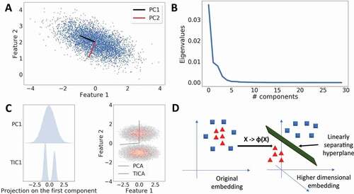
PCA is an ‘unsupervised’ statistical learning technique. The term unsupervised refers to the lack of requirement of a response variable to build a model. The central idea of PCA is the assumption that the variance of the data set is a proxy for the useful information contained within. PCA defines a linear and a dimensionality preserving transformation that generates a new coordinate system. Along the axes of this new coordinate system, the variance present in the original data set is maximized (Figure 2A). The input for PCA is the simulation trajectory data:

(2) $\begin{array}{c}{X}_{\mathrm{d}\mathrm{a}\mathrm{t}\mathrm{a}}\left(t\right)={\left(X_{i,\mathrm{d}\mathrm{a}\mathrm{t}\mathrm{a}}\left(t\right)\right)}_{i=1,\dots ,N}\end{array}$(2)

Figure 2. Dimensionality Reduction with Machine Learning. A. PCA is used to detect directions of highest variance. In a two-dimensional case, PCA resolves the variance into two orthogonal Principal Components (PCs). B. Typical eigenvalue spectrum obtained from PCA. PCA can be used to reduce dimensionality by selecting a cut-off, where the variance starts to go asymptotically to zero. C. Comparison of PCA and tICA methods on a two-well potential. Left: Projection of the first PC and tIC on the data. The first tiC correctly identifies the two minima in the free energy surface (FES). Right: tIC finds the direction along the two minima in the FES. D. Kernel PCA solves the PCA problem by first applying a non-linear transform on the data that embeds the data into a higher-dimensional space, where a hyperplane can linearly separate the data points which were not linearly separable earlier.

where X_data is the N-dimensional structural data at time t and X_i,_data are the components of the data. For biomolecular simulations, the components are the three spatial coordinates of all atoms in the structure. The recipe of PCA starts from centering the data:

(3) $X\left(t\right)=X_{\mathrm{d}\mathrm{a}\mathrm{t}\mathrm{a}}\left(t\right)-{⟨X_{\mathrm{d}\mathrm{a}\mathrm{t}\mathrm{a}}\left(t\right)⟩}_t$(3)

where $⟨.{⟩}_t$ is the expectation value computed over the entire data set. A covariance matrix ($C_{ij}^{\left(0\right)}$) is then built from the centered data:

(4) $C_{ij}^{\left(0\right)}={⟨X_i\left(t\right)X_j\left(t\right)⟩}_t$(4)

Using the covariance matrix, one obtains a diagonal matrix via eigen-decomposition. The diagonal matrix contains the eigenvectors ($r_i$) and the corresponding unordered eigenvalues (${\lambda }_i$), which are the variances along the eigenvectors. This decomposition is the solution to the eigenvalue problem:

(5) $\begin{array}{c}{C}^{\left(0\right)}{r}_i={\lambda }_i{r}_i\end{array}$(5)

This decomposition creates a linear transformation that rotates the coordinate system and aligns it along the direction that maximizes variance. The eigenvalues are the new variances along the transformed coordinates. A typical eigenvalue spectrum obtained from PCA is shown in Figure 2B. The eigenvectors are the new axes of this space and as such are orthogonal to each other. The new dimensions obtained in this manner are uncorrelated. A reduced dimensionality is now obtained by imposing restrictions on the eigenvalues. The eigenvalues are first ordered in a descending fashion. Then the variance explained by the largest k eigenvalues (out of n) can be used as a cut-off, such as the level of 95%, to determine the effective dimensionality:

(6) $\begin{array}{c}\sum _{i=1}^k{\lambda }_i/\sum _{i=1}^n{\lambda }_i\ge 0.95\end{array}$(6)

The eigenvectors are collective or correlated modes present in the data. Assuming that the subject of the study is a molecule, then these modes can be visualized by extrapolating the structure of the molecule along the eigenvectors.

As an exploratory technique, it is common to plot the projections of the data on the first two eigenvectors. This 2D-projection plot is then used as a basis for a quantitative classification, clustering, or regression task. As PCA eigenvectors represent the ‘largest’ motions in terms of variance, they are often used as reaction coordinates. These essential coordinates [24–27], as they are often called, are used for enhanced sampling of the simulation space [26,28]. There are two techniques where they have been used this way, namely conformational flooding [29] and a variant of metadynamics [30–32] that is based on the use of essential coordinates. In these methods, a biasing potential is applied to explore the coordinate represented by the eigenvector, which drives the simulation to explore the conformational space along the direction of the largest variance.

A problem that is inherent to many ML techniques is feature selection. In PCA this decision appears in the choice of coordinates to build the covariance matrix. For most biomolecules, this boils down to the use of non-hydrogen atoms. For proteins, as a rule of thumb, one often uses the cartesian coordinates of the backbone or the C-alpha atoms for this purpose. Alternatively, in techniques such as dPCA [33–36], the coordinates used are the dihedral angles of the protein.

PCA is a straightforward, compelling, and intuitive approach for DR and is used in combination with many ML techniques as a filter for simplifying the problem before performing more complex analysis. It is also a method of choice for exploration of the data and visualization of coordinated motions in the proteins. However, PCA has some significant pitfalls. Variance as a metric for the information contained in the simulations can lead the analysis astray. The largest variance modes in the sampled space might have no relation to the function of interest of the biomolecule. In fact, the subspace spanned by the effective dimensionality as calculated above might have little or no correlation with the function of interest. This has led investigators to choose alternative metrics for the information contained in the sample such as autocorrelations as described below. PCA is implemented in the scikit-learn [37] library of Python and distributed within the GROMACS [38] software package. The GROMACS package also provides convenient tools for visualization and analysis of the eigenvectors obtained from PCA.

2.2. Principal time-lagged independent component analysis

Time-lagged independent component analysis (tICA) [39] is somewhat similar to PCA. It selects the autocorrelation in the data as the metric for the information in the simulation data. tICA incorporates the time-structure from the simulations into the DR technique. tICA introduces a linear transformation on the data in a way analogous to PCA. The transformed space has the same dimensionality as the original space. For the calculation of tICA eigenvectors, a time-lagged autocorrelation matrix ($C_{ij}^{\left(\mathrm{\Delta }t\right)}$) is first computed from the centered data:

(7) $C_{\mathrm{i}j}^{\left(\mathrm{\Delta }t\right)}={⟨X_i\left(t\right)X_j\left(t+\mathrm{\Delta }t\right)⟩}_t$(7)

where $X_i\left(t\right)$ is the centered i^th coordinate at time t in the simulation trajectory. $X_j\left(t+\mathrm{\Delta }t\right)$ is the centered j^th coordinate at time t +$\mathrm{\Delta }t$ in the trajectory. The parameter $\mathrm{\Delta }t$ is the time-lag chosen when the autocorrelation matrix is constructed. The eigenvectors of this matrix, also called tICs, are a solution to the eigenvalue problem:

(8) $C^{\left(\mathrm{\Delta }t\right)}{r}_i=C^{\left(0\right)}{\lambda }_i{r}_i$(8)

where $C^{\left(0\right)}$ is the autocorrelation matrix computed without lag, ${\lambda }_i$ are the corresponding eigenvalues of the tICs, $r_i.$ To reduce dimensionality, an expression analogous to the above-discussed variance can be used to determine the effective dimension. Dimensionality of the subspace chosen for analysis is often determined by a hard cut-off, frequently set to 95% of the total autocorrelation in the system.

A major advantage of tICA is that its eigenvectors approximate the eigenfunctions of the underlying Markovian dynamics [40]. In other words, tICA aims to find the slowest-relaxing degrees of freedom in the time series data set. tICA eigenvectors hence represent the slowest dynamical modes as opposed to the PCA eigenvectors that maximize the variance present in the original data set as shown in Figure 2C. As tICA uses time correlation as the information metric, it is often utilized in DR tasks to build Markov State Models (MSMs) [41]. Further, they are often used in metadynamics-based methods to enhance sampling of the conformational space [42].

However, tICA suffers from a significant issue: the choice of the time-lag $\mathrm{\Delta }t$, which determines which kinetic processes are selected for constructing the new space. Any process slower than $\mathrm{\Delta }t$ is essentially ignored. Ideally, the time-lag $\mathrm{\Delta }t$ must be long enough so that the dynamics contained in tICA has the Markovian property of being memoryless, but also short enough so that the processes of specific interest are not neglected. There is currently no precise recipe to select $\mathrm{\Delta }t$ suitably. The construction models based on tICA, such as of MSMs, require considerable trial and error to choose the correct $\mathrm{\Delta }t$. A robust MSM constructed from tICA can be used to justify the choice of $\mathrm{\Delta }t$, although this is an expensive exercise. Nonetheless, tICA is a useful method for finding optimal components to reduce dimensionality as compared to PCA, as the time structure in the data can allow tICA to identify coordinates that can separate underlying metastable states in the data better than PCA. tICA is implemented for the purpose of analyzing biomolecular simulations in the PyEMMA package [43].

2.3. Kernel PCA and Kernel tICA

PCA and tICA are techniques that attempt to explain the metric of interest with a simple linear representation. However, correlations present in complex data sets are seldom linear. To capture non-linear correlations, a generalization of PCA based on the kernel trick [44] technique has been suggested. First, a non-linear function, called the feature function ($\phi$) is used to introduce additional dimensions to the data ($X$), where the function itself acts as an extra dimension:

(9) $\begin{array}{c}\phi :X\to f\end{array}$(9)

In this higher-dimensional space ($f$), the transformed points of the data are linearly separable by hyperplanes (Figure 2D). Yet this process requires expensive computations to calculate the map of the original data in the feature space and then to solve the PCA problem in that space. The kernel trick avoids this problem with selected choices of feature functions. It can be shown that calculating only the Gram matrix of the inner products of the feature functions is sufficient to calculate the eigenvectors of the embedding of the data in the feature space. These inner products are represented by kernel matrices ($k$):

(10) $k\left(x,x^{\prime }\right)={⟨\phi \left(x\right),\phi \left(x^{\prime }\right)⟩}_f$(10)

where $⟨.{⟩}_f$ is the expectation value calculated over the entire feature space. Examples of feature functions used for the kernel trick are polynomial kernels, Gaussian kernels, sigmoid kernels, and radial basis functions. Standard PCA is a special case of the polynomial feature function of the first order. In the same vein as kernel tICA, a kernel trick-based variant of tICA [45] has also been developed specifically to compute eigenfunctions of the Markovian dynamics in the simulation data without having to explicitly compute an MSM. Non-linear kernel-based methods provide a more robust estimate for the PCs, which explain the variance or autocorrelation better than their linear counterparts. However, the choice of the optimal feature function for a given data set is generally very difficult to guess a priori and is obtained by trial and error with available feature functions. It is also possible that for a given embedding of data, no feature function is suitable for a linear separation of the data.

Kernel PCA has been used in biomolecular simulations for identification of reaction coordinates of lactate dehydrogenase enzyme catalytic activity by Antoniou et al. [46]. Kernel PCA is implemented in the scikit-learn library of Python.

2.4. Manifold learning

Kernel PCA methods represent an attempt to capture the non-linearity of the space in which the data is embedded. However, the feature functions used for this purpose do it without any knowledge of the manifold in which this embedding exists. Methods that use the structure obtained from the data to gauge this manifold are more likely to capture patterns of the dynamics in a given data set. Some of the methods used successfully in biomolecular simulations for learning the manifold are Diffusion Maps [47] and Isomaps [48]. Diffusion maps calculate the connectivity between the datapoints by determining a diffusive model for transitions between data points using their time structure. The typical metric used to calculate the distances in the diffusion space is the root-mean square deviation (RMSD) between translationally and rotationally fitted structures. Diffusion maps have been used to calculate order parameters for alkanes [49], reaction coordinates in an alanine dipeptide toy model [50], and to characterize protein folding paths [51].

Isomaps, on the other hand, are constructed by finding a low-dimensional representation that preserves the shortest geodesic distances on the underlying manifold. This task is performed by building neighborhoods for a given point from the sampled data. A fixed number of neighbors are selected based on the smallest RMSD distance after rotationally and translationally fitting all structures. Isomap algorithms use the sampled configuration space to find shortest distances between any two points along a path connecting neighbors, and this distance is defined as the geodesic distance for any two structure pairs. Isomaps have been used to discover protein folding reaction coordinates [52], to apply enhanced sampling to popular frameworks such as metadynamics [53], and to infer collective coordinates from simulations [54] to supplement other analysis tasks. Implementations for many manifold learning tasks can be found in the scikit-learn package of Python.

2.5. Dimensionality reduction with autoencoders

An autoencoder [55] is a neural network that learns to copy its input to its output in a manner where the autoencoder reconstructs the input approximately, preserving only the most relevant aspects of the input data in the output copy. To this end, autoencoders typically use the ANN framework that uses data reconstruction as a metric instead of a function of the data, such as variance or autocorrelation. Unlike most other ANN techniques, autoencoders are unsupervised as the response (output) variable is identical to the input variable.

The parameters in the autoencoder (implemented as an ANN) are optimized by a loss function ($L$). In the simplest form of an autoencoder, it is the reconstruction error:

(11) $\begin{array}{c}L\left(x,x{ }^{\mathrm{\prime }}\right)=|x-x{ }^{\mathrm{\prime }}{|}^{2\hspace{0.17em}}\end{array}$(11)

where $x$ is the original data vector and $x{ }^{\mathrm{\prime }}$ is the predicted data vector. The loss function is very relevant in this context since the key principle of autoencoders is that they funnel the information present in the input through a lower-dimensional layer, called an encoding layer of an ANN. Minimization of the reconstruction error after such a passage enforces dimensionality reduction due to the smaller dimension of the encoding layer. The part of the ANN prior to the encoding layer is called the Encoder, while the part after it is called the Decoder. The effective dimensionality of autoencoders is determined by the size of the encoding layer. The encoding layer dimension is a hyperparameter, which is optimized as a part of the training of the ANN. Autoencoders such as most ANN applications are built with non-linear activation functions that can compress information present in the original data much more efficiently compared to linear methods such as PCA or tICA. In fact, autoencoders without non-linearities are directly analogous to PCA. Time-lagged autoencoders have been specifically constructed to mimic the properties of tICA [56].

Autoencoders are probably the most significant use of ANN techniques in the analysis of biomolecular simulations. They have been used by Chen et al. [57]. for coordinate discovery, where autoencoders perform enhanced sampling to calculate the free energy surface from newly discovered collective variables. The reweighted autoencoded variational Bayes for enhanced sampling (RAVE) [58] framework, based on variation autoencoders (VAEs) by Ribeiro et al., has been used to obtain physically interpretable reaction coordinates from simulations [59]. Autoencoders have been used in DR for further analysis such as clustering and constructions of Markov State models [60]. They have also been used to construct coarse-grained force fields to reproduce the energetics obtained from atomistic simulations [61]. Overall, autoencoders can be used as a model to predict and sample hitherto unobserved structures in the configurational space of biomolecules (Figure 3) [62]. Autoencoders are implemented in the scikit-neuralnetwork library in scikit-learn.

Figure 3. ANNs for Dimensionality Reduction. Autoencoder networks (shown in gray) are used for training a lower-dimensional representation of the simulation data by reconstructing sampled structures (deep blue) with decoded structures (light blue). A trained autoencoder can be used to generate a latent space representation of the data set (blue points), which can used to generate unseen latent space data (red points) to mine unsampled structures (red structures). Figure adapted from Degiacomi et al. [62].

3. Regression techniques

In studies of research questions dealing with biomolecular structure, one typically has some information about molecular properties that describe the function of the biomolecule. Alternatively, a feature extracted from the structure or dynamics of the system of interest can be used as a measure of its biological function. For example, for catalytic proteins a metric of enzyme activity can be the orientation of active residues. In the case of membrane channels, the channel conductance can be used as a direct measure of the permeability of the protein. In cases like these, regression techniques can be used to construct a mechanistic model of structure–function relationships. However, since these processes take place in a high-dimensional system, the noise caused by those degrees of freedom that do not contribute to biomolecular activity interferes with the construction of a robust multivariate regression model. Two ML techniques, both based on Functional Mode Analysis (FMA), are able to resolve this issue by reducing dimensionality.

3.1. PCA-based functional mode analysis

PCA-based FMA is a technique based on Principal Component Regression (PCR), a methodology that uses ordinary least squares (OLS) with the PCA components as regressors and a function calculated from the simulation data. PCR uses only a subset of the Principal Components (PCs) for the regression model and thus leads to reduction in the total variance present in the data by an amount equal to the variance present in the omitted components. This omitted variance is identified as noise resulting from those degrees of freedom in the data that have little or no correlation with the function of interest.

The recipe for PCR is simple. First, one calculates the PCs by performing PCA on the data. The PCs are then used as regressors in OLS regression against the function vector calculated for each data sample used for PCA. If all the PCs are used for the regression, then the PCR is identical to a multilinear regression model. If, however, only selected PCs are used, then variance reduction can be achieved. The selection of PCs is generally based on their eigenvalues. As a rule of thumb, the PCs with largest eigenvalues that result in a cut-off (e.g. 95%) of variance, as discussed above, are used as regressors. To gain a more robust model for the correlation between the function of interest and regressors, PCs can be added to the regression problem to create a more complex model until a target value of regression coefficient is achieved.

PCA-based FMA was implemented by Hub et al. [63], where they addressed the regression problem by calculating the Pearson regression coefficient and mutual information between the PC regressors and the target function. To interpret the model, PCA-based FMA generates an ensemble-weighted Maximally Correlated Mode (ewMCM), which represents the most probable collective motion correlated with the function of interest. This ewMCM is the direct stand-in for thermodynamically attested mechanical action of the biomolecule as depicted in Figure 4, where the PCR method was used to better understand the collective dynamics of the leucine-binding protein.

Figure 4. Principal Component Regression (PCR). A. PCR-based ensemble-weighted mode for the Leucine Binding Protein. B. Coefficient α_i of the contribution to the PCR model from the largest PCA eigenvectors. C. Eigenvalues of the PCs used to construct the PCR model. D. Contribution of the variance of the PCs to the variance of the collective mode. Figure adapted from Hub et al. [63].

3.2. PLS-based FMA

An obvious caveat of PCR-based methods is that the subspace used for regression is built independently of the function of interest. While PCs have for long been considered important for the function of biomolecules in the MD simulation community, high-variance PCs calculated from limited data may have little or no correlation with the responses used to train the PCR model. A model built solely from high-variance PCs will ignore low-variant PCs with high correlation to the function. This problem has been addressed in the statistical learning community with the help of the Partial Least Squares (PLS) methodology. PLS is a cross-decomposition method, i.e. unlike PCR where the regressors are identified by decomposing the data matrix first via PCA, PLS methods add the information from the response variables to the decomposition as well. This is done in an iterative process, where first a component of the data vector with maximum correlation with the response variables is identified. Then that component is subtracted from the data matrix and stored as a regressor. The process is then iteratively repeated for the reduced data matrix to find the next orthogonal component with maximum correlation with the response variable. The final model in the PLS method is a linear combination of all the components extracted through this algorithm. The number of PLS components are dependent upon the required amount of correlation that needs to be explained from the data. Once this limit is reached, the investigator can stop the iteration process and choose the model with the current number of components.

PLS-based methods have an obvious advantage over PCR-based techniques. Components of the PLS model are of natural interest from the point of view of the mechanical model that investigators want to extract from the data. PLS-based methods provide a simple, yet elegant linear and interpretable relationship between the data and the response.

Krivobokova et al. [64] implemented this method for analyzing biomolecular simulations by incorporating it in the FMA framework introduced by Hub et al. In a certain sense, the method is an update to the PCA-based FMA. It has been shown that PLS-based FMA creates models of lower complexity to reach the correlation values discussed above. In the same manner as PCA-based FMA, an ewMCM can be computed from PLS-based FMA. This ewMCM can be visualized like PCA-based eigenvectors and provide mechanical insight into structure–function relationships in biomolecules. PLS-based FMA techniques have been used to understand how membrane channel proteins like aquaporins are regulated by pH [65] and mutations [66]. The PLS package is available in the scikit-learn library of Python, and also in the GROMACS software suite.

3.3. Force matching with ANNs as a regression problem

As an example of ANNs performing regression tasks where response variables are used to fit thermodynamic properties of biomolecules, one can consider force matching [67]. It is a technique where the parameters of a coarse-grained (molecular) force field are determined by matching the forces used in a coarse-grained representation with the forces obtained from a fine-grained (atomistic) representation. This process has been used, for instance, to reproduce forces calculated from expensive quantum-mechanical calculations in classical atomistic simulation models [68]. Recently, the force matching technique was used to reproduce atomistic forces in a coarse-grained representation using ANNs [69,70].

Wang et al. [71] developed a framework named CGnets that learns the free energy functional with the help of the force matching scheme (see Figure 5). In this framework, invariances derived from physics are introduced, namely a conservative potential of mean force and rotational and translational invariance. The former is accomplished by using a gradient-domain machine learning (GDML) approach, which enforces the forces computed at the atomistic level to match the forces generated by the coarse-grained representation. The latter is implemented by mapping the cartesian embedding of molecular coordinates on internal coordinates such as pairwise distances and dihedral angles that are rotationally invariant. The CGnets model is developed in a state corresponding to an implicit solvent. The free energy contribution of solvation is absorbed into the overall parametrization of the protein force field. Though this model has low transferability, it is a proof of principle experiment demonstrating the utility of ANNs as a regression model for parametrization of coarse-grained biomolecular simulation models. For the sake of completeness, it is worth mentioning the use of neural networks to coarse-grain the structure of biomolecules. Murtola et al. showed how self-organizing maps can be used to analyze atomistic representations of biomolecules to determine their simpler (coarse-grained) representations that include all the structural features that are most relevant to the function of the molecule [72].

Figure 5. ANNs for Regression. ANNs can be trained to develop coarse-grained force fields by the force matching method. Physical restrictions of translational and rotational invariance, and conservative forces, are imposed on the regression task performed by the CGnets architecture by a choice of internal coordinates and the GDML layer, whereby the atomistic force field is reduced to a coarse-grained force field. Figure adapted from Wang et al. [71]. Further permissions related to the material excerpted (https://pubs.acs.org/doi/full/10.1021/acscentsci.8b00913) should be directed to the ACS.

4. Classification and clustering techniques

A typical problem in analysis of biomolecular data is assignment of categories. Sometimes it is known a priori what category a particular data set belongs to. In these cases, the goal is to understand differences between distinct classes that all share a common featurization. It could be that the investigator is trying to develop a model where classification needs to be learnt so that an unclassified data set can be classified with the mode. Classification tasks guided by ML can accomplish both goals. In other cases, the challenge could be to identify some internal order and grouping within the data set. If so, can it be identified in an automated manner without any supervision? This is the question answered by clustering tasks. Yet, in most cases it is important to first simplify the tasks of clustering and classification by reducing the dimensionality of the data sets. Below we consider four popular instances of these techniques.

4.1. Partial least squares-based discriminant analysis

Partial Least Squares-based Discriminant Analysis (PLS-DA) [73] is an application of the PLS-based methods for the purpose of classification. PLS-DA is a supervised method that solves the same regression problem as PLS-FMA, when the response vector is discrete and categorical instead of being continuous. In the scenario where the class labels are qualitative, i.e. not mappable on real numbers, the investigator can assign one-hot vector representations to the classes for the purpose of finding a subspace that optimally separates the classes. In the same vein as PLS-based FMA, the complexity of the model obtained by PLS-DA can be increased by adding components until a target classification accuracy is reached. As an example of its applicability, one can consider a case of several simulations of mutations in proteins. A typical goal in this case could be to identify the subspace of the structural dynamics that optimally defines each mutant. In PLS-DA methodology each mutational simulation can be expressed as one-hot encoding. The PLS-DA algorithm provides a linearly separating hyperplane which can be used to identify the differences between simulations under varying but known conditions. PLS-DA has been used for separating the simulations of ubiquitin with bound and unbound partners as illustrated in Figure 6A [74], indicating its usefulness for classification tasks. More recently PLS-DA was used to determine dynamical differences in ligand-bound and unbound simulations of the PDZ2 domain and to identify differences in lysozyme mutants [75]. PLS-DA is implemented in the scikit-learn package of Python.

Figure 6. Classification and Clustering (Machine Learning) Techniques. A. Partial least squares-based Discriminant Analysis technique (PLS-DA) is used for identifying the collective mode that differentiates between bound and unbound ubiquitin simulations. Projection of the simulation data from the bound and unbound simulations on the difference vector given by the PLS-DA mode separates their distributions. Inset: The structural ensembles of ubiquitin binding region in the unbound and bound mode identified by the PLS-DA eigenvector. Figure adapted from Peters et al. [74]. B. Active and inactive states of the Src kinase are identified from MD simulations with clustering and then classified using a Random Forest (RF) classifier. Using a Gini index, importance is assigned to the residues that contribute most significantly to the classification. Figure adapted from Sultan et al. [76]. Further permissions related to the material excerpted (https://pubs.acs.org/doi/10.1021/ct500353m) should be directed to the ACS. C. L11 · 23S protein-complex is first subjected to dimensionality reduction. The simulation data are projected on the first two eigenvectors and then clustered with the k-means algorithm to identify the structure in the data. Figure adapted from Wolf et al. [35]. D. Gaussian Mixture Model-based clustering is used to identify the free energy minima in Calmodulin simulations using the InfleCS methodology. The GMM is built on a 2D surface using the coordinates reciprocal interatomic distances (DRID) and the linker backbone dihedral angle correlation (BDAC). The most likely transition pathways in these states are identified and plotted on the free energy surface. Figure adapted from Westerlund et al. [96]. Further permissions related to the material excerpted (https://pubs.acs.org/doi/abs/10.1021/acs.jctc.9b00454) should be directed to the ACS.

4.2. Decision trees

Decision trees [77] are a tree-like graph model, i.e. they have a network structure where each pair of nodes are connected only by one edge. Decision trees are used to perform both regression and classification tasks. When the target value of a parent node (also called the input node) is discrete, the decision tree performs classification. The child or the target nodes represent the known class labels. Decision trees are non-parametric models that advance the classification process by splitting the parent nodes into child nodes. The splitting is an algorithmic step that determines which class label will be assigned to a subset of the parent node. Splitting methods are chosen based on maximizing variance between the child node or maximizing gain in information due to the splitting.

Another popular metric for classification in decision trees is the Gini impurity index, which minimizes the probability of misclassification of an entry into a child node. If the splitting leads to optimal separation of the samples in the child nodes, any of these criteria can objectively report the fact. Decision trees are intuitive and simple to implement and interpret. However, they suffer from some severe problems. Decision trees are prone to overfitting when attempting to maximize the ability to classify data. This behavior results from creation of child nodes that contain only one or a few samples that can trivially satisfy the optimization criteria. It is possible to avoid overfitting by demanding that a given child node must contain at least a required minimum number of samples, and by regulating the maximum depth of branches that the trees can have. Also, decision trees generate piecewise constant approximations for the decision boundaries. As these boundaries are not continuous, decision trees are not able to extrapolate data very well.

Another prevalent issue with decision trees is the sensitivity to fluctuation in the training data. If the classification task requires complex decision boundaries, then the outcome of the decision tree becomes highly dependent on the structure of the training data and small changes in training can lead to different structures for the final model. This problem is solved by the so-called ensemble learning methods. Ensemble learning involves generation of multiple models from subsets of training data and identifying a consensus model from their ensemble. This approach is identical in spirit to bootstrapping methods and is thus also called Bootstrapping aggregation. Creating such tree ensembles leads to the Random Forest method [78]. The random forest technique has been used for analysis of biomolecular structural data to predict protein-protein interaction sites [79], to estimate protein-ligand binding energies [80], to predict phase diagrams of lipid mixtures [81] and to identify and classify binding modes of enzymes [82]. Decision tree classifiers based on random tress were also used to automate the selection of features of analysis as demonstrated for the Src kinase in Figure 6B, where this technique was used to pinpoint the residues characterizing its bound and unbound ensembles [76].

4.3. K-means/K-medoids

K-means [83] is a clustering technique that partitions the data $x$ into $k$ non-overlapping sets $C_i$. The boundary of each set is determined by its distance from a mean ${\mu }_i$ that is identified as a part of the K-means optimization algorithm, which attempts to minimize the variance of a subset of data. This condition is expressed as:

(12) $\begin{array}{c}\underset{C}{argmin}\sum _{i=1}^k\sum _{x\in C_i}|x-{\mu }_i{|}^2\end{array}$(12)

This term is called the Within Cluster Sum of Squares (WCSS). The number of cluster means is a hyperparameter that must be chosen in the beginning of the algorithm. K-means begins with an initialization by first assigning cluster means randomly and assigning nearest points to that mean, creating a subset or a cluster. The assignment requires that for a given set of means, the WCSS score is minimized for that assignment. This is followed by an iterative step, where the cluster means are updated to be the geometric means of the current subsets:

(13) $\begin{array}{c}{\mu }_{\mathrm{i}}^{\left(n+1\right)}=\frac{1}{\left|C_i^{\left(n\right)}\right|}\sum _{x_j\in C_i^{\left(n\right)}}{x}_j\end{array}$(13)

where n is the current step. Once this update step has converged to a stable set of means, the clusters are assigned to the final values of the means calculated in the last step. K-means is most frequently used for the selection and assignment of microstates in Markov State Models [84] as well as for structural clustering tasks [85–88]. An example of state assignment is depicted in Figure 6C, where the conformational space first reduced with PCA is clustered with K-means [85].

K-medoids is a related technique, where the means are not assigned to arbitrary points but instead assigned to real data points in the space, i.e. to real structures in the simulations. Otherwise, K-medoids follows the same algorithmic steps as K-means. An advantage of K-medoids is that the investigator can directly select the structures associated by the medoids as a representation of the cluster. K-means-like algorithms can suffer from a few difficulties, which need to be addressed with manual inspection of the output of the algorithm. Most importantly, K-means can get trapped in local minima and lead to sub-optimal results. This problem can be resolved by running the algorithm several times with different choices of the initialization and then minimizing the final WCSS obtained.

4.4. Density based clustering

Density-based (DB) clustering methods are an alternative to the previously presented neighborhood-based algorithms. The goal of DB-clustering algorithms is to identify high-density areas separated by regions of low density in the given space. The advantage of this approach is that it allows the algorithm to identify clusters of arbitrary shape, as opposed to neighborhood-based searches, which work best when the data samples can be characterized by a more or less convex shape. The most popular technique among DB clustering appears to be the Density Based Scan Algorithm with Noise (DBSCAN) [89]. In this algorithm, the idea is to first identify ‘core samples’ in the data, which corresponds to regions of space with a fixed number of points within a chosen radius ε. Once identified, in the second step one merges the core samples that share bordering points in the ε-neighborhood generating the cluster. The process is fully deterministic. The DBSCAN method is more resistant to noise components resulting from transition regions between the identified core clusters as compared to methods based on neighborhood searches. However, it can lead astray under conditions of sparse sampling that tend to characterize data that have a high variance in density. Also, DBSCAN does not scale well with increasing dimensionality of the space due to the complexity of corresponding neighborhood searches. DBSCAN has been used to identify specific ligand binding sites [90] for proteins and DNA [91]. It has also been used to study clustering of the conformations of small peptides in simulations [92].

An improvement of the DBSCAN algorithm is the HDBSCAN [93] technique – Hierarchical Density Based Scan Algorithm with Noise. In this technique, the epsilon radius restriction is removed allowing for a more robust search of the space for clusters. HDBSCAN has been used as an effective tool to visualize complex dynamics in MD simulations [94].

4.5. Gaussian mixture models

Gaussian Mixture models (GMMs) [83] are mixture models in the sense that they create linear combinations of Gaussian probability distributions for unsupervised ML tasks such as clustering. A typical GMM model has the form:

(14) $p\left(x\right)=\sum _{i=1}^K{\varphi }_i\mathcal{N}\left(x|{\mu }_i,{\sigma }_i\right)$(14)

where ${\varphi }_i$ is the weight of the i^th component in the model, $\mathcal{N}$ is a Gaussian density characterized by mean ${\mu }_i$ and standard deviation ${\sigma }_i$, and x is a datapoint whose probability, $p\left(x\right)$, is evaluated with this model. When applied as a solution to a clustering problem, a GMM identifies a latent or a hidden variable associated with the data set which corresponds to the cluster label, i = 1 … K of the datapoints. This allows the problem to be set up with a Bayesian framework, where the goal is to calculate the parameters ${\mu }_i\mathrm{a}\mathrm{n}\mathrm{d}{\sigma }_i$ for each cluster given the observed data. The solution can be obtained by solving a Maximum Likelihood estimator (MLE) for the parameter vectors. Generally, this is accomplished by using the Expectation Maximization (EM) algorithm.

Due to their intuitive structure and algorithmic simplicity, GMMs are an often-used solution to analyze data from biomolecular simulations. GMMs have been used for developing reaction coordinate discovery algorithms, such as Gaussian Mixture-based Umbrella Sampling [95], InfleCS [96] (Figure 4D) and GAMBES [97], where the GMM is used for clustering a reduced coordinate space to discover metastable states. GMMs have been coupled with ANNs to get interpretable embeddings from Autoencoder-based models as well [60]. GMM implementations are available in the scikit-learn library of Python.

4.6. ANN-based classification

ANNs can be trained to provide a powerful means to classify labelled data. A straightforward application of this idea is classification of biomolecular simulations under varying but known conditions. Plante et al. [98] used an architecture based on Convolutional Neural Networks (CNNs) (Figure 7) to identify residues of G-protein coupled receptors (GPCRs) based on changes introduced by ligand binding. First, GPCRs are scrambled rotationally and translationally to remove the bias from their coordinates. Then a transformation from the cartesian X, Y, Z coordinates to an RGB color code is applied for each atom of the GPCR to create a pixel in a 2D representation. This new representation is well suited for a CNN-based classification analysis, which generates a nonlinear map from the 2D picture to the known class assignment of the GPCR. Once trained with the simulation data set, the CNN learns a non-linear function for classification.

Figure 7. ANNs for Classification. ANNs used for classification of GPCRs based on differences in a bound agonist. The geometric coordinates are first encoded into the RGB code to generate a two-dimensional image. Using a convolutional neural network architecture, the map between the image and the corresponding level is learnt. Sensitivity analysis is used to retrace the pixels in the image and then from them the corresponding residues that are mainly responsible for the classification task. Figure adapted from Plante et al. [98].

Using a technique called Saliency maps [99], Plante et al. were able to backtrack to the relative importance of the input pixels on the classification outcome, which can then be translated to the identity of specific atoms of GPCRs. Such an application reveals the increasing interpretability that is being introduced in ANN-based modelling of structural data.

5. Conclusions

ML techniques can be integrated into all problem categories dealing with biomolecular simulations. ML techniques are used to identify key structural features for analysis, and they have a significant advantage in improving the signal-to-noise ratio by eliminating excessive degrees of freedom from the explored system or process. ML tools are particularly useful when investigators need to differentiate between simulation data sets without their own prejudices affecting the outcome of the analysis. When the goal of analysis is to associate the simulation data to continuous labels, highly interpretable regression techniques can be used to learn the structure–function relationships.

With the innovative architectures adopted by Artificial Neural Networks, ML can contribute to more than just the analysis of simulation data. For instance, ANNs can be built to coarse-grain structural representations of biomolecular systems by imposing physical constraints that ensure physically correct simplified models. This approach has a lot of potential, but so far it has not been used much. The main weaknesses of the ANN approach are the need of high-quality–high-volume data and interpretability. The first of these two problems can be avoided quite easily, because the amounts of data produced by biomolecular simulations are constantly increasing. As far as interpretation is concerned, enormous progress has been made, for example, thanks to sensitivity analysis, which allows researchers to trace the function learned by the ANN to the initial input given to it.

What does all this mean for biomolecular simulations? This question is naturally illuminated by where data science is currently advancing. The goal of data science is to have an automated, reproducible, and objective approach to both hypothesis generation and testing. These goals are ubiquitous in all branches of natural sciences, and data science most clearly intersects with those branches where data productivity (high throughput data generation) is high. The advantage of ML methods is that they establish a concrete pipeline for analysis, the structure of which is both modular and sufficiently flexible to rapidly test new approaches. More importantly the ‘pipes’ in this pipeline are generic and accept both qualitative and quantitative data. These considerations mean that experimenting with multiple approaches simultaneously has become relatively convenient. What makes the ML pipeline robust is the use of a well-defined testing and validation framework, which ensures that the models developed are efficient and suitable for the chosen task. In addition, in the times of Open-Source software development, all of these tools, protocols, and algorithms are readily available in public repositories, in a convenient format, and flexibly implemented. Models built from biomolecular simulation data are statistical, and the ML approach is ideally suited for formalizing their formulation. In our view, as a result of all this, ML methods have the potential to control the future of the biomolecular simulation field.

Acknowledgments

We thank CSC - IT Center for Science (Espoo, Finland) for computing resources. We thank the Sigrid Juselius Foundation, the Academy of Finland (project no. 331349), Human Frontier Science Program (project no. RGP0059/2019), and the Helsinki Institute of Life Science (HiLIFE) Fellow program for financial support (I.V.). We also thank the University of Helsinki (3-year project grants) and the EU (Marie Skłodowska-Curie Fellowship program) for funding (SK).

Disclosure statement

No potential conflict of interest was reported by the author(s).

Correction Statement

This article has been republished with minor changes. These changes do not impact the academic content of the article.

Additional information

Funding

This work was supported by the Academy of Finland [331349]; Human Frontier Science Program [RGP0059/2019]; University of Helsinki [3-Year Grants]; European Union (Marie Skłodowska-Curie Actions (MSCA)) [101033606].

References

- PDB Statistics: Overall growth of released structures per year. Nov 30, 2020. https://www.rcsb.org/stats/growth/growth-released-structures.
- Hollingsworth SA, Dror RO. Molecular dynamics simulation for all. Neuron. 2018;99:1129–31.
- Enkavi G, Javanainen M, Kulig W, et al. Multiscale simulations of biological membranes: the challenge to understand biological phenomena in a living substance. Chem Rev. 2019;119:5607–5774.
- Shirts M, Pande VS. Screen savers of the world unite. Science. 2000;290:1903–1904.
- Shaw DE, Deneroff MM, Dror RO, et al. Anton, a special-purpose machine for molecular dynamics simulation. Commun ACM. 2008;51:91–97.
- Shaw DE, Grossman JP, Bank JA, et al. Anton 2: raising the bar for performance and programmability in a special-purpose molecular dynamics supercomputer. SC’14: Proceedings of the International Conference for High Performance Computing, Networking, Storage and Analysis, pp. 41–53 (2014). New Orleans, USA. doi: 10.1109/SC.2014.9.
- Shaw DE. Millisecond-long molecular dynamics simulations of proteins on a special-purpose machine. Biophys J. 2013;104:45a.
- Lane TJ, Shukla D, Beauchamp KA, et al. To milliseconds and beyond: challenges in the simulation of protein folding. Curr Opin Struct Biol. 2013;23:58–65.
- Chandler DE, Strümpfer J, Sener M, et al. Light harvesting by lamellar chromatophores in Rhodospirillum photometricum. Biophys J. 2014;106:2503–2510.
- Dror RO, Dirks RM, Grossman JP, et al. Biomolecular simulation: a computational microscope for molecular biology. Ann Rev Biophys. 2012;41:429–452.
- Hastie T, Tibshirani R, Friedman J. The elements of statistical learning: data mining, inference, and prediction, Second Edition. Springer Series in Statistics; New York, NY. 2009. DOI:10.1007/978-0-387-84858-7.
- Jumper J, Evans R, Pritzel A, et al. Highly accurate protein structure prediction with AlphaFold. Nature. 2021;596:583–589.
- Hegedűs T, Geisler M, Lukács G, et al. AlphaFold2 transmembrane protein structure prediction shines. bioRxiv. 2021 2021.08.21;457196. DOI:10.1101/2021.08.21.457196.
- Haiech J, Koscielniak T, Grassy G. Use of TSAR as a new tool to analyze the molecular dynamics trajectories of proteins. J Mol Graph. 1995;13:46–48.
- Gordon HL, Somorjai RL. Fuzzy cluster analysis of molecular dynamics trajectories. Proteins. 1992;14:249–264.
- Troyer JM, Cohen FE. Protein conformational landscapes: energy minimization and clustering of a long molecular dynamics trajectory. Proteins. 1995;23:97–110.
- Karpen ME, Tobias DJ, Brooks III,CL. Statistical clustering techniques for the analysis of long molecular dynamics trajectories: analysis of 2.2-ns trajectories of YPGDV. Biochemistry. 1993;32:412–420.
- Torda AE, van Gunsteren WF. A lgorithms for clustering molecular dynamics configurations. J Comput Chem. 1994;15:1331–1340.
- Bellman R. Dynamic programming. Science. 1966;153:34–37.
- McCulloch WS, Pitts W. A logical calculus of the ideas immanent in nervous activity. Bull Math Biophys. 1943;5:115–133.
- Lecun Y, Bengio Y, Hinton G. Deep learning. Nature. 2015;521:436–444.
- Jolliffe IT, Cadima J. Principal component analysis: a review and recent developments. Philos Trans R Soc A Math Phys Eng Sci. 2016;374:20150202.
- Stein SAM, Loccisano AE, Firestine SM, et al. Principal components analysis: a review of its application on molecular dynamics data. Annu Rep Comput Chem. 2006;2:233–261.
- Lange OF, Grubmüller H. Can principal components yield a dimension reduced description of protein dynamics on long time scales? J Phys Chem B. 2006;110:22842–22852.
- Sittel F, Jain A, Stock G. Principal component analysis of molecular dynamics: on the use of cartesian vs. internal coordinates. J Chem Phys. 2014;141:014111.
- Amadei A, Linssen ABM, de Groot BL, et al. An efficient method for sampling the essential subspace of proteins. J Biomol Struct Dyn. 1996;13:615–625.
- Amadei A, Linssen ABM, Berendsen HJC. Essential dynamics of proteins. Proteins. 1993;17:412–425.
- Daidone I, Amadei A. Essential dynamics: foundation and applications. Wiley Interdiscip Rev Comput Mol Sci. 2012;2:762–770.
- Lange OF, Schäfer LV, Grubmüller H. Flooding in GROMACS: accelerated barrier crossings in molecular dynamics. J Comput Chem. 2006;27:1693–1702.
- Branduardi D, Bussi G, Parrinello M. Metadynamics with adaptive Gaussians. J Chem Theory Comput. 2012;8:2247–2254.
- Spiwok V, Lipovová P, Králová B. Metadynamics in essential coordinates: free energy simulation of conformational changes. J Phys Chem B. 2007;111:3073–3076.
- Yang YI, Shao Q, Zhang J, et al. Enhanced sampling in molecular dynamics. J Chem Phys. 2019;151:070902.
- Altis A, Nguyen PH, Hegger R, et al. Dihedral angle principal component analysis of molecular dynamics simulations. J Chem Phys. 2007;126:244111.
- Sittel F, Filk T, Stock G. Principal component analysis on a torus: theory and application to protein dynamics. J Chem Phys. 2017;147:244101.
- Wolf A, Kirschner KN. Principal component and clustering analysis on molecular dynamics data of the ribosomal L11·23S subdomain. J Mol Model. 2013;19:539–549.
- Mu Y, Nguyen PH, Stock G. Energy landscape of a small peptide revealed by dihedral angle principal component analysis. Proteins. 2005;58:45–52.
- Pedregosa F, Varoquaux G, Gramfort A, et al. Scikit-learn: machine learning in Python. J Mach Learn Res. 2011;12:2825–2830.
- Abraham MJ, Murtola T, Schulz R, et al. Gromacs: high performance molecular simulations through multi-level parallelism from laptops to supercomputers. SoftwareX. 2015;1–2:19–25.
- Molgedey L, Schuster HG. Separation of a mixture of independent signals using time delayed correlations. Phys Rev Lett. 1994;72:3634–3637.
- Pérez-Hernández G, Noé F. Hierarchical time-lagged independent component analysis: computing slow modes and reaction coordinates for large molecular systems. J Chem Theory Comput. 2016;12:6118–6129.
- Noé F, Clementi C. Kinetic distance and kinetic maps from molecular dynamics simulation. J Chem Theory Comput. 2015;11:5002–5011.
- Sultan MM, Pande VS. TICA-metadynamics: accelerating metadynamics by using kinetically selected collective variables. J Chem Theory Comput. 2017;13:2440–2447.
- Scherer MK, Trendelkamp-Schroer B, Paul F, et al. PyEMMA 2: a software package for estimation, validation, and analysis of Markov models. J. Chem. Theory Comput. 2015;11:5525–5542.
- Hofmann T, Schölkopf B, Smola AJ. Kernel methods in machine learning. 1. Ann Stat. 2008;36:1171–1220.
- Schwantes CR, Pande VS. Modeling molecular kinetics with tICA and the kernel trick. J Chem Theory Comput. 2015;11:600–608.
- Antoniou D, Schwartz SD. Toward identification of the reaction coordinate directly from the transition state ensemble using the kernel PCA method. J Phys Chem B. 2011;115:2465–2469.
- Coifman RR, Lafon S, Lee AB, et al. Geometric diffusions as a tool for harmonic analysis and structure definition of data: diffusion maps. Proc. Natl. Acad. Sci. 2005;102:7426–7431.
- Tenenbaum JB, De Silva V, Langford JC. A global geometric framework for nonlinear dimensionality reduction. Science. 2000;290:2319–2323.
- Ferguson AL, Panagiotopoulos AZ, Debenedetti PG, et al. Systematic determination of order parameters for chain dynamics using diffusion maps. Proc Natl Acad Sci. 2010;107:13597–13602.
- Rohrdanz MA, Zheng W, Maggioni M, et al. Determination of reaction coordinates via locally scaled diffusion map. J Chem Phys. 2011;134:124116.
- Kim SB, Dsilva CJ, Kevrekidis IG, et al. Systematic characterization of protein folding pathways using diffusion maps: application to Trp-cage miniprotein. J Chem Phys. 2015;142:085101.
- Das P, Moll M, Stamati H, et al. Low-dimensional, free-energy landscapes of protein-folding reactions by nonlinear dimensionality reduction. Proc Natl Acad Sci. 2006;103:9885–9890.
- Spiwok V, Králová B. Metadynamics in the conformational space nonlinearly dimensionally reduced by Isomap. The Journal of Chemical Physics. 2011;135:224504.
- Hashemian B, Millán D, Arroyo M. Modeling and enhanced sampling of molecular systems with smooth and nonlinear data-driven collective variables. J Chem Phys. 2013;139:214101.
- Hinton GE, Salakhutdinov RR. Reducing the dimensionality of data with neural networks. Science. 2006;313:504–507.
- Wehmeyer C, Noé F. Time-lagged autoencoders: deep learning of slow collective variables for molecular kinetics. J Chem Phys. 2018;148:241703.
- Chen W, Ferguson AL. Molecular enhanced sampling with autoencoders: on-the-fly collective variable discovery and accelerated free energy landscape exploration. J Comput Chem. 2018;39:2079–2102.
- Ribeiro JML, Bravo P, Wang Y, et al. Reweighted autoencoded variational Bayes for enhanced sampling (RAVE). J Chem Phys. 2018;149:072301.
- Lamim Ribeiro JM, Tiwary P. Toward achieving efficient and accurate ligand-protein unbinding with deep learning and molecular dynamics through RAVE. J Chem Theory Comput. 2019;15:708–719.
- Varolgüne YB, Bereau T, Rudzinski JF. Interpretable embeddings from molecular simulations using Gaussian mixture variational autoencoders. Mach Learn: Sci Technol. 2020;1:015012.
- Wang W, Gómez-Bombarelli R. Coarse-graining auto-encoders for molecular dynamics. PLoS Comput Biol. 2018;15:e1007033.
- Degiacomi MT. Coupling molecular dynamics and deep learning to mine protein conformational space. Structure. 2019;27:1034–1040.e3.
- Hub JS, De Groot BL. Detection of functional modes in protein dynamics. PLoS Comput Biol. 2009;5:1000480.
- Krivobokova T, Briones R, Hub JS, et al. Partial least-squares functional mode analysis: application to the membrane proteins AQP1, Aqy1, and CLC-ec1. Biophys J. 2012;103:786–796.
- Kaptan S, Assentoft M, Schneider HP, et al. H95 is a pH-dependent gate in Aquaporin 4. Structure. 2015;23:2309–2318.
- Saboe PO, Rapisarda C, Kaptan S, et al. Role of pore-lining residues in defining the rate of water conduction by Aquaporin-0. Biophys. J. 2017;112:953–965.
- Izvekov S, Voth GA. A multiscale coarse-graining method for biomolecular systems. J Phys Chem B. 2005;109:2469–2473.
- Izvekov S, Voth GA. Effective force field for liquid hydrogen fluoride from ab initio molecular dynamics simulation using the force-matching method. J Phys Chem B. 2005;109:6573–6586.
- Scherer C, Scheid R, Andrienko D, et al. Kernel-based machine learning for efficient simulations of molecular liquids. J Chem Theory Comput. 2020;16:3194–3204.
- John ST, Csányi G. Many-body coarse-grained interactions using Gaussian approximation potentials. J Phys Chem B. 2017;121:10934–10949.
- Wang J, Olsson S, Wehmeyer C, et al. Machine learning of coarse-grained molecular dynamics force fields. ACS Cent. Sci. 2019;5:755–767.
- Murtola T, Falck E, Karttunen M, et al. Coarse-grained model for phospholipid/cholesterol bilayer employing inverse Monte Carlo with thermodynamic constraints. J Chem Phys. 2007;126:075101.
- Mehmood T, Ahmed B. The diversity in the applications of partial least squares: an overview. J Chemom. 2016;30:4–17.
- Peters JH, de Groot BL, Levitt M. Ubiquitin dynamics in complexes reveal molecular recognition mechanisms beyond induced fit and conformational selection. PLoS Comput. Biol. 2012;8:e1002704.
- Sakuraba S, Kono H. Spotting the difference in molecular dynamics simulations of biomolecules. J Chem Phys. 2016;145:074116.
- Sultan MM, Kiss G, Shukla D, et al. Automatic selection of order parameters in the analysis of large scale molecular dynamics simulations. J Chem Theory Comput. 2014;10:5217–5223.
- Classification and Regression Trees. Breiman L, Friedman J, Stone CJ, et al. https://books.google.fi/books?id=JwQx-WOmSyQC (Taylor & Francis, 1984).
- Breiman L. Random forests. Mach Learn. 2001;45:5–32.
- Šikić M, Tomić S, Vlahoviček K. Prediction of protein-protein interaction sites in sequences and 3D structures by random forests. PLoS Comput Biol. 2009;5:e1000278.
- Riniker S. Molecular dynamics fingerprints (MDFP): machine learning from MD data to predict free-energy differences. J Chem Inf Model. 2017;57:726–741.
- Aghaaminiha M, Ghanadian SA, Ahmadi E, et al. A machine learning approach to estimation of phase diagrams for three-component lipid mixtures. Biochim Biophys Acta - Biomembr. 2020;1862:183350.
- Wang F, Shen L, Zhou H, et al. Machine learning classification model for functional binding modes of TEM-1 β-lactamase. Front. Mol. Biosci. 2019;6:47.
- Deisenroth MP, Faisal AA, Ong CS. Mathematics for machine learning (Cambridge University Press, 2020).
- Prinz JH, Wu H, Sarich M, et al. Markov models of molecular kinetics: generation and validation. J. Chem. Phys. 2011;134:174105.
- Sgourakis NG, Merced-Serrano M, Boutsidis C, et al. Atomic-level characterization of the ensemble of the Aβ(1-42) monomer in water using unbiased molecular dynamics simulations and spectral algorithms. J Mol Biol. 2011;405:570–583.
- Abramyan TM, Snyder JA, Thyparambil AA, et al. Cluster analysis of molecular simulation trajectories for systems where both conformation and orientation of the sampled states are important. J Comput Chem. 2016;37:1973–1982.
- Bremer PL, De Boer D, Alvarado W, et al. Overcoming the heuristic nature of k-means clustering: identification and characterization of binding modes from simulations of molecular recognition complexes. J Chem Inf Model. 2020;60:3081–3092.
- Ester M, Kriegel H-P, Sander J, et al. A density-based algorithm for discovering clusters in large spatial databases with noise. KDD96 Proceedings 226–231 (1996). Portland, Oregon, USA. https://dl.acm.org/doi/10.5555/3001460.3001507
- Wang K, Chodera JD, Yang Y, et al. Identifying ligand binding sites and poses using GPU-accelerated Hamiltonian replica exchange molecular dynamics. J Comput Aided Mol Des. 2013;27:989–1007.
- Galindo-Murillo R, Cheatham TE. DNA binding dynamics and energetics of cobalt, nickel, and copper metallopeptides. ChemMedChem. 2014;9:1252–1259.
- Kim M, Choi SH, Kim J, et al. Density-based clustering of small peptide conformations sampled from a molecular dynamics simulation. Journal of Chemical Information and Modeling. 2009;49:2528–2536.
- Campello RJGB, Moulavi D, Zimek A, et al. Hierarchical density estimates for data clustering, visualization, and outlier detection. ACM Trans Knowl Discov Data. 2015;10:1–51.
- Melvin RL, Xiao J, Godwin RC, et al. Visualizing correlated motion with HDBSCAN clustering. Protein Sci. 2018;27:62.
- Maragakis P, Van Der Vaart A, Karplus M. Gaussian-mixture umbrella sampling. J Phys Chem B. 2009;113:4664–4673.
- Westerlund AM, Delemotte L. InfleCS: clustering free energy landscapes with Gaussian mixtures. J Chem Theory Comput. 2019;15:6752–6759.
- Debnath J, Parrinello M. Gaussian mixture-based enhanced sampling for statics and dynamics. J Phys Chem Lett. 2020;11:5076–5080.
- Plante A, Shore DM, Morra G, et al. A machine learning approach for the discovery of ligand-specific functional mechanisms of GPCRs. Molecules. 2019;24:2097.
- Simonyan K, Vedaldi A, Zisserman A. Deep inside convolutional networks: visualising image classification models and saliency maps. In: Workshop at International Conference on Learning Representations (2014). Banff, Canada. http://citeseerx.ist.psu.edu/viewdoc/summary?doi=10.1.1.746.3713