Electroosmosis in nanopores: computational methods and technological applications

ABSTRACT

Electroosmosis is a fascinating effect where liquid motion is induced by an applied electric field. Counter ions accumulate in the vicinity of charged surfaces, triggering a coupling between liquid mass transport and external electric field. In nanofluidic technologies, where surfaces play an exacerbated role, electroosmosis is thus of primary importance. Its consequences on transport properties in biological and synthetic nanopores are subtle and intricate. Thorough understanding is therefore challenging yet crucial to fully assess the mechanisms at play. Here, we review recent progress on computational techniques for the analysis of electroosmosis and discuss technological applications, in particular for nanopore sensing devices.

Graphical Abstract

KEYWORDS:

• Electroosmotic flow
• molecular dynamics
• PNP-NS
• mesoscale models
• nanopore sensing

1. Introduction

In the early 19th century, two independent experiments by Ferdinand Friedrich Reuss and Robert Porrett Jr. identified a curious yet remarkable phenomenon: when an electric current flows between two compartments containing an electrolyte solution separated by a porous membrane, a net flow of solution builds up [1–3]. Today, in the literature, the net transport of an electrolyte solution induced by an external electric field is commonly referred to as electroosmosis. Electroosmosis is often used to actuate fluids in micro and nano fluidic devices [4,5] and plays a major role in determining the ionic conduction properties of nanoscale systems [6,7]. It is especially key in the context of nanopore sensing technologies [8–10] where a voltage is applied between two reservoirs communicating via a single nanopore and the measured current is used to infer properties of the analytes translocating through (or interacting with) the nanopore. In this context, electroosmosis holds great promise for controlling analyte capture [11–15] and translocation [16,17].

1.1. Electroosmosis working principle

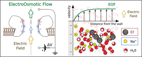
Micro and nanofluidic systems are intrinsically inhomogeneous due to the presence of confining walls, and, in many applications, the fluid is a liquid solution containing neutral and charged chemical species. The inhomogeneities due to wall geometry, chemical composition and charge affect the concentration of all the dissolved species, potentially inducing local charge accumulation even in a globally neutral fluid. An electroosmotic flow (EOF) arises when an external electric field acts on such an inhomogeneous system, e.g. when a voltage drop $\mathrm{\Delta }V$ is applied at the two ends of a pore. The electric field exerts a net force on the charged portions of fluid that, in turn, sets the fluid in motion.

A pictorial view of the simplest possible system in which electroosmosis occurs is sketched in Figure 1a. Consider an ionic solution in contact with a planar wall. The electric potential of the wall’s surface, with respect to the bulk fluid potential, termed henceforth the $\zeta$-potential, induces inhomogeneity in the system. For simplicity, we assume here that the solution is globally neutral far from the wall, with only two ionic species (anions and cations) with equal valency and bulk concentration $c_0$. This is a quite common situation, easily accessible experimentally, for instance dissolving a salt such as KCl in water. Due to electrostatic interactions with the wall, local electroneutrality will be broken in the near wall region and ions will be repelled by or attracted to the wall depending on their charge. Ionic diffusion balances this repulsion/attraction and tends to homogenize ion concentrations, see Figure 1a. This competition results in ionic accumulation/depletion peaked over a thin layer near the wall, referred to here as Debye layer.¹

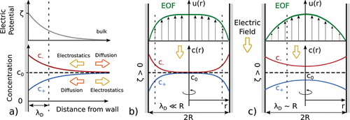
Figure 1. Electroosmosis working principle. a) Ionic density profiles $c_{+}$ and $c_{-}$ close to a planar wall with given electric wall potential, $\zeta$. The $\zeta$-potential induces an accumulation or depletion of ions according to their charge (here positive ions are in blue and negative ions in red). The accumulation is larger near the wall, and decreases far from the wall with a characteristic length ${\lambda }_D$, known as the Debye length. As a consequence of the net charge close to the wall, the fluid may be set in motion by an external electric field parallel to the wall, as shown in b and c. b) Electroosmotic flow (EOF) in a nanopore (no-slip boundary condition) for non-overlapping Debye layers, pore radius $R$ large compared to the Debye length ${\lambda }_D$. c) EOF for overlapping Debye layers, $R\simeq {\lambda }_D$.

The balance between electrostatic interactions and diffusion has been quantified independently by Gouy and Chapman, at the onset of the 20th century [19,20]. In their framework, it is assumed that ion concentrations verify the Boltzmann distribution in which the only force acting on the ion is due to the local electric field. In combination with Poisson’s equation for electrostatics, a closed equation for the electric potential is obtained [4,18,21]. The Poisson-Boltzmann equation can be analytically solved for simple geometries, such as planar walls or channels, in its linearized form, which holds for sufficiently small $\zeta$-potentials, – as shown by Debye and Hückel in 1923 [18,22]. Within this limit, the decay of the electrostatic potential in the fluid is exponential, with a lengthscale equal to the Debye length, here given by

(1) ${\lambda }_D=\sqrt{\frac{{\epsilon }_0{\epsilon }_r{k}_{B}T}{q^2\sum _{\alpha }{c}_{\alpha }{Z}_{\alpha }^2}},$(1)

where $T$ is temperature, $k_B$ the Boltzmann constant, ${\epsilon }_0$ vacuum permittivity, ${\epsilon }_r$ relative permittivity, $q$ the elementary charge and $c_{\alpha }$ and $Z_{\alpha }$ are, respectively, the number concentration and valency of the ionic species $\alpha$ in solution, e.g. $Z_{\alpha }=+1$ for ${\mathrm{K}}^{+}$ and $Z_{\alpha }=-1$ for $\mathrm{C}{\mathrm{l}}^{-}$. The balance between electrostatic and diffusive effects is clear in Eq. (1)(1) ${\lambda }_D=\sqrt{\frac{{\epsilon }_0{\epsilon }_r{k}_{B}T}{q^2\sum _{\alpha }{c}_{\alpha }{Z}_{\alpha }^2}},$(1) . A broader ${\lambda }_D$ is obtained at high temperatures. In contrast, sharper ionic distributions are obtained when electrostatic interactions are enhanced, with higher valency and ion concentration, or lower relative permittivity. In typical nanopore applications [14,23–26], with KCl water solutions at $300$ K, ${\lambda }_D$ calculated from Eq. (1)(1) ${\lambda }_D=\sqrt{\frac{{\epsilon }_0{\epsilon }_r{k}_{B}T}{q^2\sum _{\alpha }{c}_{\alpha }{Z}_{\alpha }^2}},$(1) ranges from $0.3\mathrm{n}\mathrm{m}$ for $1M$ KCl to $10\mathrm{n}\mathrm{m}$ for $1mM$ KCl.

The relative scale of the Debye layer ${\lambda }_D$ compared with the radius $R$ of the pore controls the characteristics of the EOF. When ${\lambda }_D\ll R$, as in most micrometric systems, see Figure 1b, the ionic distribution and the electric potential reach their bulk values over most of the pore volume but in the Debye layers. This condition is usually referred to as non-overlapping Debye layers. When an electric field parallel to the channel axis is applied, the net force acts only on the thin charged layers near the wall, generating a plug-like velocity profile, see $u(r)$ in Figure 1b. In such microfluidic settings, with non-overlapping Debye layers, electroosmosis enables in particular electroosmotic pumping [27]. In nanopores, in contrast, the channel size is often comparable to the Debye length, ${\lambda }_D\sim R$, see Figure 1c. In this case, the ion concentrations do not reach $c_0$ in the center of the channel and a net charge is present in the entire pore volume (overlapping Debye layers). Accordingly, for overlapping Debye layers $c_0$ has to be interpreted as the concentration of the salt in a large reservoir in equilibrium with the confined system. Consequently, an external electric field will result in a volume force through the entire pore generating a velocity profile qualitatively similar to the parabolic Poiseuille profile due to a pressure gradient, see $u(r)$ in Figure 1c. For strongly overlapping Debye layers, recent theoretical results suggest that fluid charges may not be sufficient to balance surface charges, resulting in a breakdown of the electroneutrality condition [28,29]. Overlapping Debye layers are quite typical in biological nanopores where the pore diameter is of the order of a few nanometers [9,13,15,25], while solid state nanopores, whose size may range from subnamometer scale [30] to decades of nanometers [31–33], may fall in both overlapping and non-overlapping cases.

1.2. Three routes to charge accumulation at pore walls

Figure 2. Three routes to charge accumulation at pore walls. I. Fixed charges. a) Typical nanopore setup. Surface charges at the pore wall attract a cloud of counterions. A voltage drop $\mathrm{\Delta }V$ applied across the membrane containing the pore generates an electric current, mainly of the counterions, and sets the fluid in motion. b) Surface charges of a wild type (WtFraC) and engineered (ReFraC) transmembrane FraC protein, at neutral pH. In red and blue, acidic (negative) and basic (positive) surface residues. The negative constriction of the wild type (WtFraC, cation selective) is inverted into a positive one (ReFraC, anion selective) by a point mutation [14]. c) Polymer brush functionalized nanochannel. The charge of the coating polymer can be tuned by the solution pH [34]. II. Voltage gating. d) Polarization of the membrane surface is controlled by an embedded electrode, whose potential $\mathrm{\Delta }{\mathrm{V}}_{\mathrm{G}}$ is externally controlled. In this example $\mathrm{\Delta }{\mathrm{V}}_{\mathrm{G}}<0$ and $\mathrm{\Delta }\mathrm{V}>0$ for cation selectivity. e) Cross-sectional Transmission Electron Microscopy image of a solid state nanopore showing well-separated metal levels (TiN) approaching the edge of the nanopore [35]. f) Single-layer suspended graphene nanopore. A gating gold electrode has been patterned on graphene to control the electric potential of the graphene sheet [36]. III. Induced Charge. g) Charge accumulation and fluxes for two different geometries. The normal component of the electric field at the solid–liquid interface (pink ${\mathbf{E}}_{\mathbf{n}}$), generated by an external transmembrane voltage drop $\mathrm{\Delta }\mathrm{V}$, drives the formation of the Induced Debye Layer. The tangential component of the electric field at the wall, ${\mathbf{E}}_{\mathbf{t}}$, moves the accumulated charges. h) Continuum simulation results for a negatively charged truncated-conical nanopore [37], showing the distribution of the net charge concentration and corresponding electroosmotic velocity field at negative bias $\mathrm{\Delta }\mathrm{V}=-5\mathrm{V}$. i) Induced charge selectivity and EOF in an uncharged cylindrical nanopore [38], exploiting symmetry breaking due to a lateral cavity surrounding the nanopore. The simultaneous inversion of ionic selectivity and electric field direction causes a unidirectional parabolic EOF. Points refer to molecular dynamics simulations, the line to a theoretical prediction based on continuum arguments. Images adapted from: b. Huang et al. [14], c. Yameen et al. [34], e. Bai et al. [35], f. Cantley et al. [36], h. Yao et al. [37], i. Di Muccio et al. [38].

As a key ingredient for electroosmosis, different mechanisms have been exploited to control the electric potential at the pore walls and hence charge accumulation. Here, we present three methods commonly used in nanopore technology: fixed charges, voltage gating and induced charges.

Fixed charges

The most commonly used approach is based on the manipulation of fixed surface charges at the pore wall, see Figure 2.I. Fixed surface charges attract counterions in solution resulting in an intrinsic accumulation of net charge in the pore lumen. Fixed charges are naturally present both in biological and solid state nanopores, Figure 2a.

In biological pores, surface charges are due to acidic and basic titratable amino acids (containing carboxyl or amino functional groups) and they often result in complex surface charge patterns that may include both positive and negative patches, Figure 2b. The charge of these amino acids can be partially tuned by altering the pH to modify their protonation state [15,39,40]. Moreover, biological pores can be engineered with point mutations [14,40,41] that alter the amino acid sequence. Both strategies present challenges mainly associated with the capability of the biological pore to properly self-assemble into the lipid membrane and form a well-defined structure even under extreme pH conditions and after mutation of exposed amino acids. Nevertheless, some pores are remarkably robust. For instance, $\alpha$-Hemolysin forms stable pores from $\mathrm{p}\mathrm{H}2.8$ to $\mathrm{p}\mathrm{H}11$ [15,26,40] while in the constriction of the CsgG nanopore, the central amino acid (Asn-70) can be mutated in any other of the 19 standard proteinogenic amino acids [41] without altering the stability of the assembled nonameric channel.

Solid state nanopores usually present a more uniform surface charge than biological pores. The charge can be either positive (e.g. $\mathrm{A}{\mathrm{l}}_2{\mathrm{O}}_3,\mathrm{Z}\mathrm{n}\mathrm{O}$) or negative (e.g. $\mathrm{S}\mathrm{i}\mathrm{N},\mathrm{S}\mathrm{i}{\mathrm{O}}_2$) depending on the interfacial properties of the material and the fabrication process [10]. The charge can be tuned by changing the salt concentration [42,43] and also the pH [44,45]. For example, the surface charge of $\mathrm{S}\mathrm{i}\mathrm{N}$ nanopores ranges from $0.0027\mathrm{C}/{\mathrm{m}}^2$ at $\mathrm{p}\mathrm{H}1.2$ to $-0.2\mathrm{C}/{\mathrm{m}}^2$ at $\mathrm{p}\mathrm{H}11$ [43]. In addition, multiple-coating techniques are available to functionalize solid membranes and transfer to synthetic nanopores some properties of biological nanopores [46,47], including: deposition from gas phase, surfactant adsorption, physisorption, monolayer and layer-by-layer self-assembly, and silanization. The charge of the functional groups, see Figure 2c, can be further tuned by changing the pH, the electrolyte type and its concentration [24,34,48–50], allowing one to completely neutralize or invert the pristine pore charge and, hence, the EOF direction.

As a final comment, it is worth noting that a fixed surface charge is not the only way to achieve such a kind of intrinsic selectivity, i.e. an accumulation of positive or negative ions in the absence of any external perturbation. Indeed, intrinsic net charge accumulation in confined geometries even with a zero surface charge of the solid was observed in atomistic simulations [38,51]. In brief, in real electrolytes, an equilibrium charge layering spontaneously arises at the solid–liquid interface due to the different sizes and solvation energies of cations and anions. Moreover, the preferential orientation of water molecules at the walls results in net interfacial dipoles. The presence of interfacial dipoles generates an intrinsic polarization of the membrane, resulting in an effective surface potential.

Voltage gating²

A second approach to generate charge accumulation is to embed a gate electrode electrically connected to the membrane, Figure 2d. In that way, the $\zeta$-potential is actively modulated by controlling the voltage of the gate, $\mathrm{\Delta }{\mathrm{V}}_{\mathrm{G}}$ [53,54]. In essence, the strategy is similar to the MOSFETs electron/hole population regulation in silicon conductive channels used in electronics [55]. Gate electrodes are usually fabricated with thin metal films [35,56–58] (see, for example, the TiN metal layers in Figure 2e), conductive polymers [59] or single-layer graphene sheets [36] (Figure 2f). The strenuous fabrication process (including a sacrificial layer, bonding, high temperatures for the film deposition, electron beam lithography or atomic layer deposition) often limits the resolution of experimental designs to channels with diameters $10-100$ nm. However, 2D sub-nanometric fluidic confinement is possible with voltage-gated materials fabricated with multiple layers of packed, electrically conductive, nanosheets (such as graphene [60] and MXene [61]).

Induced charge

The third mechanism exploits the externally imposed voltage drop between the two compartments to also induce charge accumulation in the pore. Indeed when an electric field is applied, ions migrate towards or away from the membrane, and can, under certain conditions, generate a local accumulation of net charge [62]. This net charge is temporary and can be released when the voltage drop is removed. The region in which charge accumulates has a thickness of the order of the Debye length and it is named Induced Debye Layer, IDL [38,63,64]. If charge accumulates inside the pore region, the same electric field can also induce an EOF.

The origin of the charge accumulation in the IDL and thus of the EOF is related to the normal and tangential components of the local electric field at the membrane/liquid interface which, in turn, depend on the pore geometry and on the fluid and membrane permittivities. This can be seen considering the jump conditions derived from Gauss’s law and the fact that the electric field is irrotational for two materials with different dielectric properties

(2) $\left({\epsilon }_F{\mathit{E}}_F-{\epsilon }_M{\mathit{E}}_M\right)\cdot \hat{\mathit{n}}=q_w,$(2)

(3) $\left({\mathit{E}}_M-{\mathit{E}}_F\right)\times \hat{\mathit{n}}=0,$(3)

where ${\epsilon }_F$ and ${\epsilon }_M$ are the electric permittivities of the fluid and the membrane, ${\mathit{E}}_F$ and ${\mathit{E}}_M$ are the electric fields at the boundary, respectively, on the fluid and membrane side, $q_w$ is the surface charge and $\hat{\mathit{n}}$ is the outward normal to the membrane. The normal component of ${\mathit{E}}_F$ drives the formation of the IDL, see Figure 2g, left side. The tangential components of ${\mathit{E}}_F$ will move these accumulated charges along the channel wall, generating the EOF, usually called induced-charge electroosmosis (ICEO) [62]. It is worth noting that an asymmetry is needed to generate a net EOF, since a perfectly symmetric system would generate perfectly symmetric ion flows and no net charge accumulation in the pore, see the cylindrical pore example in Figure 2g, right side.

In a lumped-parameter model, it is possible to describe the membrane as a capacitor able to accumulate and release charge in response to the external voltage drop, $q_a=C\mathrm{\Delta }V$, with $q_a$ the local accumulated charge (IDL) and $C$ the local membrane capacitance, Figure 2g. Considering the simple case of a planar solid membrane of thickness $h$ which is immersed in an electrolyte solution, the capacitance per unit surface can be approximated by $C\simeq {\epsilon }_0{\epsilon }_M{h}^{-1}$ [38,63]. Induced charge accumulation hence becomes particularly noticeable at sharp corners and in tiny nanopores, where the thickness of the solid substrate becomes very small [37,38]. It is worth noting that the existence of a non-zero ${\mathit{E}}_M$, Eq.(2(2) $\left({\epsilon }_F{\mathit{E}}_F-{\epsilon }_M{\mathit{E}}_M\right)\cdot \hat{\mathit{n}}=q_w,$(2) ), is needed for the formation of the IDL [38,63], and hence simplified models that for ${\epsilon }_M\ll {\epsilon }_F$ neglect ${\mathbf{E}}_M$ are not able to describe IDL and ICEO.

Such nanoscale ICEO has recently been investigated numerically. As a first example, in Figure 2h single-polarity ions in the Debye layer and their counterions massively accumulate near the edge of a conical nanopore. This accumulation results in the formation of electroosmotic vortices [37]. Another example is reported in Figure 2i, where geometrical symmetry is broken by a surrounding cavity outside the pore and EOF is achieved in the absence of fixed charges ($q_w=0$). This approach induces ion selectivity without altering the pore shape, surface charge or chemistry and, consequently, opens new possibilities for more flexible designs of selective nanoporous membranes [38].

Finally, an intriguing and important feature of ICEO is that the induced flow depends quadratically on the applied voltage $\mathrm{\Delta }V$ [38,62]. Indeed, the EOF scales roughly as $q_a\mathrm{\Delta }V$, where $q_a$ is also proportional to $\mathrm{\Delta }V$. This quadratic dependence results in unidirectional EOF, i.e. the direction of the EOF is always the same, even when the applied voltage drop is inverted, see Figure 2i. Hence, a net fluid flow can be generated using both AC or DC fields.

1.3. Modeling and computational challenges

The diversity of contexts in which electroosmosis arises hints at the potential hardships to properly model such flows. Indeed, a reliable description of EOF is challenging for several reasons that we recapitulate below.

First, it requires to describe precisely numerous forces. In fact, it should model the hydrodynamic transport of the fluid and the ionic species dissolved therein, the electrostatic interactions among the different charged species and with the solid surfaces, the polarization of the membrane and the effect of external forcings. In addition, the presence of particles such as colloids or proteins, which typically present peculiar charge distributions, requires additional modeling of their interactions with the electrolyte solution.

A further challenge comes from the wide range of spatial and temporal scales that are relevant to the phenomenon. To illustrate the diversity of scales at play, we consider a typical nanoporous sensing device. A voltage drop $\mathrm{\Delta }V$ is applied between the two reservoirs, see Figure 2a, and we probe the role of electroosmosis for the capture of an analyte (e.g. a protein, a nucleic acid, a pollutant) by the pore. The pore constriction is usually of the order of a few nanometers. The applied voltage drop $\mathrm{\Delta }V$ results in a funnel-like electric field outside the pore, decaying slowly as $1/r^2$ with $r$ the distance to the pore [65,66]. The electric field is therefore considerable even decades of nanometers away from the pore entrance. A reliable model of the flow in this external capture region, on scales much broader than the nanoscale pore, is crucial to determine the motion of the analyte from the bulk to the pore entrance. Along with this diversity of spatial scales, very different time scales are at play. The motion of analytes needs to be resolved inside the constriction and is quite fast as it only occurs over a short spatial range. However, capture events need to be resolved over long time scales as they are usually rare events.

Finally, as the system is usually extremely confined – such as in nanopores – thermal fluctuations have to be taken into account. Thermal vibrations of the pore’s structure affect the motion of analytes [67,68]. The number of analytes within the pore is also strongly fluctuating, as there are only a few particles within at a time [69–71]. Moreover, the analyte undergoes Brownian motion, so the interest in not on the analysis of a single capture event, but on a statistical description of the capture [11,72,73].

There is no single computational method that is able to handle all the aforementioned physical features – variety of forces, space and time scales, and intrinsic fluctuations – with the currently available high performance computational resources. Selectivity for specific ionic species by the nanopore constriction is ruled by electrochemical interactions that occur at nanometer scales thus calling for an atomistic description [39,74,75], which is discussed in Section 3. However, computational requirements make atomistic models unsuited for the modeling of the capture region, and, more importantly, prevent the implementation of efficient, computer-assisted, design strategies that usually require the exploration of a wide number of different operating conditions. Indeed, even on supercomputers, atomistic simulations hardly reach a microsecond/day, while typical capture and translocation time scales range from milliseconds to seconds [13,15,76,77]. Standard continuum models, discussed in Section 2, are computationally less demanding and they enable the description of long time scales but, on the one hand, they often require ad hoc nanoscale corrections, and, on the other hand, they do not include thermal fluctuations. Mesoscale models, discussed in Section 4, attempt to bridge the gap between continuum and atomistic descriptions, but often require external information (e.g. coarse-grained modeling of chemical interactions) that may need to be finely tuned to obtain quantitative results. In the following, we briefly review these different approaches with the aim to help researchers select the technique that better reflects the levels of accuracy and approximations suitable to answer a specific question. Finally, some of the most challenging applications related to EOF in nanopores are reported in Section 5.

2. Continuum methods

We start by reviewing how continuum models may be used to explore EOF, including a careful explanation of specific modeling assumptions that have to be made. We discuss representative examples. Finally, we explore the limitations of such continuum approaches.

Continuum models rely on a set of equations: the continuity equation for each species, the momentum and mass balance for the fluid, and the Poisson equation for electrostatics,

(4) $\frac{\mathrm{\partial }{c}_{\alpha }}{\mathrm{\partial }t}+\text{bnabla}\cdot \left(c_{\alpha }\mathit{u}+j_{\alpha }\right)=0,$(4)

(5) $\rho \frac{\mathrm{\partial }\mathit{u}}{\mathrm{\partial }t}+\rho \mathit{u}\cdot \text{bnabla}\mathit{u}\mathbf{=}\text{bnabla}\cdot \text{r}\mathbf{\Sigma }\mathbf{-}{\rho }_{\mathrm{e}}\text{bnabla}\mathbf{\Phi }\mathbf{,}$(5)

(6) $\text{bnabla}\cdot \mathit{u}=0,$(6)

(7) $\text{bnabla}\cdot \left(\epsilon \text{bnabla}\mathbf{\Phi }\right)\mathbf{=}\mathbf{-}{\rho }_{\mathrm{e}}\mathbf{,}$(7)

whose derivation can be found in standard microfluidics textbooks [4,18]. For each dissolved species $\alpha$, Eq. (4)(4) $\frac{\mathrm{\partial }{c}_{\alpha }}{\mathrm{\partial }t}+\text{bnabla}\cdot \left(c_{\alpha }\mathit{u}+j_{\alpha }\right)=0,$(4) describes the time evolution of the number density $c_{\alpha }$. The flux has two contributions, a convective flux $c_{\alpha }\mathit{u}$, where $\mathit{u}$ is the fluid velocity, and a nonconvective flux ${\mathbf{j}}_{\alpha }$ which has to be specified via a constitutive relation. Eq. (5)(5) $\rho \frac{\mathrm{\partial }\mathit{u}}{\mathrm{\partial }t}+\rho \mathit{u}\cdot \text{bnabla}\mathit{u}\mathbf{=}\text{bnabla}\cdot \text{r}\mathbf{\Sigma }\mathbf{-}{\rho }_{\mathrm{e}}\text{bnabla}\mathbf{\Phi }\mathbf{,}$(5) -(6(6) $\text{bnabla}\cdot \mathit{u}=0,$(6) ) describe momentum and mass balance of an incompressible flow. Here, $\rho$ is the (constant) fluid density, $\mathbf{\Sigma }$ is the stress tensor to be specified by a constitutive relation, $\mathrm{\Phi }$ is the electrostatic potential and ${\rho }_e$ is electric charge density, which is expressed in terms of the ionic species concentration $c_{\alpha }$ by

${\rho }_e=\sum _{\alpha =1}^{N_s}{c}_{\alpha }q{Z}_{\alpha },$

where $N_s$ is the total number of ionic species, $q{Z}_{\alpha }$ is the charge of species $\alpha$. Most fluids relevant to EOF are Newtonian fluids, for which the stress tensor reads

(8) $\mathbf{\Sigma }=-p\mathit{I}+\mathit{2}\eta \sigma ,$(8)

where $p$ is the pressure field, $\mathit{I}$ is the identity tensor, $\eta$ is the viscosity of the fluid and $\mathit{\sigma }=(\text{bnabla}\mathit{u}+{\left(\text{bnabla}\mathit{u}\right)}^T)/$2 is the strain rate tensor. When Eq. (8)(8) $\mathbf{\Sigma }=-p\mathit{I}+\mathit{2}\eta \sigma ,$(8) is used, the momentum and mass balance, Eq. (5(5) $\rho \frac{\mathrm{\partial }\mathit{u}}{\mathrm{\partial }t}+\rho \mathit{u}\cdot \text{bnabla}\mathit{u}\mathbf{=}\text{bnabla}\cdot \text{r}\mathbf{\Sigma }\mathbf{-}{\rho }_{\mathrm{e}}\text{bnabla}\mathbf{\Phi }\mathbf{,}$(5) –6(6) $\text{bnabla}\cdot \mathit{u}=0,$(6) ), are referred to as the Navier-Stokes equations. Complex fluids require more specific constitutive relations instead of Eq. (8(8) $\mathbf{\Sigma }=-p\mathit{I}+\mathit{2}\eta \sigma ,$(8) ), see, e.g. [78], where EOF in viscoelastic fluids is discussed. At sufficiently small scales, typical of nanopores, inertial and nonlinear terms, i.e. the left hand side of Eq. (5(5) $\rho \frac{\mathrm{\partial }\mathit{u}}{\mathrm{\partial }t}+\rho \mathit{u}\cdot \text{bnabla}\mathit{u}\mathbf{=}\text{bnabla}\cdot \text{r}\mathbf{\Sigma }\mathbf{-}{\rho }_{\mathrm{e}}\text{bnabla}\mathbf{\Phi }\mathbf{,}$(5) ), may usually be neglected,³ leading to the Stokes equation [79]. In the Navier-Stokes equations, Eq. (5)(5) $\rho \frac{\mathrm{\partial }\mathit{u}}{\mathrm{\partial }t}+\rho \mathit{u}\cdot \text{bnabla}\mathit{u}\mathbf{=}\text{bnabla}\cdot \text{r}\mathbf{\Sigma }\mathbf{-}{\rho }_{\mathrm{e}}\text{bnabla}\mathbf{\Phi }\mathbf{,}$(5) the term $-{\rho }_e\text{bnabla}\mathrm{\Phi }$ is crucial for the description of EOF: it drives solvent flow where charge is accumulated. Finally, Eq. (7)(7) $\text{bnabla}\cdot \left(\epsilon \text{bnabla}\mathbf{\Phi }\right)\mathbf{=}\mathbf{-}{\rho }_{\mathrm{e}}\mathbf{,}$(7) is the Poisson equation, derived from Gauss’s law in a medium of permittivity $\epsilon ={\epsilon }_0{\epsilon }_r$. The set of equations (4(4) $\frac{\mathrm{\partial }{c}_{\alpha }}{\mathrm{\partial }t}+\text{bnabla}\cdot \left(c_{\alpha }\mathit{u}+j_{\alpha }\right)=0,$(4) –7(7) $\text{bnabla}\cdot \left(\epsilon \text{bnabla}\mathbf{\Phi }\right)\mathbf{=}\mathbf{-}{\rho }_{\mathrm{e}}\mathbf{,}$(7) ) is closed once the flux of ionic species ${\mathit{j}}_{\alpha }$ is specified. Within linear response, considering standard Fickian diffusion and electrophoretic motion of the ions

(9) ${\mathit{j}}_{\alpha }=-D_{\alpha }\left(\text{bnabla}{c}_{\alpha }+c_{\alpha }\frac{q{Z}_{\alpha }}{k_{B}T}\text{bnabla}\mathrm{\Phi }\right),$(9)

Eq. (4)(4) $\frac{\mathrm{\partial }{c}_{\alpha }}{\mathrm{\partial }t}+\text{bnabla}\cdot \left(c_{\alpha }\mathit{u}+j_{\alpha }\right)=0,$(4) becomes the Nernst-Planck equation, which is widely used in the EOF literature. Eq. (9)(9) ${\mathit{j}}_{\alpha }=-D_{\alpha }\left(\text{bnabla}{c}_{\alpha }+c_{\alpha }\frac{q{Z}_{\alpha }}{k_{B}T}\text{bnabla}\mathrm{\Phi }\right),$(9) embeds several assumptions on the nature of the solution, which are briefly discussed in section 2.3.

The set of Eq. (4(4) $\frac{\mathrm{\partial }{c}_{\alpha }}{\mathrm{\partial }t}+\text{bnabla}\cdot \left(c_{\alpha }\mathit{u}+j_{\alpha }\right)=0,$(4) –7(7) $\text{bnabla}\cdot \left(\epsilon \text{bnabla}\mathbf{\Phi }\right)\mathbf{=}\mathbf{-}{\rho }_{\mathrm{e}}\mathbf{,}$(7) ) for a Newtonian fluid Eq. (8)(8) $\mathbf{\Sigma }=-p\mathit{I}+\mathit{2}\eta \sigma ,$(8) and a standard flux given by Eq. (9)(9) ${\mathit{j}}_{\alpha }=-D_{\alpha }\left(\text{bnabla}{c}_{\alpha }+c_{\alpha }\frac{q{Z}_{\alpha }}{k_{B}T}\text{bnabla}\mathrm{\Phi }\right),$(9) are known as the Poisson-Nernst-Planck-Navier-Stokes equations (PNP-NS), and, once proper boundary conditions are imposed, can be solved self-consistently via computational methods such as finite elements (FEM) or finite volumes (FVM) [80,81].

2.1. Boundary conditions

When modeling EOF in nanopores, care should be given to the selection of boundary conditions. It is convenient to divide boundaries into two groups: reservoir boundaries and membrane boundaries. In general, the domains on which the Poisson equation and the transport equations are solved differ. Transport equations are solved only in the fluid domain while the Poisson equation needs to be solved both in the fluid and in the membrane, in particular when the electric field inside the membrane is relevant, as is the case for induced charged EOF as discussed in section 1.2, see Figure 2 III.

Transport equations

For the ionic transport equations, it is reasonable to consider that far from the pore at both sides two reservoirs are present, each with a fixed concentration. This translates to the condition $c_{\alpha }=n_{\alpha ,1}$ and $c_{\alpha }=n_{\alpha ,2}$ at the boundary separating the system from the two reservoirs. If the ions cannot penetrate the membrane the impermeability condition $\hat{\mathit{n}}\cdot {\mathit{j}}_{\alpha }=0$ holds at the fluid-membrane interface, where $\hat{\mathit{n}}$ is the outward normal to the membrane surface, see e.g. Figure 3a (top). For what concerns fluid transport, usually it can be assumed that no mechanically induced flow is present. In this case, a zero stress condition can be used at the reservoir boundary $\hat{\mathit{n}}\cdot \mathbf{\Sigma }=0$. In the case of pressure-driven flow, the pressure at the inflow and outflow boundaries needs to be specified [82]. As for the fluid-membrane interface, the impermeability condition applies to the normal component of the velocity $\mathit{u}\cdot \hat{\mathit{n}}=0$. The boundary condition for the tangential component of the velocity requires some assumptions on the nature of the fluid-membrane interactions. If these are such that the fluid in contact with the membrane has zero velocity, a no-slip condition $\mathit{u}=0$ has to be used. However, especially inside the nanopore, the no-slip condition may fail to represent the fluid-membrane interaction and can be substituted by the more general Navier slip condition, in which the stress exerted by the membrane on the fluid is proportional to the velocity of the fluid at the interface [83,84]. $\left(2b\hat{\mathit{n}}\cdot \sigma -\mathit{u}\right)\cdot \left(\mathit{I}-\hat{\mathit{n}}\otimes \hat{\mathit{n}}\right)=0$ (where $b$ is usually a scalar except for anisotropic surfaces [85]). The slip length $b$ is a parameter, which quantifies the motion of the fluid with respect to the wall at the boundary [86] and characterizes the liquid/solid interactions. For example, slippage increases with hydrophobicity [87–89]. In practical cases of hydrophilic or slightly hydrophobic membranes, $b$ is usually in the nanometer range, and is therefore mostly relevant in the pore. Yet, even a subnanometer slip length may strongly affect the EOF intensity [90].

Poisson’s equation

The membrane and the fluid have in general different dielectric properties and often a surface charge $q_w$ is present at the fluid-membrane interface. Hence, the electric field can be discontinuous at the interface. This requires to solve Poisson’s equation separately in two subdomains, the fluid and the membrane subdomains, introducing an internal boundary (i.e. the fluid-membrane interface where a matching condition should be imposed) and an external boundary (i.e. the whole domain boundary). At the interface between the fluid subdomain and the reservoirs, a voltage drop can be imposed by setting $\mathrm{\Phi }=0$ at one reservoir and $\mathbf{\Phi }\mathbf{=}\mathrm{\Delta }V$ at the other, see Figure 3a. At the external boundary of the membrane, a vanishing normal component of the electric field can be used ($\hat{\mathit{n}}\cdot \mathbf{E}=0$) – assuming that the domain is sufficiently large to consider the nanopore far enough, see the small brown external boundary of the membrane in Figure 3a. For the internal boundary, the appropriate equations are given by the already mentioned jump conditions derived from Gauss’s law and the irrotationality of the electric field, see Eq. (2(2) $\left({\epsilon }_F{\mathit{E}}_F-{\epsilon }_M{\mathit{E}}_M\right)\cdot \hat{\mathit{n}}=q_w,$(2) –3(3) $\left({\mathit{E}}_M-{\mathit{E}}_F\right)\times \hat{\mathit{n}}=0,$(3) ). A surface charge in the membrane can be represented either by explicitly setting $q_w$ in the jump condition of Eq. (2)(2) $\left({\epsilon }_F{\mathit{E}}_F-{\epsilon }_M{\mathit{E}}_M\right)\cdot \hat{\mathit{n}}=q_w,$(2) or by adopting a sufficiently thin slice of volumetric charge density inside the membrane close to its surface, as for instance in [91].

2.2. PNP-NS model to study electroosmotic flows

The PNP-NS model has been widely used to model EOF. Under the Debye-Hückel approximation (i.e. small $\zeta$-potential), the set of Eq. (4(4) $\frac{\mathrm{\partial }{c}_{\alpha }}{\mathrm{\partial }t}+\text{bnabla}\cdot \left(c_{\alpha }\mathit{u}+j_{\alpha }\right)=0,$(4) –7(7) $\text{bnabla}\cdot \left(\epsilon \text{bnabla}\mathbf{\Phi }\right)\mathbf{=}\mathbf{-}{\rho }_{\mathrm{e}}\mathbf{,}$(7) ) can be solved with semi-analytical perturbative approaches in case of channels of smoothly varying section and sufficiently low external voltages. These approaches have been used to capture important qualitative features, such as the presence of recirculating regions in which the flow direction is opposite as compared to the average volume flow [92], as confirmed also via molecular dynamics simulations [93]. These approaches can also be used to characterize the linear response of such channels in terms of fluxes (electric, concentration and mass) under different external stimuli [94].

In the case of high $\zeta$-potentials and external fields, the solution of Eq. (4(4) $\frac{\mathrm{\partial }{c}_{\alpha }}{\mathrm{\partial }t}+\text{bnabla}\cdot \left(c_{\alpha }\mathit{u}+j_{\alpha }\right)=0,$(4) –7(7) $\text{bnabla}\cdot \left(\epsilon \text{bnabla}\mathbf{\Phi }\right)\mathbf{=}\mathbf{-}{\rho }_{\mathrm{e}}\mathbf{,}$(7) ) may quantitatively differ from the one obtained with linearized approaches. Moreover, when the channel section varies abruptly, as in many nanopore applications, such approaches may fail to properly describe the ionic distributions [92]. In these cases, the numerical solution of the complete non-linear PNP-NS system may be required. For example, Melnikov et al. [91], showed that, even for simple systems such as charged cylindrical nanopores, finite pore length leads to substantial differences with respect to analytic results regarding infinitely long channels of constant section. The velocity field of the nonlinear PNP-NS for a charged finite cylinder for two different pore radii is reported in (Figure 3(b,c)), left side. The axial velocity profiles inside the pore (full lines) are compared with analytic predictions for infinite cylinders (dashed and dotted) in (Figure 3(b,c)), right side. The PNP-NS solution differs quantitatively from the analytic result, especially for shorter pores. This can be ascribed to the assumption of an infinite channel length that neglects pore entrance effects.

Furthermore, interesting qualitative features of the velocity profile inside pores may be revealed with continuum models – and differ from analytic predictions for infinitely long cylinders (Figure 3(b,c)). Due to the fluid incompressibility, a pressure difference builds up between the two ends of the pore. This pressure drop generates a force density that opposes the electroosmotic flow. If the pore is sufficiently short, this force density may overcome the electrostatic force density contribution, inducing a change in the concavity of the velocity profile. Since the electroosmotic driving force is mainly located in the Debye layer, this effect depends on the ratio of the Debye length ${\lambda }_D$ to the pore radius. With a short Debye length with respect to the pore radius, the flow is surface-driven and hence the force density generated by the pressure drop induces a relative minimum at the center of the pore, where the electrostatic contribution vanishes. In a system in which the Debye length is comparable to the pore radius, the flow is bulk-driven and the force density induced by the pressure drop is counterbalanced by the electrostatic force density, now relevant also in the center of the pore, resulting in a maximum of the velocity profile at the center [91].

Figure 3. Examples of EOF solved within the PNP-NS framework. Panels a and d are adapted from Willems et al. [25], while panels b and c are adapted from Melnikov et al. [91]. Boundary conditions. a) Model for a typical nanopore geometry with the different components of the PNP-NS equations and boundary conditions. Here, dielectric constant $\epsilon$, viscosity $\eta$, diffusivity $D$ and fluid density $\rho$ depend on the local ion concentration, while $\eta$ and $D$ also depend on the distance to the solid boundary. Effect of pore size. b) Velocity field and axial velocity profile inside a cylindrical nanopore with radius $5$ nm. The surface charge of the membrane and the voltage drop $\mathrm{\Delta }V$ applied via boundary conditions give rise to EOF. Solid lines on the velocity profile represent the result of PNP-NS numerical simulations, while dashed and dotted lines show the analytical solution for the linearized Debye-Hückel theory for an infinitely long pore, using two different expressions for the $\zeta$-potential. c) Same as b), considering a nanopore with larger radius, $10$ nm. Effect of concentration. d) Electroosmotic velocity field inside a biological nanopore (ClyA) and axial velocity profile at the constriction. The biological nanopore is modeled as a fixed spatial charge density. The geometry of the nanopore, extracted from its molecular structure, is used as a boundary for the fluid domain. The velocity profile is shown for different ion concentrations (hence, different ${\lambda }_D$).

More complex pores have also been explored by continuum methods. Biological nanopores have an extremely complex geometry and charge distribution, which makes them difficult to simulate in a continuum framework. Still, continuum models of biological pores can be built and investigatedfor example, Willems et al. [25] investigated a continuum model for the geometry and charge of Cytolysin A (ClyA), see Figure 3d, a toxic protein produced by E. Coli. An extended PNP-NS approach in which steric effects have been added to the constitutive relation Eq. (9)(9) ${\mathit{j}}_{\alpha }=-D_{\alpha }\left(\text{bnabla}{c}_{\alpha }+c_{\alpha }\frac{q{Z}_{\alpha }}{k_{B}T}\text{bnabla}\mathrm{\Phi }\right),$(9) for the ionic flux [95] was used to study the transport of ions and water through the pore. Properties such as ionic mobilities, electric permittivity, fluid density and viscosity were modeled as dependent on the local ionic concentration and on the distance to the liquid-solid interface, see Figure 3a (bottom). The resulting velocity field is shown in Figure 3d (left side), with axial velocity profiles computed at the pore constriction for different salt concentrations shown in Figure 3d (right side). Interestingly, the change in the velocity profile with increasing salt concentration (and hence decreasing Debye length ${\lambda }_D$) shows a minimum in the center of the pore similar to the one observed for cylindrical channels, see Figure 3c. This suggests both that finite pore length effects are important in biological pores, and that a key role is played by the ratio between ${\lambda }_D$ and the pore size in determining the presence of such effects.

In addition to the aforementioned examples, the PNP-NS model has been widely used to study several systems and setups such as induced charge electroosmosis [37,96], EOF rectification [97], EOF reversal in a glass nanopore [98] and the effect of EOF on ionic current rectification [99]. In all these cases, nonlinear effects due to charge redistribution under the applied voltage are crucial, and cannot be captured by analytical approaches based on the linearized Poisson-Boltzmann equation. As previously reported, semi-analytical perturbative approaches [92,94] may be used to study EOF in smoothly varying channels. Such semi-analytical approaches are much more computationally efficient when compared to PNP-NS and can therefore prove useful when a fast screening of the EOF in several operating conditions is needed, e.g. for design purposes. Similarly, analytical models for the electric conductance including also the effect of liquid slippage at the wall [7,100], and EOF models for finite cylindrical pores [101] have been developed. Although these models are often limited to simplified geometries (e.g. cylindrical pores), they can still provide preliminary indication of the magnitude of the currents.

2.3. Some limitations of the PNP-NS model

Despite the complexity and variety of systems that can be studied, the PNP-NS model suffers from some limitations, and requires variations or entirely different approaches to tackle specific problems. We explore three major limitations below.

Electrolyte model

The PNP-NS equations rely on a model for the ion flux, Eq. (9(9) ${\mathit{j}}_{\alpha }=-D_{\alpha }\left(\text{bnabla}{c}_{\alpha }+c_{\alpha }\frac{q{Z}_{\alpha }}{k_{B}T}\text{bnabla}\mathrm{\Phi }\right),$(9) ), which is based on several assumptions. In particular, the chemical potential of the solvent is not taken into account, while the chemical potential for solutes is assumed to be well described by an ideal (dilute) solution approximation, ${\mu }_{\alpha }=k_{B}Tln\left(c_{\alpha }/c_0\right)+Z_{\alpha }q\mathrm{\Phi }+{\tilde{\mu }}_{\alpha }$, where $c_0$ is a reference concentration, and ${\tilde{\mu }}_{\alpha }$ is a constant. Eq. (9)(9) ${\mathit{j}}_{\alpha }=-D_{\alpha }\left(\text{bnabla}{c}_{\alpha }+c_{\alpha }\frac{q{Z}_{\alpha }}{k_{B}T}\text{bnabla}\mathrm{\Phi }\right),$(9) also assumes a diagonal diffusivity, meaning that the motion of the different species is uncorrelated. For a detailed discussion of other underlying assumptions, we refer the reader to Dreyer et al. [102]. All these assumptions limit the scope of the results. For example, at high concentrations the dilute approximation breaks down and an alternative model for the chemical potential has to be used [103]. More complex models for the chemical potential can be formulated to obtain expressions for the flux, which take into account specific features of the solution, such as steric and solvation effects [104–109]. Taking into account steric effects leads to reduced charge accumulation near the charged surfaces, mitigating the highly nonlinear effects arising when high $\zeta$-potentials are involved [110,111]. This overestimation of the charge density may significantly affect the predicted EOF [112].

Confinement

Beyond modeling assumptions for the bulk electrolyte, when dealing with nanopores, the behavior of the solution is dramatically affected by the extreme confinement in the pore region. In fact, from a few tens of nanometers and below, the growing importance of surfaces triggers a diversity of surprising effects, challenging the continuous description of hydrodynamics Eq. (5(5) $\rho \frac{\mathrm{\partial }\mathit{u}}{\mathrm{\partial }t}+\rho \mathit{u}\cdot \text{bnabla}\mathit{u}\mathbf{=}\text{bnabla}\cdot \text{r}\mathbf{\Sigma }\mathbf{-}{\rho }_{\mathrm{e}}\text{bnabla}\mathbf{\Phi }\mathbf{,}$(5) –6(6) $\text{bnabla}\cdot \mathit{u}=0,$(6) ). First, water transport becomes strongly affected by the interactions with the pore wall material inducing an effective slip of water, discussed above, which can enhance the EOF [90]. Slippage at the interface may also be dependent on the structure of the confined ions, especially in subnanometer pores [113]. Furthermore, at subnanometer confinement water reorganizes in layers, strongly suppressing dielectric permittivity [114,115]. An effective dielectric permittivity may be used in Poisson’s equation Eq. (7(7) $\text{bnabla}\cdot \left(\epsilon \text{bnabla}\mathbf{\Phi }\right)\mathbf{=}\mathbf{-}{\rho }_{\mathrm{e}}\mathbf{,}$(7) ), see e.g [116]. The mobility of ions depends on their distance to the wall, which can be modeled by e.g. phenomenological diffusion coefficients for the ions [25]. Finally, the interplay between ionic and water transport at interfaces modifies currents: for example phenomena akin to passive voltage gating have been observed in confinements smaller than 2 nm, where ionic mobility under applied pressure depends on the applied voltage drop [113]. Naturally, it is expected that for similar osmotic-like transport, such as EOF, such curious coupling would also arise.

Such effects undoubtedly call for atomistic models that we discuss in section 3. Note that, at small confinements, standard atomistic models such as molecular dynamics, may still fail to reproduce quantitative agreement between measurements and simulations. In fact, electronic interactions are at play and only ab initio descriptions can provide accurate models [117,118].

Fluctuations

As a final remark, the PNP-NS model relies on a mean field approach, in which the fluctuations with respect to the average value of the fields (i.e. velocity, concentration, voltage, surface position) are not taken into account. Such fluctuations are present at all scales but their importance increases for the smallest nanopore systems [119–121]. The presence of thermal fluctuations affects the fluid velocity both directly due to thermal agitation of the solvent molecules, and indirectly, since fluctuations in the ionic distribution affect the driving electroosmotic force. Hence, continuum descriptions may fail to be either quantitatively or even qualitatively correct in very narrow nanopores. We refer the reader to Ref [122] for further insight on the breakdown of continuous equations in confinement.

3. Atomistic description

3.1. Challenges in the numerical implementation

Atomistic simulations have been widely used to study transport phenomena at the nanoscale [38,74,87,88,90,93,123–137]. The setup is straightforward: each atom is described as a classical material point of specified mass and charge. The material points interact via conservative forces and the system evolves in time according to Newton’s second law. In the literature, this approach is often referred to as all-atom Molecular Dynamics to be distinguished from coarse-grained methods [138–140] where material points do not necessarily correspond to single atoms. In the following, for simplicity we use Molecular Dynamics (MD) to refer to all-atom approaches.

The time evolution of such a mechanical system with $N$ particles in a limited volume $V$ interacting via conservative forces (such that the total energy $E$ is constant) corresponds to a thermodynamically isolated system, that samples the microcanonical ensemble (NVE). In practical applications, NVE systems are quite rare and, consequently, MD approaches were complemented by several, now standard, tools. Modifying the dynamics allows one to sample other statistical mechanical ensembles such as the canonical (NVT, with $T$ temperature) and the isobaric-isotermic (NPT, with $P$ pressure) ensembles. We refer the reader to classical resources [141–143] for more details. We focus here on three specific aspects that we believe to be especially relevant (and, in some cases, somewhat overlooked) to model EOF across nanopores, namely (i) what pore model is used, (ii) how to acknowledge for large reservoirs and especially how many particles to simulate within the pore in the absence of reservoirs and (iii) how to infer transport properties out of equilibrium (in the context of EOF when a voltage drop is applied).

i) Pore model: structure and interaction forces

For each pore investigated, in MD simulations its structure and the effective interaction forces between the pore atoms and the other species have to be specified . According to the type of pore under scrutiny (biological or artificial), modeling challenges are different.

A fundamental requirement for the simulation of a biological pore is the presence of a reliable experimentally determined structure (i.e. the conformation of the folded proteins constituting the pore). Macromolecular structures can be determined from protein crystals using a variety of methods, including X-Ray Diffraction/X-ray crystallography [144], Cryogenic Electron Microscopy [145] (CryoEM), Small-angle X-ray scattering [146] and Neutron diffraction [147]. Those structures are typically accessible on the Protein Data Bank (PDB [148]), while dedicated databases, such as OPM [149] and MemProtMD [150], provide spatial arrangements of proteins with respect to the lipid bilayer membrane, largely facilitating the simulation setup. Several well-characterized structures are nowadays available, such as the widely studied $\alpha$ -Hemolysin ($\alpha$-HL[151]), FraC [152] (see also Figure 2-I.b) and Mspa [153].

If the structure is not available, or if it is only partially available, different protein modeling softwares such as Swiss-Model [154] or MODELLER [155] can be used to get a complete structure. When the protein portion to be modeled is located towards the pore lumen or at the pore entrances, in general such strategies do not guarantee reliable assessment of ion transport properties (such as selectivity) or EOF. In fact, a slight inaccuracy in the determination of the protein structure could result in a significant modification of the nanoscale confinement. Only in a few specific contexts is such modeling reliable: for example in CsgG [156] where the region to be modeled is small and on the exterior of the pore [38], or in the Aerolysin pore where the region to be modeled is a small portion of the extremely stable $\beta -$ barrel [157,158]. In both cases, MD simulations were set up using standard tools and resulted in stable structures. Finally, even if a complete structure is available, doubts may arise concerning the amino acid protonation state, in particular if the simulation pH is different from the physiological value. In that case, common strategies are to use dedicated bioinformatics tools, such as H++ [159] or PROPKA [160] to predict the acid dissociation constant ${\mathrm{K}}_{\mathrm{a}}$ for each titratable residue. ${\mathrm{K}}_{\mathrm{a}}$ is then used to calculate the protonation state [14,15,26,39].

In the last decades, reliable atomistic models for the interaction forces among atoms of biological molecules (such as proteins, DNA, lipids) have been developed [161,162]. These models, often referred to as force fields in the MD jargon, are typically used for the simulation of transport phenomena through biological membranes [74,124,163–165]. For solid state pores, while the structure is inferred by design, the reliability of force-fields is less clear. This is in part due to the diversity of experimental fabrication techniques and material properties for solid-state pores (metallic, non-metallic, semi-conducting) that makes force-field calibrations more challenging. Specifically, although classical force fields for common membrane materials are widely used (such as for $\mathrm{S}{\mathrm{i}}_3{\mathrm{N}}_4$ [125], carbon nanotubes [126,127] graphene [128,129] and $\mathrm{M}\mathrm{o}{\mathrm{S}}_2$ [130,131]), open issues arise concerning their surface charge and their effective dielectric constant. In particular, the determination of the surface charge for solid state pores as a function of the properties of the electrolyte solution is per se an open issue [29]. Force-fields may however at least be calibrated to reproduce wetting properties (to account properly for fluid-solid interactions) and mechanical properties (to properly reproduce thermal vibrations) [166].

Nevertheless, simulations of solid state pores may be very useful in electroosmosis research since solid state structures are perfectly suited to set up somehow ideal simulations aimed at discovering general trends in EOF. Examples are the analysis of the role of electric field intensity in EOF through a graphene nanopore [132], the role of local electroneutrality breakdown [29] and eddy formation due to EOF in varying-section channels [93] and the proof of principle of induced charge selectivity in cylindrical neutral channel discussed in Figure 2-III [38]. More generally, MD simulations in simple solid state geometries may be used to assess the validity limit of continuum PNP-NS theories and to determine peculiar nanoscale effects [133].

ii) Number of molecules within the pore: modeling the effect of reservoirs

The number of molecules within the nanopore is a highly dependent function of the system properties. In most experimental settings, the aqueous solution within the pore is always in contact with a large reservoir where it is possible to control bulk macroscopic conditions, such as temperature $T$, pressure $P$ and salt concentration $c$. At equilibrium, the number of molecules that occupy the pore is ruled by chemical potential equilibrium between the bulk and pore regions. For pores of size $R$ much larger than the Debye length ${\lambda }_D$ and the molecule size $a$, typically bulk conditions are reproduced inside the pore. The number of molecules can be reliably approximated as the pore volume times the bulk concentration of each single species. However, this is not the case for narrow pores where $L\simeq {\lambda }_D$ or $L\simeq a$. For example, a positively charged narrow pore will typically contain more negative ions than positive ions. The number of ions inside the channel is a fluctuating quantity in time [69,71]. Surface hydrophobicity also plays a role in determining the appropriate average water density. In the case of highly hydrophobic patches, even the mere presence of the electrolyte solution inside the pore is questionable since vapor bubbles may form [167–169]. In MD simulations, however, the total number of atoms of each species is generally kept constant throughout the simulation. Hence, specific strategies are required to ensure that the number of atoms chosen is compatible with the corresponding real system.

The standard way to tackle this issue in nanopore systems is to explicitly simulate reservoirs on the two sides of the pore. This approach allows one to directly use standard tools present in common MD packages [170–172] (e.g. flexible cell barostats) that, when employed during the equilibration, adapt the box size independently in the three directions. Details of this method can be found, among others, in [74,129,136]. This solution requires to dedicate a relevant part of the computational resources to the modeling of the reservoirs. It is therefore useful to find alternative approaches.

To avoid reservoirs, one approach is to impose periodicity along the pore axis. This is especially suited for long pores, where entrance effects are not dominant, and reservoirs have a limited impact on ionic and electroosmotic flow. This can be done, for instance, to investigate flows in a long nanotube [134] or in a planar channel [133,135] and to disentangle entrance effects. Thus, this approach is not applicable to biopores that are typically short and in which entrance effects are crucial, especially due to asymmetric pore entrances. When employing this strategy, care should be taken to select the number of atoms constituting the confined electrolyte solution. This is important for example to avoid bubble formation. In planar geometries, this is easily circumvented by either imposing a mechanical pressure on the walls [137,173], using a barostat along the direction normal to the walls [87,88] or anchoring the wall atoms to a spring and calibrating the constraint position to get the prescribed pressure [174]. The extension of these methods to cylindrical geometries is not straightforward and, to the best of our knowledge, never reported in the literature. Careful choice of the number of confined atoms is also essential to ensure that the local chemical potential is in equilibrium with that of the (non-simulated) reservoirs. For example, Widom’s insertion method [175] can be used to estimate the chemical potential and adapt the number of molecules in nanochannels [176], though, to the best of our knowledge, such an approach has not yet been conducted in cylindrical geometries.

A few other, quite novel, approaches exist to remove reservoirs entirely yet mimick their effect. If the nanopore is sufficiently long,⁴ the nanopore alone can be simulated [116]. Typically, this requires to simulate the system with several values of the number of ions $N$ and to average transport properties for different $N$ with the grand canonical probabilities of having $N$ ions in the channel (related to the free energy). In contrast if the nanopore is short, fluctuating particle numbers have to be dynamically resolved. Inserting particles in the channel with effective rates depending on the geometry of the system does not reproduce correct statistical properties of the system in general [71,177]. Alternatively, simulation of two ‘line-like domains’ (one facing the pore and one for the rest of the reservoir) yields satisfactory results [71]. Such strategies are quite novel and require extensive care to be manipulated in different systems. However, they all represent promising routes to avoid explicit simulation of reservoirs.

In any case, proper account of the number of molecules within the pore is a crucial step. A possible consequence of a larger or lower number of solvent molecules or ions in the pore region, is the unrealistic representation of liquid layering at the wall. In particular, the effective thickness of the equivalent vacuum layer induced by the presence of the liquid–wall interface, referred to as the depletion layer [178], is directly related to liquid slippage at the wall [86,174], that, in turn, can strongly affect the EOF [90]. Another obvious consequence is the incorrect account of electrostatic interactions and thus of the accumulated charge.

iii) Accounting for heat fluxes in non-equilibrium simulations

The most common approach to infer transport properties is to perform non-equilibrium MD (NEMD) runs where an external forcing induces the flow of the solution [39,74,179,180]. The solid walls are constrained to the simulation box and do not move. The external forcing (external electric field in the case of EOF) results in a net work on the system. In experimental designs, systems are neither periodic nor isolated but they are in contact with a heat bath. Hence, the work done by the external forcing is converted into heat by viscous friction and eventually a heat flux from the system to the heat bath sets in. MD is typically run in periodic systems with no external boundaries (e.g. triperiodic systems). To reproduce heat flows in NEMD, the common strategy is to adapt the system’s equilibrium temperature control tools. These tools, indicated as thermostats, alter the dynamics: typically in $NVT$ simulations the total energy is not a conserved quantity but the average kinetic energy of the atoms is constrained. For a comprehensive introduction on thermostats see, among others [142,143]. When no net motion is present (as in equilibrium simulations) constraining the kinetic energy amounts to prescribing the temperature $T$. However, in NEMD, when a flow sets in, the kinetic energy of the atoms is not equally distributed among the three translational degrees of freedom; it is larger in the direction of the flow. As a consequence, the standard usage of thermostats on all the degrees of freedom may artificially modify ion and solvent flows.

Several solutions have been presented to limit possible artifacts. One route is to couple only the solid atoms to the thermostat [38,75]. Another possibility is to apply the thermostat only to the translational degrees of freedom orthogonal to the flow direction [181]. Note that this is possible only when studying periodic pores where no EOF funneling at the pore entrance is present. Finally, in some cases, the kinetic energy associated with the streaming velocity is a very small fraction of the total kinetic energy [133,135]. Hence, the application of a standard thermostat that acts on all the three translational degrees of freedom is expected to be satisfactory to infer transport coefficients.

To infer transport coefficients, another possibility is to simulate equilibrium systems and use linear response theory. This so-called Green-Kubo approach has been employed extensively to study flows at the nanoscale [179,182,183]. The main advantage is that the system may be simulated at equilibrium and hence heat fluxes are entirely avoided. One common drawback, however, is that the method suffers from the so-called plateau problem, namely that the method requires infinitely long simulation times to converge, a problem that has only recently been solved [184]. Note that both NEMD and Green-Kubo approaches are equivalent in the linear regime [179].

Other aspects

Performing MD simulations of EOF in confined geometries encompasses other challenges beyond the three discussed previously. One additional relevant issue is the choice of the water and ion models. Indeed, 3 points water models do not quantitatively reproduce the viscosity and the diffusion coefficient of water. For quantitatively accurate predictions, one should rely on 4 points water models such as TIP4P/2005 [185,186]. However, standard force fields for biomolecules and ions are calibrated using 3-points water models [187]. Consequently, there is an inevitable balance between better acknowledgment of biomolecule–water interactions or water viscosity and diffusion. A similar problem occurs for ions. Standard rules for non-bonded interactions (Lorentz-Berthelot [142]) do not reproduce quantitatively correct ionic conductivities and ad hoc corrections to force fields have been recently proposed (e.g. CUFIX [188] correction for CHARMM [161]).

Another debated topic is how to apply the external forcing. In typical experimental conditions, a voltage drop $\mathrm{\Delta }V$ is applied between two reservoirs that are separated by the nanoporous membrane. The distance from the membrane to the electrode is typically orders of magnitude larger than the pore diameter and, hence, as a first approximation, the reservoirs can be considered infinite. On the other hand, fast computation of electrostatic interactions in MD simulations requires periodic boundary conditions [189] so, in essence, any simulated system is not a single pore but a series of arrays of pores. This is obviously incompatible with fixed voltage boundary conditions. The usual solution is to apply a constant and homogeneous electric field ($E$) parallel to the pore axis and wait for the migration of ions towards the membrane. It has been shown that this solution is equivalent to the application of a voltage drop $\mathrm{\Delta }V=L_{z}E$ where $L_z$ is the size of the periodic box in the axial direction [190].

Figure 4. Biological Nanopores. a) $\alpha$-Hemolysin ($\alpha$-HL) at different pH. Titratable residues in the interior surface affect the pore selectivity [26,39]. The positively and negatively charged residues are in blue and red, respectively. At low pH (left), the acidic residues are almost all protonated (neutral), and the pore interior is mainly positively charged. The pore is thus anion selective and an EOF sets in, in the direction opposite to the electric field. At high pH (right), acidic residues and tyrosines (pK_a $\sim$ 10.5) become negative, and some basic groups become neutral (histidines, N-terminals). Consequently, the overall $\alpha$-HL interior becomes neutral. and EOF vanishes. b) EOF from MD simulations for $\alpha$-HL in 1 M NaCl water solution for $\mathrm{\Delta }V=-125$ mV at different pH. Data for pH = 7 and pH = 10 are taken from [26]; data for pH = 2.8 and pH = 11 are original data obtained by using the same protocol, (protonation states predicted by H++ server [159]). c) DNA-origami nanopore. Cartoon representation (gray) of the initial (left) and equilibrated (right) DNA structure, overlaid with a chickenwire representation (colors). In the chickenwire representation, beads indicate the locations of the centers of mass of individual basepairs; horizontal connections between pairs of beads indicate interhelical crossovers. The lipid surrounding the DNA is sketched in grey, and the 1 M KCl water solution atoms filling the simulation box are not shown. d-f) Local density (gray scale) and local velocity (streamlines) of ${\mathrm{K}}^{+}$ (d) and $\mathrm{C}{\mathrm{l}}^{-}$ (e) ions and water (f) through the system of panel c at 400 mV. Panels c-f are adapted from Yoo and Aksimentiev [191].

3.2. Applications to study EOF in biological nanopores

Here, we report two examples of MD simulations of EOF in biological pores.

$\alpha$-Hemolysin

The most widely studied biological nanopore through MD is $\alpha$-Hemolysin ($\alpha$-HL), whose first simulation was reported by Aksimentiev and Schulten [74]. The pore was characterized in terms of permeability for water and ions at standard temperature and pressure. The system was composed by $\sim 300000$ atoms, including the protein, the lipid bilayer and a 1M KCl water solution. By applying an external electric field, an ionic current was established. The measured total current and ionic selectivity were in excellent agreement with available experimental data, demonstrating the capability of non-equilibrium MD simulations to predict with quantitative accuracy ionic currents through transmembrane biological pores induced by applied voltages. Afterwards, many studies were published using a similar all-atom setup to obtain molecular insight on current blockage due to macromolecules inside the pore (DNA, proteins) [165,192–194] and to study the effect of different salt types, concentration [75], or protonation state of the exposed residues [26,39] on ionic selectivity and EOF. At neutral pH, several charged residues (both positive and negative) are present in the pore interior and $\alpha$-HL is slightly anion selective. The charge of such residues can be altered by varying the pH of the solution, see Figure 4a. In particular, at low pH the pore interior is mostly positively charged, as aspartic acid and glutamic acid are almost all neutralized, whereas histidine, lysine and arginine have a positive charge. In such conditions, anions accumulate in the pore resulting in a strong unbalance of positive and negative ionic fluxes and an intense EOF, see Figure 4b. Conversely, at high pH, acidic residues and tyrosines (hydroxyl group, pK_a $\sim$ 10.5) become negatively charged, while some basic groups, such as histidines and N-terminals (pK_a $\sim$ 8.7) become neutral. The reduction of the net charges of the pore surface leads to a reduction of the pore selectivity and, consequently, the EOF is negligible, Figure 4b. This scenario is in fair agreement with experiments by Asandei et al. [15], where a positively charged peptide was captured in $\alpha$-HL against electrophoresis at pH = 2.8, while it is not captured at pH = 7, in agreement with EOF strengthening at low pH.

DNA-origami nanopore

Another interesting class of emerging artificial biopores are made of DNA-origami nanostructures [191,195–197]. When decorated with hydrophobic anchors, self-assembled DNA structures can spontaneously merge with a lipid bilayer membrane, forming a transmembrane nanopore, see Figure 4c. DNA-origami 3D structures can be rapidly designed in silico using, for instance, the caDNAno software [198], and further modeled and modified through standard biomolecular tools [191]. In comparison to conventional nanofabrication approaches, DNA self-assembly offers an efficient way to control nanopores with subnanometer resolution and massive parallelization. Furthermore, many chemical modifications can be incorporated within the DNA membrane channels, when compared to the more limited options of other assembly systems composed of peptides or proteins [197,199,200]. Since DNA is highly negatively charged, the pore is expected to be cation selective. MD simulations confirm this scenario (both fluxes and concentrations inside the pore are larger for ${\mathrm{K}}^{+}$ with respect to $\mathrm{C}{\mathrm{l}}^{-}$, Figure 4d-e) and reveal an intense EOF. For 400 mV, the authors report a water flow of about 120 molecules/ns [191] corresponding to an average electroosmotic velocity of $v_{eo}=0.286$ m/s at the center of the channel. Assuming a linear dependence of $v_{eo}$ with the applied voltage, it can be noted that the resulting EOF is comparable to the low pH $\alpha$-HL (DNA-origami $v_{eo}\sim 0.09$ m/s for 125 mV) see Figure 4d-f. In the same work [191], it has also been found that the conductance of DNA channels depends on membrane tension, making them potentially suitable for force-sensing applications.

4. Mesoscale methods

As discussed in Section 3, Molecular Dynamics simulations encompass numerous effects relevant to nanoscale electroosmosis modeling: thermal fluctuations, detailed interactions of the fluid with the confining walls, hydrodynamic interactions between translocating particles and with the walls and electrostatics including the effect of the dielectric medium. The effect of confinement arises naturally in all-atoms approaches and depends only on the forces between atoms, while it has to be specifically implemented in continuum methods, whose coarse-grained parameters (e.g. viscosity, dielectric constant, electrical conductivity) are typically available as constants representing bulk values. In addition, continuum models as discussed in Section 2, for instance do not include thermal fluctuations, which are critical in nanopores.

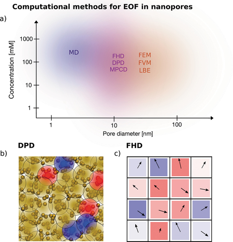
The downside is that atomistic simulations are limited in the spatial and temporal scales that can be resolved. Even with the ever-increasing availability of computational resources, an intermediate scale exists (i.e. mesoscale) that requires more details than continuum methods to be described and yet is out of reach of atomistic approaches. Any technique suitable to tackle such problems falls in the quite broad category of mesoscale methods. Mesoscale methods represent a heterogeneous set of techniques, that sometimes have little in common among one another. For a given problem, a specific method is usually better suited than another, depending on factors such as the geometry of the system, the boundary conditions and the presence of moving nanoparticles or biomolecules. In the following paragraph, we focus on mesoscale techniques that can be used to simulate nanoconfined electrolyte solutions and electroosmotic flows, summarized in Figure 5a.

The diversity of mesoscale approaches calls for additional sub-classifications. One common discriminating feature is the model used to describe the fluid. This can be done as an extension of continuum methods, describing the fluid in terms of a velocity field, where properties such as viscosity and dielectric constant can be directly assigned. To account for finite-size effects, modifications to the dynamical equations or to the local properties can be added. We refer to these approaches as top-down models. Another possibility is to extend on molecular dynamics, and model the fluid by a set of mobile, coarse-grained particles that represent molecules or groups of molecules rather than single atoms. Interactions between fluid particles result in effective fluid properties, that are naturally modified by the confinement. We refer to these approaches as bottom-up. In the following, we focus on representative methods belonging to either category (Dissipative Particle Dynamics (DPD) for bottom-up and Fluctuating Hydrodynamics (FHD) for top-down) and provide a brief overview of some of other approaches. More insight, especially on these other mesoscale approaches, may be found for example in [201].

Figure 5. Methods to simulate EOF. a) Diagram of the different computational methods available to simulate EOF in nanopores, classified according to the pore size and concentration of the simulated system. The colored area surrounding the name of the method shows the range of systems which are most suited to be simulated. The areas are shaded since the choice has to take into account additional system-specific factors, e.g. presence of moving particles, importance of thermal fluctuations, importance of ion-specific effects. The blue area represents an atomistic method, all-atom MD. The violet area represents a group of mesoscale methods which do not have atomistic resolution but still are able to model the thermal fluctuations of the system, namely Fluctuating Hydrodynamics, Dissipative Particle Dynamics and Multi-Particle Collision Dynamics. The Orange area refers to different computational methods to solve PNP-NS equations, such as Finite Volume Method, Finite Element Method and to Lattice Boltzmann Electrokinetics. b) Sketch of the simulation set up of a bottom-up approach (DPD). Each DPD particle is represented by a big blob delimited by a black circle, which can be yellow (neutral solvent), blue (positively charged) or red (negatively charged). The blobs overlap as a consequence of the weak repulsive interactions typical of DPD simulations. In the background, a possible atomistic system represented by the DPD particles, with solvent atoms (yellow), positive ions (blue) and negative ions (red). c) Sketch of the simulation set up of a top-down approach (FHD). The fluid is divided into cells, each of which has a fluctuating velocity, here represented as an arrow, and a charge arising from the ion density fluctuations, here represented as a colored box, for positive (blue) and negative (red) charges.

4.1. Bottom-up approaches

Bottom-up approaches model the fluid as a set of interacting particles, whose position and velocities are updated according to rules, which preserve total momentum, see Figure 5b. The hydrodynamic behavior of the fluid hence arises from the microscopic interactions between the mesoscale particles.

Dissipative particle dynamics

The DPD model was introduced by Hoogerbrugge and Koleman in 1992 [202] as a stochastic differential equations model. Its statistical mechanics properties were studied a few years later by Español and Warren [203], who obtained a fluctuation–dissipation relation between the deterministic and stochastic parts of the equations. The original DPD set of equations determining the motion of all the particles representing the fluid reads

(10) $\frac{d{\mathit{x}}_i}{dt}={\mathit{v}}_i,$(10)

(11) $m\frac{d{\mathit{v}}_i}{dt}=\sum _{j\ne i}{\mathit{F}}_{ij}^C+{\mathit{F}}_{ij}^D+{\mathit{F}}_{ij}^S,$(11)

where ${\mathit{x}}_i$ is the position of the $i^{\mathrm{t}\mathrm{h}}$ particle, ${\mathbf{v}}_i$ its velocity, $m$ its mass and ${\mathit{F}}_{ij}^C$, ${\mathit{F}}_{ij}^D$, ${\mathit{F}}_{ij}^S$ are three pairwise radial forces, respectively, a weakly repulsive conservative force, a dissipative force proportional to the radial component of the velocity difference between particles, and a stochastic force proportional to a white noise process [204]. The magnitude of the three forces is determined by parameters which define the properties of the fluid, and decreases with the distance between the particles, vanishing if the interparticle distance is larger than a cutoff radius.

The formulation of DPD has been modified in several ways to represent increasingly more complex fluids and systems. First, in the original model, the conservative force decreases linearly with the interparticle distance, limiting the range of equations of state of the modeled fluid. Modifications to the conservative force introducing a local density variable allow fluids with different equations of state to be simulated [205–207]. Second, the addition of an internal energy variable for each particle and a stochastic equation governing energy exchange between particles enables simulations with temperature gradients and heat flows [208–210]. Finally, interactions with fixed DPD particles representing the solid surface enable simulations of nanoscale flows, including hydrodynamic interactions between colloids and the effect of confining walls with different slip lengths [211–216].

Two different strategies can be adopted to represent an electrolyte solution and study charged systems with DPD. One possibility is to use charged DPD particles, directly representing the ions. Dynamics are given by the original DPD equations, with the addition of Coulombic forces in Eq. (11)(11) $m\frac{d{\mathit{v}}_i}{dt}=\sum _{j\ne i}{\mathit{F}}_{ij}^C+{\mathit{F}}_{ij}^D+{\mathit{F}}_{ij}^S,$(11) . Simulations of electrolyte solutions including polyelectrolytes have been conducted [217], even in an electroosmotic planar channel setting [218]. Smoothed charges are used to avoid artificial ion pairing due to the weak repulsive interactions ${\mathit{F}}_{ij}^C$ compared to the Coulombic attraction [219]. Polarizability effects can also be included, employing coarse-grained DPD water molecules or proteins [220,221].

Another possibility to model electrolyte solutions is to consider the DPD particle as a portion of solution rather than as a group of solvent molecules or a single ion. This requires to represent the quantity of ions carried by the DPD particle as an independent variable with additional evolution equations [222,223], an approach that has proven useful for the modeling of solutions in advection-diffusion-reaction problems [224] and can also provide control on the fluid equation of state including ion-specific effects such as excluded volume [223]. Using a separate evolution equation for the ion dynamics has an advantage in terms of scalability of the system size since multiple ions can be represented by a single DPD particle. Ion transport models are also more versatile as they are governed by an independent set of equations and parameters.

While noteworthy progress has been made in recent years to simulate electrolyte solutions in confined environments with DPD, some issues remain to be tackled. Most importantly, tuning transport coefficients, the fluid’s equation of state, slippage and polarizability is crucial to accurately model the fluid’s properties. Yet, it is not straightforward due to the bottom-up nature of DPD: forces either have to be derived from atomistic models via a coarse-graining procedure [225] or calibrated to map fluid properties [216,223,226,227]. Reproducing the properties of existing fluids is critical to widen the set of fluids accessible with DPD. This requires additional efforts to improve both DPD models of electrolyte solutions and the calibration of the fluid properties.

Multi-particle collision dynamics

Another possible bottom-up approach is Multi-Particle Collision Dynamics (MPCD) [228]. Here, the fluid is represented as a set of particles with position and velocity free to move continuously in space. Particle velocities are updated via a streaming step in which the positions are updated and a collision step in which the fluid domain is divided into cells of constant size, and the velocities of all the particles in each cell are rotated by a random vector that is different for each cell but identical for all particles in the same cell. Solute particles may be embedded into the MPCD description by treating them as fluid particles interacting with each other, propagating their positions according to standard MD algorithms instead of having a simple streaming step [229]. In this way, effects due to the finite size of ions can be taken into account. MPCD has been used to study nanoscale systems such as polymer translocation dynamics through nanopores [230] and EOFs in planar channels [229].

Lattice-Boltzmann

In the Lattice-Boltzmann (LB) approach the fluid is modeled as a set of particles with position and velocity. One key difference here with respect to other approaches is that the particles evolve on a lattice and represent the probability density function (or density) of the fluid [231]. Similarly to MPCD, the dynamics that determine the fluid behavior include (i) a collision step in which particle velocities are updated according to a collision operator that preserves total momentum, and (ii) a streaming step in which the distribution of particles evolves according to their velocities. The LB method has been applied to simulate electrolyte solutions at the nanoscale [201,232] and electrokinetic phenomena, combining LB for hydrodynamics and the resolution of convection-diffusion equations for charges, an approach known as Lattice Boltzmann Electrokinetics (LBE) [233–235].

4.2. Top-down approaches

Shifting perspectives, top-down approaches describe fluid flow in a continuous fashion, see Figure 5c, with enhanced fundamental equations to include details that are relevant at the nanoscale. An important tool to account for fluctuations at the nanoscale is called Fluctuating Hydrodynamics (FHD). We review how to use this tool in the context of electroosmosis below, and give some brief insight into other top-down approaches.

Fluctuating ionic concentration field in fluctuating hydrodynamic field

The first step is to introduce fluctuations in the hydrodynamic equations for conservation of momentum and mass balance Eq. (5)(5) $\rho \frac{\mathrm{\partial }\mathit{u}}{\mathrm{\partial }t}+\rho \mathit{u}\cdot \text{bnabla}\mathit{u}\mathbf{=}\text{bnabla}\cdot \text{r}\mathbf{\Sigma }\mathbf{-}{\rho }_{\mathrm{e}}\text{bnabla}\mathbf{\Phi }\mathbf{,}$(5) and (6(6) $\text{bnabla}\cdot \mathit{u}=0,$(6) ), as in [236,237]

(12) $\rho \frac{\mathrm{\partial }\mathit{u}}{\mathrm{\partial }t}+\rho \mathit{u}\cdot \text{bnabla}\mathit{u}=\text{bnabla}\cdot \mathbf{\Sigma }+\text{bnabla}\cdot \mathbf{S}-{\rho }_e\text{bnabla}\mathrm{\Phi },$(12)

(13) $\text{bnabla}\cdot \mathit{u}=0$(13)

where $\mathbf{\Sigma }=-p\mathit{I}+2\eta \sigma$ is the stress tensor defined in Eq. (8(8) $\mathbf{\Sigma }=-p\mathit{I}+\mathit{2}\eta \sigma ,$(8) ), $\mathit{S}$ is a random stress tensor satisfying the fluctuation-dissipation theorem, whose components are white in space and time, with mean zero, and $⟨S_{ij}(\mathit{r},t)S_{kl}(\mathit{r}{ }^{\mathbf{\prime }},t{ }^{\mathrm{\prime }})⟩=2\eta k_{B}T({\delta }_{ij}{\delta }_{kl}+{\delta }_{il}{\delta }_{jk})\delta (\mathit{r}-\mathit{r}{ }^{\mathbf{\prime }})\delta (t-t{ }^{\mathrm{\prime }})$. Note that here the fluid density is assumed to be uniform and constant but extensions are possible [237]. The advantage of Eq. (12)(12) $\rho \frac{\mathrm{\partial }\mathit{u}}{\mathrm{\partial }t}+\rho \mathit{u}\cdot \text{bnabla}\mathit{u}=\text{bnabla}\cdot \mathbf{\Sigma }+\text{bnabla}\cdot \mathbf{S}-{\rho }_e\text{bnabla}\mathrm{\Phi },$(12) is to keep a continuous, high-level description of the fluid, that does not rely on resolving individual molecular collisions, or on maintaining a constant temperature heat bath. Yet, Eq. (12)(12) $\rho \frac{\mathrm{\partial }\mathit{u}}{\mathrm{\partial }t}+\rho \mathit{u}\cdot \text{bnabla}\mathit{u}=\text{bnabla}\cdot \mathbf{\Sigma }+\text{bnabla}\cdot \mathbf{S}-{\rho }_e\text{bnabla}\mathrm{\Phi },$(12) does describe thermal fluctuations at small scales, conserves momentum, and is consistent with fluctuation-dissipation. Note that we keep the non-linear term in the Navier-Stokes equation for now; as in non-equilibrium cases typical of electroosmosis, equations have to be linearized around non-zero average velocity fields.

Numerous studies show an important impact of fluctuations in confinement as modeled through Eq. (12)(12) $\rho \frac{\mathrm{\partial }\mathit{u}}{\mathrm{\partial }t}+\rho \mathit{u}\cdot \text{bnabla}\mathit{u}=\text{bnabla}\cdot \mathbf{\Sigma }+\text{bnabla}\cdot \mathbf{S}-{\rho }_e\text{bnabla}\mathrm{\Phi },$(12) . The equations may be solved analytically in specific cases to investigate the overall transport quantities. For example, for confined fluids, fluctuations impact the de-wetting transition [238] and bubble formation by cavitation [239]. Memory effects in the center of mass diffusion have also been identified [240]. Finally, fluctuations of the surrounding confining material can enhance ensemble diffusion [67]. More generally, the equations are amenable to numerical solutions of the fluid velocity field on a grid. Such numerical solutions require careful discretization of the noise operator [241], in particular to properly account for confining boundaries [242], and of the forces at play, especially when looking at fluid-structure interactions where the structure also has thermal fluctuations [243,244].

To describe ions in such fluctuating fields, at low enough densities, one can use continuous concentration fields. As for the fluid, we can update the continuity equation Eq. (4)(4) $\frac{\mathrm{\partial }{c}_{\alpha }}{\mathrm{\partial }t}+\text{bnabla}\cdot \left(c_{\alpha }\mathit{u}+j_{\alpha }\right)=0,$(4) for each species $\alpha$ with a stochastic term [236,245,246]

(14) $\frac{\mathrm{\partial }{c}_{\alpha }}{\mathrm{\partial }t}=-\text{bnabla}\cdot (c_{\alpha }\mathit{u}+{\mathit{j}}_{\alpha }+{\mathit{F}}_{\alpha }^S)$(14)

where we take ${\mathit{j}}_{\alpha }$ to be given by the constitutive ion flux Eq. (9)(9) ${\mathit{j}}_{\alpha }=-D_{\alpha }\left(\text{bnabla}{c}_{\alpha }+c_{\alpha }\frac{q{Z}_{\alpha }}{k_{B}T}\text{bnabla}\mathrm{\Phi }\right),$(9) and ${\mathit{F}}_{\alpha }^S$ a stochastic flux that satisfies fluctuation-dissipation,

(15) ${\mathit{F}}_{\alpha }^S=\sqrt{2D_{\alpha }{c}_{\alpha }}\mathcal{Z}$(15)

where $\mathcal{Z}$ is a Gaussian vector with uncorrelated components in space and time. The fluctuating correction can also be recovered through density functional theory [247].

Such a formulation is interesting as it allows one to efficiently investigate fluctuation-driven behavior, both numerically and analytically. This approach has been used to identify enhanced charge transport due to fluid fluctuations, that result in ion concentration corrections to diffusion, sometimes leading to negative diffusion [245] or enhanced electric conductivity [248]. In other contexts, giant fluctuations may appear at interfaces with concentration gradients, which can be enhanced by applied electric fields [237].

The effect of fluctuations on electroosmosis has not yet been assessed in detail, and numerous questions are open. Such problems are now accessible to simulations, as confining boundary conditions have already been successfully implemented [249] and EOFs have been simulated in FHD for ionic liquids [250]. One might expect fluctuation enhanced behavior of the EOF, as identified for the electrical conductivity [248], yet the mechanisms remain to be unraveled. Furthermore, FHD represents a good starting point to rationalize further the effect of fluctuations at the boundaries, for example originating from charge regulation on surfaces [120,251], which should be crucial for EOF. Overall, this is a completely open question where combined mathematical frameworks and numerical investigations have to be built.

Particle ionic field in fluctuating hydrodynamic field

At high ionic densities, or in strongly confined systems, continuum approaches are not physically or numerically relevant. In fact, since the Debye length scales as ${\lambda }_D\sim c^{-1/2}$, where $c$ is the ionic concentration, the number of ions in a grid cell is at most ${\lambda }_D^{3}c\sim c^{-1/2}$ (since the discretization grid length is at least smaller than ${\lambda }_D$). Hence, numerically, the number of ions per cell at high concentrations is too small for a continuum description of ions to be sensible. Notice, that, physically, at very high concentrations, ${\lambda }_D$ approaches the molecular scale ${\lambda }_D\stackrel{<}{\sim \phantom{{ }_x}}1\mathrm{n}\mathrm{m}$ and a continuum description with cell sizes smaller than ${\lambda }_D$ is also questionable at that scale. Therefore, at high concentrations, a natural top-down simulation improvement is to resort to a discrete description for the ions [252,253], but keep a continuous description for the solvent velocity field. To avoid common difficulties associated with tracking a particle of finite size in fluid flow most works rely on methods such as Immersed Boundaries (IB) [254–256] or fluctuating force coupling methods [257,258], which effectively smear the particle on the velocity grid. This forms a hybrid, top-down approach. While such mixed approaches remain quite novel, especially in their applications to charged species [252], they could capture effects that occur on the molecular scale due to fluctuating hydrodynamics, especially as they are well suited to bridge the scales between large reservoirs and confined pores.

Smoothed dissipative particle dynamics

Another top-down approach is a top-down version of DPD, known as Smoothed Dissipative Particle Dynamics (SDPD) [259]. It consists in a discretization of the Navier-Stokes equations into a particle system instead of a fixed mesh, in which each particle moves according to its velocity, while the continuous velocity field (and any other relevant field) can be interpolated using bell-shaped functions centered on each particle. The momentum balance equation can then be used to update the velocity of each particle. This approach can be considered as a Lagrangian discretization of the Navier-Stokes equations, which includes thermal fluctuations in a consistent way. The advantage with respect to DPD techniques is that properties such as viscosity are inputs of the model and don’t have to be calibrated. The introduction of charged species in the model would require either considering some charged fluid particles as ions (hence in a mixed bottom-up/top-down approach), similar to what is done in DPD with explicit ions [218], or the introduction of an ionic concentration variable (somehow similar to DPD approaches in [222,223]) with an additional set of equations based on the continuity equation Eq. (4)(4) $\frac{\mathrm{\partial }{c}_{\alpha }}{\mathrm{\partial }t}+\text{bnabla}\cdot \left(c_{\alpha }\mathit{u}+j_{\alpha }\right)=0,$(4) .

5. Technological applications of EOF

From a technological perspective, EOF is attractive as it provides the unique possibility to induce and control a flow by easily tuning the externally applied voltage drop. Compared to standard pressure-driven flux, this is experimentally extremely convenient at the micro to nanoscale as it avoids common issues such as membrane fracture [260]. EOF can be further manipulated by modifying the system design through the surface properties of the channel walls as discussed in section 1.2.

In the last decades, this has led to a large variety of applications of EOF at the microscale such as pumps [27], micromixers [261], and transdermal drug delivery systems [262]. Some of these applications have been recently extended down to the nanoscales, such as pumps [263–265]. Nanofluidic pumps can be used in direct current mode [263] exploiting intrinsic selectivity due for instance to fixed charge accumulation at the pore walls as in Figure 2a-c. They can also be used in alternate current mode, where, to achieve a net EOF flow after a voltage cycle, current rectification is provided by pore asymmetry [264], induced charge [38] or unequal ions mobilities [266,267]. The latter does not necessarily require an asymmetric porous membrane and, consequently, could simplify the fabrication process. This possibility extends the variety of technological solutions aimed at harnessing EOF and remains to be explored experimentally. Further interesting recent progress in EOF includes chemoresponsive pumps where the flow decreases when a given species reaches a threshold concentration [265] and pumps integrated in flexible materials such as fabric [268]. Moreover, other purely nanoscale applications have emerged such as the development of soft actuators [269] and the design of a nanorobot able to move along a solid-state surface [270].

In the following sections, we focus on one specific application of EOF at the nanoscale, namely the electrohydrodynamic manipulation of nanoparticles and molecules to control their interaction with a nanopore or a nanoporous membrane. This is particularly relevant in nanopore sensing devices, see Section 5.1, and it may also be important for applications to blue energy and desalination, see Section 5.2.

Figure 6. Nanopore/nanoparticle interactions: the role of EOF in applications. a) Nanopore sensing. The properties of a translocating particle are deduced from the signature it leaves in the electric current trace. Indeed, when the particle enters the pore, it partially blocks the ion flow and, consequently, the electric current is reduced (stage 2, violet). The capture of molecules and particles to be analyzed needs to be favored. This may be particularly challenging when particles are not charged. In this respect, EOF constitutes a promising approach since it may induce particle capture regardless of their charge. b) Blue energy and c) Filtration. The interaction between dispersed nanoparticles and nanoporous membrane may impact the performance of desalination, filtration and blue energy harvesting membranes since nanoparticles can clog the pores (fouling). EOF can be employed to generate a flow to clean the membrane (backwashing). d) Particle capture. The three phases of the capture in a nanopore sensing device. i) Bulk diffusion. Far from the pore, electrophoresis and electroosmosis are negligible. Hence, the dynamics are dominated by Brownian motion, until the particle reaches the pore capture region. ii) Funneling. Once the particle is in the capture region, Brownian motion competes with electric and hydrodynamic forces. If the latter are directed towards the pore, the particle experiences a funnel-like field: the closer the particle to the pore entrance, the larger the attractive force. iii) Pore docking. The particle finally reaches the pore entrance region, where molecular pore–particle interactions become relevant. e) Capture frequency of a positively charged particle, as a function of $\mathrm{\Delta }V$ from a theoretical model [11] showing the competition/cooperation between EOF and electrophoresis depending on the wall surface charge $q_w$. The black line refers to pure electrophoresis ($q_w=0$), red and blue lines to positively and negatively charged walls. Panel d-e adapted from [11]. Panel d-iii was realized using the VMD software [271].

5.1. EOF enhanced nanopore sensing

One of the most widely studied applications of EOF at nanoscale is nanopore sensing. Nanopore sensing is based on the presence of particles inside the pore [9,272]. The molecular properties of analytes are inferred by the alteration of the electric current flowing through the nanopore [8,33,273] (Figure 6a). This approach is usually referred to as resistive pulse and it is, by far, the most commonly employed strategy for nanopore sensing. Other approaches have been proposed, such as acquisition of the transverse tunneling current along the substrate plane [274], fluorescence signals elicited by a laser light [275] and FRET spectroscopy to sense the deformation of a biopore due to the molecule’s passage [276]. Also plasmonic nanostructures have been recently used in nanopore sensors enhancing optical spectroscopy, local temperature control and molecule thermophoresis [277,278].

A sketch of the resistive pulse approach is reported in Figure 6a. When the particle is outside the pore, the electric current fluctuates around a base level (stage 1, grey). When the particle enters the pore, it partially blocks the ion flow and, consequently, the electric current is reduced (stage 2, violet). When finally the particle leaves the pore, the current returns to its empty pore value (stage 3, grey). There are three main requirements that a nanopore sensing device needs to fulfill. First, molecules dispersed in the reservoirs must enter the nanopore (capture control). Then, the captured molecule must reside inside the pore for enough time to record a stable current signal (translocation/residence control) and, finally, signals coming from different molecules (or different parts of the same molecule, e.g. single monomers when the aim is polymers sequencing [8]) must be different from each other (distinguishability). EOF has been shown to be a useful method to control the capture, as it will be described in the following.

The capture of a molecule into a nanopore is a complex process governed by the interplay among Brownian diffusion, hydrodynamics, physico-chemical and electrostatic effects. In general, we can roughly split the capture processes in three main phases, see Figure 6d [11]. (i) Bulk diffusion: Far from the pore, the electroosmotic drag and electrophoresis are, in essence, negligible. Here, the particle dynamics are dominated by Brownian motion. (ii) Funneling: Brownian motion occasionally brings a particle so close to the pore that electric and hydrodynamic forces start to be relevant. Supposing that the resultant of these actions is directed toward the pore, the particle experiences a funnel-like field: the closer the particle is to the pore, the larger the attractive force. (iii) Pore docking: The particle finally reaches the pore entrance, where pore-particle molecular interactions become relevant and often dominant.

EOF acts on both funnelling and pore docking phases. For highly charged molecules, such as DNA, the main driver of the funneling phase is electrophoresis. However, when the analyte has a low net charge, the electrophoretic force becomes negligible. Proteins are a relevant class of biomolecules for which this is the case. Indeed, they are either positively or negatively charged and, in general, their charge depends on the solution pH so electrophoresis does not constitute a general systematic method for protein capture in nanopores. Therefore, an EOF directed toward the pore appears as a promising alternative to favor capture. Several works reported EOF induced capture for proteins and peptides [12,14,15,77,279,280]. In Asandei et al. [15], a positively charged peptide was captured in a biological pore ($\alpha$-HL), against electrophoresis. The EOF was tuned by altering the protonation state of residues in the pore lumen decreasing the pH of the solution to 2.8 (see Figure 4 for MD simulation data on the effect of pH in EOF through $\alpha$-HL). Similar evidence has been reported in [76] where a globular protein is captured by ClyA pore. A recent approach to exploit EOF for protein capture and trapping is to dock a DNA-origami sphere onto a solid-state nanopore. The sphere partially seals off the nanopore and, altering the distribution of ions in the pore region, gives rise to an EOF [77]. The employment of EOF to enhance the capture of the analyte is not limited to proteins. EOF has proven relevant for sensing relatively large analytes with low charge, such as viruses in solid-state pores [281], as well as antibiotics and sugars in biological pores [13,282,283].

In experimental studies on molecule capture in nanopores, the role of EOF (and electrophoresis) on funneling and pore docking phases can hardly be disentangled. For biological pores, for instance, any mutation on the pore entrance aimed at altering the interaction between pore and molecule may also change the EOF. In this respect, MD simulations may help to isolate the effect of EOF on the molecule’s entry, as shown for instance in [284] using free-energy calculations.

Analytic theoretical frameworks trying to model particle capture under the concurrent action of electric forces, EOF advection, and Brownian motion have been proposed with the aim of understanding the overall dependence of the capture frequency as a function of the magnitude of the applied voltage [11,73,285]. These analytical approaches, based in essence on the solution of the advection-diffusion equation, can also be used to analyze the cooperation/competition between electrophoresis and electroosmosis in different conditions, Figure 6e. Although these theoretical routes may provide useful guidelines for preliminary designs of systems enhancing the capture of the desired molecules, a precise determination of the role of EOF in nanopore sensing would largely benefit from the employment of the various computational approaches briefly discussed in the present review.

As a final remark, EOF may be employed also for translocation control. Tsutsui et al. [286] showed that it is possible to slowdown the particle’s translocation through a solid-state nanopore controlling the EOF via a voltage-gated mechanism. Zhang et al. [287] showed that for a solid state nanopore, the translocation of proteins slows down when the pore diameter is larger than the pore length. They attributed this effect to a reduction of the EOF in the center of the channel, an effect that is evident in continuum simulations, see e.g. Figure 3c.

5.2. Role of EOF in blue energy and desalination

Besides sensing, nanopores are key elements of emerging technologies with promising outcomes to solve global challenges. For example nanopore based-membranes can harvest blue energy, a sustainable energy [288] and can improve access to clean water through high-performance filtration and desalination [289].

In blue energy harvesting, where a salinity gradient is converted into electric power, a membrane selective for positive (or negative) ions separates two reservoirs containing solutions with different salinities, e.g. sea and fresh water [288,290]. Ions diffuse from the high salinity to the low salinity chamber. Assuming as in Figure 6b that the membrane is cation selective, the positive charge flux will be larger than the negative one, resulting in a net electric current. For desalination applications, instead, the membrane hinders the passage of all the ions [289,291,292]. In such devices, a pressure is applied on the high concentration chamber and fresh water is obtained on the other side of the membrane, see Figure 6c. A similar working principle is used to purify water from contaminants in ultrafiltration processes [293]. In both blue energy and water treatment systems, dispersed nanoparticles can clog the pore (membrane fouling [290,294]), dramatically reducing the performance of real-life systems with respect to laboratory set-ups. In this scenario, EOF may be used to induce a flow to clean the membrane from particles (backwashing [295,296]). The decrease of the membrane performance is also due to ion concentration polarization near the membrane that, again, can potentially be attenuated with EOF [297]. It is worth noting that in these two technologies the voltage $\mathrm{\Delta }V$ is not the only applied load to the systems and also concentration and pressure differences between the two reservoirs need to be considered, making the transport phenomenon more intricate [298].

One central and open question for all these technological applications is: Given an electrolyte solution containing a mixture of nanoparticles, how can we design the nanopore and tune the operating conditions to facilitate the capture of specific nanoparticles and/or hinder undesired ones? In answering this question, EOF plays a crucial role since it acts on all the dispersed molecules regardless of their charge and dipole, constituting a more generic way of manipulating particles in nanopore systems.

6. Future outlook

In this review, we discussed mechanisms to control EOF in nanopores, the main computational techniques used to predict EOF and some of its recent applications in sensing, energy and filtration. While such applications are very promising, the understanding of the experimentally observed phenomena often requires computer simulations to catch the large variety of physical effects influencing EOF in nanopores. Explaining experimental observations has been, up to now, the most common use of computer simulations of EOF when combined with experiments, see, e.g. [15,98,279,299]. Yet quantitative prediction is crucial to address the challenge of designing new generation nanofluidic devices exploiting EOF. From the computational point of view, this requires a careful selection of the model and the numerical technique and to take into account the relevant effects in the system for all parameters considered, while using a minimal amount of computational resources. Atomistic simulations are already well established and, thanks to the spread of GPU computing, they will probably be more and more used in the future. Indeed, even lab scale GPU workstations are now able to perform simulations involving hundreds of thousands of atoms. This is usually sufficient to obtain a reliable prediction of EOF in relatively small pores such as $\alpha$-HL or FraC. Supercomputers are still needed for larger systems and, in particular, for simulation campaigns aimed at exploring different parameters, such as the effect of pore modifications or of electrolyte composition on EOF. Nowadays, typically these simulation campaigns require weeks or months and are mainly devoted to fundamental research projects. They are not yet easily scalable to industrial developments where fast quantitative prediction are needed to optimize device performance. Hence, a real breakthrough in nanopore technology will only be achieved via computational approaches that enable to efficiently explore a huge variety of nanopore systems and operational conditions on standard workstations within a computational time of a few days. Such tools will pave the way for modern design practices at the nanoscale, harvesting modeling and optimization techniques currently only used at larger scales. In this respect, continuum and mesoscale modeling appear as the natural choice for fast simulation strategies. Although no technique is nowadays able to robustly guarantee an a priori quantitatively accurate prediction for EOF in real nanopores, some of the recent progress in including nanoscale effects in continuum and mesoscale approaches discussed in this review are quite promising. We expect that they will contribute to the development of a new generation of computational tools for nanopore design.

Acknowledgments

The authors are grateful for fruitful discussions with Aleksandar Donev, Brennan Sprinkle and Francesco Viola. The authors would also like to thank the researchers that provided us high quality figures, S.L. Zhang Y. Yao for Figure 2h, G. Maglia and K. Willems for (Figure 3(a,d)), M. Gracheva for (Figure 3(b-c)), A. Aksimentiev for (Figure 4(c-f)). S.M. acknowledges funding from the MolecularControl project, European Union’s Horizon 2020 research and innovation programme under the Marie Skłodowska-Curie grant award number 839225. S.M. was supported in part by the MRSEC Program of the National Science Foundation under Award Number DMR-1420073. PM acknowledge funding by the Deutsche Forschungsgemeinschaft (DFG, German Research Foundation) Project-ID 416229255 SFB 1411. GDM and MC acknowledge the computational resources provided by the CSCS Swiss National Supercomputing Centre (Project-ID s1026) and Italian CINECA (Projects IsB21_FLOWYAX and IsC86_CSGGEOF). MB was supported by Università Italo-Francese under Vinci grant (project C3-1352).

Disclosure statement

No potential conflict of interest was reported by the author(s).

Additional information

Funding

This research is part of a project that has received funding from the European Research Council (ERC) under the European Union’s Horizon 2020 research and innovation programme (grant agreement No. 803213); Deutsche Forschungsgemeinschaft [416229255 SFB 1411]; MRSEC National Science Foundation [DMR-1420073]; Marie Sklodowska-Curie Actions [839225].

Notes

1. In the literature on charge accumulation at liquid-solid interfaces, different terms are used to describe specific phenomena occurring in this thin interfacial layer. Examples are the Stern layer, the Gouy-Chapman diffuse layer and the electric double layer. In this review, we do not need to enter in the specific definitions of these layers and, in line with part of the recent literature and textbooks [18], we refer to the region in which the ions accumulate/deplete as the Debye layer.

2. Voltage gated nanopores described in this review should not be confused with voltage gated ion channels [52]. The main difference is that in voltage gated ion channels the transmembrane voltage induces conformational changes which influence their transport properties. In the voltage gated nanopores described here, an additional external voltage is applied to the membrane, providing independent control of transmembrane voltage and surface potential at the membrane.

3. Except around a non-zero, large, average flow, where the left hand side has to be linearized.

4. Such that the translocation time of an ion is much longer than the typical insertion time.

References

- Reuss FF. Notice sur un nouvel effect de 1ʹélectricité galvanique. Mem Soc Imp Nat Moscou. 1809;2:3227.
- Porrett R Jr. Curious galvanic experiments. Ann Philos. 1816;8:74–53.
- Biscombe CJC. The discovery of electrokinetic phenomena: setting the record straight. Angew Chem. 2017;56:8338–8340.
- Kirby BJ. Micro-and nanoscale fluid mechanics: transport in microfluidic devices. Cambridge University Press; 2010.
- Haywood DG, Saha-Shah A, Baker LA, et al. Fundamental studies of nanofluidics: nanopores, nanochannels, and nanopipets. Anal Chem. 2015;87:172–187.
- Yusko EC, Ran A, Mayer M. Electroosmotic flow can generate ion current rectification in nano-and micropores. ACS Nano. 2010;4:477–487.
- Balme S, Picaud F, Manghi M, et al. Ionic transport through sub-10 nm diameter hydrophobic high-aspect ratio nanopores: experiment, theory and simulation. Sci Rep. 2015;5:1–14.
- Chinappi M, Cecconi F. Protein sequencing via nanopore based devices: a nanofluidics perspective. J Phys. 2018;30:204002.
- Bayley H, Braha O, Gu L-Q. Stochastic sensing with protein pores. Adv Mater. 2000;12:139–142.
- Xue L, Yamazaki H, Ren R, et al. Solid-state nanopore sensors. Nat Rev Mater. 2020;5:931–951.
- Chinappi M, Yamaji M, Kawano R, et al. Analytical model for particle capture in nanopores elucidates competition among electrophoresis, electroosmosis, and dielectrophoresis. ACS Nano. 2020;14:15816–15828.
- Saharia, J., Bandara, Y. N. D., Karawdeniya, B. I., Hammond, C., Alexandrakis, G., & Kim, M. J. 2021. Modulation of electrophoresis, electroosmosis and diffusion for electrical transport of proteins through a solid-state nanopore. RSC advances, 11(39), 24398–24409.
- Boukhet M, Piguet F, Ouldali H, et al. Probing driving forces in aerolysin and α-hemolysin biological nanopores: electrophoresis versus electroosmosis. Nanoscale. 2016;8:18352–18359.
- Huang G, Willems K, Soskine M, et al. Electro-osmotic capture and ionic discrimination of peptide and protein biomarkers with frac nanopores. Nat Commun. 2017;8:1–11.
- Asandei A, Schiopu I, Chinappi M, et al. Electroosmotic trap against the electrophoretic force near a protein nanopore reveals peptide dynamics during capture and translocation. ACS Appl Mater Interfaces. 2016;8:13166–13179.
- Ermann N, Hanikel N, Wang V, et al. Promoting single-file dna translocations through nanopores using electro-osmotic flow. J Chem Phys. 2018;149:163311.
- Hsu W-L, Daiguji H. Manipulation of protein translocation through nanopores by flow field control and application to nanopore sensors. Anal Chem. 2016;88:9251–9258.
- Bruus H. Theoretical microfluidics. Vol. 18. Oxford university press Oxford; 2008
- Gouy M. Sur la constitution de la charge électrique à la surface d’un électrolyte. J Phys Theor Appl. 1910;9:457–468.
- Leonard Chapman D. Li. a contribution to the theory of electrocapillarity. London, Edinburgh, Dublin Philos Mag J Sci. 1913;25:475–481.
- Fogolari F, Brigo A, Molinari H. The poisson–boltzmann equation for biomolecular electrostatics: a tool for structural biology. J Mol Recog. 2002;15:377–392.
- Debye P, Hückel E. De la theorie des electrolytes. i. abaissement du point de congelation et phenomenes associes. Physikalische Zeitschrift. 1923;24:185–206.
- Smeets RMM, Keyser UF, Krapf D, et al. Salt dependence of ion transport and dna translocation through solid-state nanopores. Nano Lett. 2006;6:89–95.
- Tianji M, Balanzat E, Janot J-M, et al. Nanopore functionalized by highly charged hydrogels for osmotic energy harvesting. ACS Appl Mater Interfaces. 2019;11:12578–12585.
- Willems K, Ruić D, Lucas FLR, et al. Accurate modeling of a biological nanopore with an extended continuum framework. Nanoscale. 2020;12:16775–16795.
- Bétermier F, Cressiot B, Di Muccio G, et al. Single-sulfur atom discrimination of polysulfides with a protein nanopore for improved batteries. Communicat Mater. 2020;1:1–11.
- Wang X, Cheng C, Wang S, et al. Electroosmotic pumps and their applications in microfluidic systems. Microfluid Nanofluid. 2009;6:145–162.
- Green Y. Conditions for electroneutrality breakdown in nanopores. J Chem Phys. 2021;155:184701.
- Noh Y, Aluru NR. Ion transport in electrically imperfect nanopores. ACS Nano. 2020;14:10518–10526.
- Dong Z, Kennedy E, Hokmabadi M, et al. Discriminating residue substitutions in a single protein molecule using a sub-nanopore. ACS Nano. 2017;11:5440–5452.
- Ying C, Houghtaling J, Eggenberger OM, et al. Formation of single nanopores with diameters of 20–50 nm in silicon nitride membranes using laser-assisted controlled breakdown. ACS nano. 2018;12:11458–11470.
- Won Shin J, Yong Lee J, Do Hyun O, et al. Shrinkage and expansion mechanisms of sio 2 elliptical membrane nanopores. Appl Phys Lett. 2008;93:221903.
- Cressiot B, Oukhaled A, Patriarche G, et al. Protein transport through a narrow solid-state nanopore at high voltage: experiments and theory. ACS nano. 2012;6:6236–6243.
- Yameen B, Ali M, Neumann R, et al. Single conical nanopores displaying ph-tunable rectifying characteristics. manipulating ionic transport with zwitterionic polymer brushes. J Am Chem Soc. 2009;131:2070–2071.
- Bai J, Wang D, Nam S-W, et al. Fabrication of sub-20 nm nanopore arrays in membranes with embedded metal electrodes at wafer scales. Nanoscale. 2014;6:8900–8906.
- Cantley L, Swett JL, Lloyd D, et al. Voltage gated inter-cation selective ion channels from graphene nanopores. Nanoscale. 2019;11:9856–9861.
- Yao Y, Wen C, Pham NH, et al. On induced surface charge in solid-state nanopores. Langmuir. 2020;36:8874–8882.
- Di Muccio G, Morozzo Della Rocca B, Chinappi M. Geometrically induced selectivity and unidirectional electroosmosis in uncharged nanopores. arXiv preprint arXiv:2104 03390. 2021. https://doi.org/10.1021/acsnano.1c03017
- Letizia Bonome E, Cecconi F, Chinappi M. Electroosmotic flow through an α-hemolysin nanopore. Microfluid Nanofluid. 2017;21:96.
- Gu L-Q, Cheley S, Bayley H. Prolonged residence time of a noncovalent molecular adapter, β-cyclodextrin, within the lumen of mutant α-hemolysin pores. J Gen Physiol. 2001;118:481–494.
- Cao B, Zhao Y, Kou Y, et al. Structure of the nonameric bacterial amyloid secretion channel. Proc Nat Acad Sci. 2014;111:E5439–E5444.
- Wanunu M, Meller A. Chemically modified solid-state nanopores. Nano Lett. 2007;7:1580–1585.
- Lin K, Zhongwu L, Tao Y, et al. Surface charge density inside a silicon nitride nanopore. Langmuir. 2021.
- Chen P, Mitsui T, Farmer DB, et al. Atomic layer deposition to fine-tune the surface properties and diameters of fabricated nanopores. Nano Lett. 2004;4:1333–1337.
- Hoogerheide DP, Garaj S, Golovchenko JA. Probing surface charge fluctuations with solid-state nanopores. Phys Rev Lett. 2009;102:256804.
- Eggenberger OM, Ying C, Mayer M. Surface coatings for solid-state nanopores. Nanoscale. 2019;11:19636–19657.
- Lepoitevin M, Tianji M, Bechelany M, et al. Functionalization of single solid state nanopores to mimic biological ion channels: a review. Adv Colloid Interface Sci. 2017;250:195–213.
- Anderson BN, Muthukumar M, Meller A. ph tuning of dna translocation time through organically functionalized nanopores. ACS nano. 2013;7:1408–1414.
- Karmi A, Priya Sakala G, Rotem D, et al. Durable, stable, and functional nanopores decorated by self-assembled dipeptides. ACS Appl Mater Interfaces. 2020;12:14563–14568.
- Mayumi Fujinami Tanimoto I, Cressiot B, Jarroux N, et al. Selective target protein detection using a decorated nanopore into a microfluidic device. Biosens Bioelectron. 2021;183:113195.
- Kim D, Darve E. High-ionic-strength electroosmotic flows in uncharged hydrophobic nanochannels. J Colloid Interface Sci. 2009;330:194–200.
- Armstrong CM, Hille B. Voltage-gated ion channels and electrical excitability. Neuron. 1998;20:371–380.
- Guan W, Sylvia Xin L, Reed MA. Voltage gated ion and molecule transport in engineered nanochannels: theory, fabrication and applications. Nanotechnology. 2014;25:122001.
- Ren R, Zhang Y, Paulose Nadappuram B, et al. Nanopore extended field-effect transistor for selective single-molecule biosensing. Nat Commun. 2017;8:1–9.
- Sedra AS, Smith KC. Microelectronic circuits. In: Oxf ser elec series. Oxford University Press; 2010.
- Kalman EB, Sudre O, Vlassiouk I, et al. Control of ionic transport through gated single conical nanopores. Anal Bioanal Chem. 2009;394:413–419.
- Van Toan N, Inomata N, Toda M, et al. Ion transport by gating voltage to nanopores produced via metal-assisted chemical etching method. Nanotechnology. 2018;29:195301.
- Nam S-W, Rooks MJ, Kim K-B, et al. Ionic field effect transistors with sub-10 nm multiple nanopores. Nano Lett. 2009;9:2044–2048.
- Pérez-Mitta G, Marmisollé WA, Trautmann C, et al. An all-plastic field-effect nanofluidic diode gated by a conducting polymer layer. Adv Mater. 2017;29:1700972.
- Cheng C, Jiang G, Philip Simon G, et al. Low-voltage electrostatic modulation of ion diffusion through layered graphene-based nanoporous membranes. Nat Nanotechnol. 2018;13:685–690.
- Wang Y, Zhang H, Kang Y, et al. Voltage-gated ion transport in two-dimensional sub-1 nm nanofluidic channels. ACS Nano. 2019;13:11793–11799.
- Squires TM. Induced-charge electrokinetics: fundamental challenges and opportunities. Lab Chip. 2009;9:2477–2483.
- Läuger P, Lesslauer W, Marti E, et al. Electrical properties of bimolecular phospholipid membranes. Biochimi Biophys Acta (BBA) Biomembr. 1967;135:20–32.
- Bazant MZ, Squires TM. Induced-charge electrokinetic phenomena. Curr Opin Colloid Interface Sci. 2010;15:203–213.
- Wanunu M, Morrison W, Rabin Y, et al. Electrostatic focusing of unlabelled dna into nanoscale pores using a salt gradient. Nat Nanotechnol. 2010;5:160–165.
- Chinappi M, Luchian T, Cecconi F. Nanopore tweezers: voltage-controlled trapping and releasing of analytes. Phys Rev E. 2015;92:032714.
- Marbach S, Dean DS, Bocquet L. Transport and dispersion across wiggling nanopores. Nat Phys. 2018;14:1108–1113.
- Ming M, Grey F, Shen L, et al. Water transport inside carbon nanotubes mediated by phonon-induced oscillating friction. Nat Nanotechnol. 2015;10:692–695.
- Gravelle S, Netz RR, Bocquet L. Adsorption kinetics in open nanopores as a source of low-frequency noise. Nano Lett. 2019;19:7265–7272.
- Thorneywork AL, Gladrow J, Qing Y, et al. Direct detection of molecular intermediates from first-passage times. Sci Adv. 2020;6:eaaz4642.
- Marbach S. Intrinsic fractional noise in nanopores: the effect of reservoirs. J Chem Phys. 2021;154:171101.
- Tai Andrew Wong C, Muthukumar M. Polymer capture by electro-osmotic flow of oppositely charged nanopores. J Chem Phys. 2007;126:164903.
- Grosberg AY, Rabin Y. Dna capture into a nanopore: interplay of diffusion and electrohydrodynamics. J Chem Phys. 2010;133:10B617.
- Aksimentiev A, Schulten K. Imaging α-hemolysin with molecular dynamics: ionic conductance, osmotic permeability, and the electrostatic potential map. Biophys J. 2005;88:3745–3761.
- Bhattacharya S, Muzard J, Payet L, et al. Rectification of the current in α-hemolysin pore depends on the cation type: the alkali series probed by molecular dynamics simulations and experiments. J Phys Chem C. 2011;115:4255–4264.
- Soskine M, Biesemans A, Moeyaert B, et al. An engineered clya nanopore detects folded target proteins by selective external association and pore entry. Nano Lett. 2012;12:4895–4900.
- Schmid S, Stömmer P, Dietz H, et al. Nanopore electro-osmotic trap for the label-free study of single proteins and their conformations. bioRxiv. 2021.
- Mukherjee S, Goswami P, Dhar J, et al. Ion-size dependent electroosmosis of viscoelastic fluids in microfluidic channels with interfacial slip. Phys Fluids. 2017;29:072002.
- Kim S, Karrila SJ. Microhydrodynamics: principles and selected applications. Courier Corporation; 2013.
- Prohl A, Schmuck M. Convergent finite element discretizations of the navier-stokes-nernst-Planck-poisson system. ESAIM Math Modell Numer Anal. 2010;44:531–571.
- Sherwood JD, Mao M, Ghosal S. Electrically generated eddies at an eightfold stagnation point within a nanopore. Phys Fluids. 2014;26:112004.
- Cho C-C, Chen C-L, et al. Characteristics of combined electroosmotic flow and pressure-driven flow in microchannels with complex-wavy surfaces. Int J Ther Sci. 2012;61:94–105.
- Lauga E, Brenner M, Stone H. Microfluidics: the no-slip boundary condition. In: Springer handbooks. Springer; 2007. p. 1219–1240.
- Collis JF, Olcum S, Chakraborty D, et al. Measurement of navier slip on individual nanoparticles in liquid. Nano Lett. 2021.
- Bazant MZ, Vinogradova OI. Tensorial hydrodynamic slip. J Fluid Mech. 2008;613:125–134.
- Sendner C, Horinek D, Bocquet L, et al. Interfacial water at hydrophobic and hydrophilic surfaces: slip, viscosity, and diffusion. Langmuir. 2009;25:10768–10781.
- Huang DM, Sendner C, Horinek D, et al. Water slippage versus contact angle: a quasiuniversal relationship. Phys Rev Lett. 2008;101:226101.
- Chinappi M, Casciola CM. Intrinsic slip on hydrophobic self-assembled monolayer coatings. Phys Fluids. 2010;22:042003.
- Bakli C, Chakraborty S. Slippery to sticky transition of hydrophobic nanochannels. Nano Lett. 2015;15:7497–7502.
- Joly L, Ybert C. Emmanuel T, et al. Liquid friction on charged surfaces: from hydrodynamic slippage to electrokinetics. J Chem Phys. 2006;125:204716.
- Melnikov DV, Hulings ZK, Gracheva ME. Electro-osmotic flow through nanopores in thin and ultrathin membranes. Phys Rev E. 2017;95:063105.
- Malgaretti P, Pagonabarraga I, Miguel Rubi J. Entropic electrokinetics: recirculation, particle separation, and negative mobility. Phys Rev Lett. 2014;113:128301.
- Chinappi M, Malgaretti P. Charge polarization, local electroneutrality breakdown and eddy formation due to electroosmosis in varying-section channels. Soft Matter. 2018;14:9083–9087.
- Malgaretti P, Janssen M, Pagonabarraga I, et al. Driving an electrolyte through a corrugated nanopore. J Chem Phys. 2019;151:084902.
- Benzhuo L, Zhou YC. Poisson-nernst-Planck equations for simulating biomolecular diffusion-reaction processes ii: size effects on ionic distributions and diffusion-reaction rates. Biophys J. 2011;100:2475–2485.
- Davidson SM, Andersen MB, Mani A. Chaotic induced-charge electro-osmosis. Phys Rev Lett. 2014;112:128302.
- Laohakunakorn N, Keyser UF. Electroosmotic flow rectification in conical nanopores. Nanotechnology. 2015;26:275202.
- Laohakunakorn N, Thacker VV, Muthukumar M, et al. Electroosmotic flow reversal outside glass nanopores. Nano Lett. 2015;15:695–702.
- Ai Y, Zhang M, Joo SW, et al. Effects of electroosmotic flow on ionic current rectification in conical nanopores. J Phys Chem C. 2010;114:3883–3890.
- Manghi M, Palmeri J, Henn F, et al. Ionic conductance of carbon nanotubes: confronting literature data with nanofluidic theory. J Phys Chem C. 2021;125:22943–22950.
- Sherwood JD, Mao M, Ghosal S. Electroosmosis in a finite cylindrical pore: simple models of end effects. Langmuir. 2014;30:9261–9272.
- Dreyer W, Guhlke C, Müller R. Overcoming the shortcomings of the nernst–Planck model. Phys Chem Chem Phys. 2013;15:7075–7086.
- Marbach S, Yoshida H, Bocquet L. Osmotic and diffusio-osmotic flow generation at high solute concentration. i. mechanical approaches. J Chem Phys. 2017;146:194701.
- Ruurds De Groot S, Mazur P. Non-equilibrium thermodynamics. Courier Corporation; 2013.
- Fuhrmann J. Comparison and numerical treatment of generalised nernst–Planck models. Comput Phys Commun. 2015;196:166–178.
- Bandopadhyay A, Chakraborty S. Ionic size dependent electroosmosis in ion-selective microchannels and nanochannels. Electrophoresis. 2013;34:2193–2198.
- Hameed Chaudhry J, Comer J, Aksimentiev A, et al. A stabilized finite element method for modified poisson-nernst-Planck equations to determine ion flow through a nanopore. Commun Computat Phys. 2014;15:93–125.
- Qiao Y, Bin T, Benzhuo L. Ionic size effects to molecular solvation energy and to ion current across a channel resulted from the nonuniform size-modified pnp equations. J Chem Phys. 2014;140:174102.
- Siddiqua F, Wang Z, Zhou S. A modified poisson–nernst–Planck model with excluded volume effect: theory and numerical implementation. arXiv preprint arXiv:1801 00751, 2017.
- Sabri Kilic M, Bazant MZ, Ajdari A. Steric effects in the dynamics of electrolytes at large applied voltages. i. double-layer charging. Phys Rev E. 2007;75:021502.
- Sabri Kilic M, Bazant MZ, Ajdari A. Steric effects in the dynamics of electrolytes at large applied voltages. ii. modified poisson-nernst-Planck equations. Phys Rev E. 2007;75:021503.
- Fuhrmann J, Clemens Guhlke AL, Merdon C, et al. Induced charge electroosmotic flow with finite ion size and solvation effects. Electrochim Acta. 2019;317:778–785.
- Mouterde T, Ashok Keerthi ARP, Dar SA, et al. Molecular streaming and its voltage control in ångström-scale channels. Nature. 2019;567:87–90.
- Schlaich A, Knapp EW, Netz RR. Water dielectric effects in planar confinement. Phys Rev Lett. 2016;117:048001.
- Fumagalli L, Esfandiar A, Fabregas R, et al. Anomalously low dielectric constant of confined water. Science. 2018;360:1339–1342.
- Kavokine N, Marbach S, Siria A, et al. Ionic Coulomb blockade as a fractional wien effect. Nat Nanotechnol. 2019;14:573–578.
- Sokoloff JB. Enhancement of the water flow velocity through carbon nanotubes resulting from the radius dependence of the friction due to electron excitations. Phys Rev E. 2018;97:033107.
- Kavokine N, Robert A. Marie-Laure B, et al. Fluctuation-induced quantum friction in nanoscale water flows. arXiv preprint arXiv:2105 03413. 2021.
- Siwy Z, Fuliński A. Origin of 1/f α noise in membrane channel currents. Phys Rev Lett. 2002;89:158101.
- Secchi E, Niguès A, Jubin L, et al. Scaling behavior for ionic transport and its fluctuations in individual carbon nanotubes. Phys Rev Lett. 2016;116:154501.
- Knowles SF, Weckman NE, Lim VJY, et al. Current fluctuations in nanopores reveal the polymer-wall adsorption potential. Phys Rev Lett. 2021;127:137801.
- Kavokine N, Netz RR, Bocquet L. Fluids at the nanoscale: from continuum to subcontinuum transport. Annu Rev Fluid Mech. 2021;53:377–410.
- Murad S, Oder K, Lin J. Molecular simulation of osmosis, reverse osmosis, and electro-osmosis in aqueous and methanolic electrolyte solutions. Mol Phys. 1998;95:401–408.
- Zhou W, Qiu H, Guo Y, et al. Molecular insights into distinct detection properties of α-hemolysin, mspa, csgg, and aerolysin nanopore sensors. J Phys Chem A. 2020;124:1611–1618.
- Aksimentiev A, Heng JB, Timp G, et al. Microscopic kinetics of dna translocation through synthetic nanopores. Biophys J. 2004;87:2086–2097.
- Hummer G, Rasaiah JC, Noworyta JP. Water conduction through the hydrophobic channel of a carbon nanotube. Nature. 2001;414:188–190.
- Zhu F, Tajkhorshid E, Schulten K. Collective diffusion model for water permeation through microscopic channels. Phys Rev Lett. 2004;93:224501.
- Shankla M, Aksimentiev A. Step-defect guided delivery of dna to a graphene nanopore. Nat Nanotechnol. 2019;14:858–865.
- Letizia Bonome E, Lepore R, Raimondo D, et al. Multistep current signal in protein translocation through graphene nanopores. J Phys Chem A. 2015.
- Barati Farimani A, Heiranian M, Aluru NR. Identification of amino acids with sensitive nanoporous mos2: towards machine learning-based prediction. Nat 2D Mater. 2018;2.
- Shankla M, Aksimentiev A. Molecular transport across the ionic liquid–aqueous electrolyte interface in a mos2 nanopore. ACS Appl Mater Interfaces. 2020;12:26624–26634.
- Guohui H, Mao M, Ghosal S. Ion transport through a graphene nanopore. Nanotechnology. 2012;23:395501.
- Qiao R, Aluru NR. Ion concentrations and velocity profiles in nanochannel electroosmotic flows. J Chem Phys. 2003;118:4692–4701.
- Qiao R, Aluru NR. Atypical dependence of electroosmotic transport on surface charge in a single-wall carbon nanotube. Nano Lett. 2003;3:1013–1017.
- Freund JB. Electro-osmosis in a nanometer-scale channel studied by atomistic simulation. J Chem Phys. 2002;116:2194–2200.
- Comer JR, Wells DB, Aksimentiev A. Modeling nanopores for sequencing dna. In: DNA nanotechnology. Springer; 2011. p. 317–358.
- Shahmardi A, Tammisola O, Chinappi M, et al. Effects of surface nanostructure and wettability on pool boiling: a molecular dynamics study. Int J Ther Sci. 2021;167:106980.
- Marrink SJ, Jelger Risselada H, Serge Yefimov DPT, et al. The martini force field: coarse grained model for biomolecular simulations. J Phys Chem A. 2007;111:7812–7824.
- Clementi C. Coarse-grained models of protein folding: toy models or predictive tools? Curr Opin Struct Biol. 2008;18:10–15.
- Maffeo C, Ngo TTM, Taekjip H, et al. A coarse-grained model of unstructured single-stranded dna derived from atomistic simulation and single-molecule experiment. J Chem Theory Comput. 2014;10:2891–2896.
- Tuckerman M. Statistical mechanics: theory and molecular simulation. Oxford University Press; 2010.
- Allen MP, Tildesley DJ. Computer simulation of liquids. Vol. 385. New York: Oxford; 1989.
- Frenkel D, Smit B. Understanding molecular simulation: from algorithms to applications. Vol. 1. Elsevier; 2001.
- McPherson A, Gavira JA. Introduction to protein crystallization. Acta Crystallogr Sect F Struct Biol Commun. 2014;70:2–20.
- Thonghin N, Kargas V, Clews J, et al. Cryo-electron microscopy of membrane proteins. Methods. 2018;147:176–186.
- Lipfert J, Doniach S. Small-angle x-ray scattering from rna, proteins, and protein complexes. Annu Rev Biophys Biomol Struct. 2007;36:307–327.
- Sørensen TL-M, John Hjorth-Jensen S, Oksanen E, et al. Membrane-protein crystals for neutron diffraction. Acta Crystallogr Sect D Struct Biol. 2018;74:1208–1218.
- Berman HM, Westbrook J, Feng Z, et al. The protein data bank. Nucleic Acids Res. 2000;28:235–242.
- Lomize MA, Pogozheva ID, Joo H, et al. Opm database and ppm web server: resources for positioning of proteins in membranes. Nucleic Acids Res. 2012;40:D370–D376.
- Stansfeld PJ, Goose JE, Caffrey M, et al. Memprotmd: automated insertion of membrane protein structures into explicit lipid membranes. Structure. 2015;23:1350–1361.
- Song L, Hobaugh MR, Shustak C, et al. Structure of staphylococcal alpha-hemolysin, a heptameric transmembrane pore. Science. 1996;274:1859–1865.
- Tanaka K, Caaveiro JMM, Morante K, et al. Structural basis for self-assembly of a cytolytic pore lined by protein and lipid. Nat Commun. 2015;6:6337.
- Faller M, Niederweis M, Schulz GE. The structure of a mycobacterial outer-membrane channel. Science. 2004;303:1189–1192.
- Biasini M, Bienert S, Waterhouse A, et al. Swiss-model: modelling protein tertiary and quaternary structure using evolutionary information. Nucleic Acids Res. 2014;42:W252–W258.
- Webb B, Sali A. Comparative protein structure modeling using modeller. Curr Protoc Bioinf. 2016;54:5–6.
- Goyal P, Krasteva PV, Van Gerven N, et al. Structural and mechanistic insights into the bacterial amyloid secretion channel csgg. Nature. 2014;516:250.
- Iacovache I, De Carlo S, Cirauqui N, et al. Cryo-em structure of aerolysin variants reveals a novel protein fold and the pore-formation process. Nat Commun. 2016;7:12062.
- Cao C, Cirauqui N, Jose Marcaida M, et al. Single-molecule sensing of peptides and nucleic acids by engineered aerolysin nanopores. Nat Commun. 2019;10:1–11.
- Anandakrishnan R, Aguilar B, Onufriev AV. H++ 3.0: automating p k prediction and the preparation of biomolecular structures for atomistic molecular modeling and simulations. Nucleic Acids Res. 2012;40:W537–W541.
- Olsson MHM, Søndergaard CR, Rostkowski M, et al. Propka3: consistent treatment of internal and surface residues in empirical p k a predictions. J Chem Theory Comput. 2011;7:525–537.
- Huang J, Rauscher S, Nawrocki G, et al. Charmm36m: an improved force field for folded and intrinsically disordered proteins. Nat Methods. 2017;14:71–73.
- Jorgensen WL, Maxwell DS, Tirado-Rives J. Development and testing of the opls all-atom force field on conformational energetics and properties of organic liquids. J Am Chem Soc. 1996;118:11225–11236.
- Hammond K, Cipcigan F, Al Nahas K, et al. Switching cytolytic nanopores into antimicrobial fractal ruptures by a single side chain mutation. ACS Nano. 2021.
- Bauer CK, Calligari P, Clementina Radio F, et al. Mutations in kcnk4 that affect gating cause a recognizable neurodevelopmental syndrome. Am J Hum Genet. 2018;103:621–630.
- Di Muccio G, Eugenio Rossini A, Di Marino D, et al. Insights into protein sequencing with an α-hemolysin nanopore by atomistic simulations. Sci Rep. 2019;9:6440.
- Ming M, Tocci G, Michaelides A, et al. Fast diffusion of water nanodroplets on graphene. Nat Mater. 2016;15:66–71.
- Beckstein O, Biggin PC, Sansom MSP. A hydrophobic gating mechanism for nanopores. J Phys Chem A. 2001;105:12902–12905.
- Giacomello A, Roth R. Bubble formation in nanopores: a matter of hydrophobicity, geometry, and size. Adv Phys X. 2020;5:1817780.
- Tinti A, Giacomello A, Grosu Y, et al. Intrusion and extrusion of water in hydrophobic nanopores. Proc Nat Acad Sci. 2017;114:E10266–E10273.
- Phillips JC, Braun R, Wang W, et al. Scalable molecular dynamics with namd. J Comput Chem. 2005;26:1781–1802.
- Hess B, Kutzner C, Van Der Spoel D, et al. Gromacs 4: algorithms for highly efficient, load-balanced, and scalable molecular simulation. J Chem Theory Comput. 2008;4:435–447.
- Plimpton S. Fast parallel algorithms for short-range molecular dynamics. J Comput Phys. 1995;117:1–19.
- Marchio S, Meloni S, Giacomello A, et al. Wetting and recovery of nano-patterned surfaces beyond the classical picture. Nanoscale. 2019;11:21458–21470.
- Gentili D, Guido Bolognesi AG, Chinappi M, et al. Pressure effects on water slippage over silane-coated rough surfaces: pillars and holes. Microfluid Nanofluid. 2014;16:1009–1018.
- Widom B. Some topics in the theory of fluids. J Chem Phys. 1963;39:2808–2812.
- Sega M, Sbragaglia M, Biferale L, et al. The importance of chemical potential in the determination of water slip in nanochannels. Eur Phys J E. 2015;38:1–7.
- Bezrukov SM, Berezhkovskii AM, Pustovoit MA, et al. Particle number fluctuations in a membrane channel. J Chem Phys. 2000;113:8206–8211.
- Janeček J, Netz RR. Interfacial water at hydrophobic and hydrophilic surfaces: depletion versus adsorption. Langmuir. 2007;23:8417–8429.
- Yoshida H, Marbach S, Bocquet L. Osmotic and diffusio-osmotic flow generation at high solute concentration. ii. molecular dynamics simulations. J Chem Phys. 2017;146:194702.
- Ramrez-Hinestrosa S, Yoshida H, Bocquet L, et al. Studying polymer diffusiophoresis with non-equilibrium molecular dynamics. J Chem Phys. 2020;152:164901.
- Thompson AP. Nonequilibrium molecular dynamics simulation of electro-osmotic flow in a charged nanopore. J Chem Phys. 2003;119:7503–7511.
- Chinappi M, De Angelis E, Melchionna S, et al. Molecular dynamics simulation of ratchet motion in an asymmetric nanochannel. Phys Rev Lett. 2006;97:144509.
- Yoshida H, Mizuno H, Kinjo T, et al. Molecular dynamics simulation of electrokinetic flow of an aqueous electrolyte solution in nanochannels. J Chem Phys. 2014;140:214701.
- Español P, de la Torre JA, Duque-Zumajo D. Solution to the plateau problem in the green-kubo formula. Phys Rev E. 2019;99:022126.
- Angel González M, Abascal JLF. The shear viscosity of rigid water models. J Chem Phys. 2010;132:096101.
- Abascal JLF, Vega C. A general purpose model for the condensed phases of water: tip4p/2005. J Chem Phys. 2005;123:234505.
- Döpke MF, Moultos OA, Hartkamp R. On the transferability of ion parameters to the tip4p/2005 water model using molecular dynamics simulations. J Chem Phys. 2020;152:024501.
- Yoo J, Aksimentiev A. Improved parametrization of li+, na+, k+, and mg2+ ions for all-atom molecular dynamics simulations of nucleic acid systems. J Phys Chem Lett. 2011;3:45–50.
- Essmann U, Perera L, Berkowitz ML, et al. A smooth particle mesh ewald method. J Chem Phys. 1995;103:8577–8593.
- Gumbart J, Khalili-Araghi F, Sotomayor M, et al. Constant electric field simulations of the membrane potential illustrated with simple systems. Biochimi Biophys Acta (BBA) Biomembr. 2012;1818:294–302.
- Yoo J, Aksimentiev A. Molecular dynamics of membrane-spanning dna channels: conductance mechanism, electro-osmotic transport, and mechanical gating. J Phys Chem Lett. 2015;6:4680–4687.
- Wells DB, Abramkina V, Aksimentiev A. Exploring transmembrane transport through α-hemolysin with grid-steered molecular dynamics. J Chem Phys. 2007;127:09B619.
- Mathé J, Aksimentiev A, Nelson DR, et al. Orientation discrimination of single-stranded dna inside the α-hemolysin membrane channel. Proc Natl Acad Sci U S A. 2005;102:12377–12382.
- Martin HSC, Jha S, Howorka S, et al. Determination of free energy profiles for the translocation of polynucleotides through α-hemolysin nanopores using non-equilibrium molecular dynamics simulations. J Chem Theory Comput. 2009;5:2135–2148.
- Li C-Y, Hemmig EA, Kong J, et al. Ionic conductivity, structural deformation, and programmable anisotropy of dna origami in electric field. ACS Nano. 2015;9:1420–1433.
- Langecker M, Arnaut V, Martin TG, et al. Synthetic lipid membrane channels formed by designed dna nanostructures. Science. 2012;338:932–936.
- Burns JR, Stulz E, Howorka S. Self-assembled dna nanopores that span lipid bilayers. Nano Lett. 2013;13:2351–2356.
- Douglas SM, Marblestone AH, Teerapittayanon S, et al. Rapid prototyping of 3d dna-origami shapes with cadnano. Nucleic Acids Res. 2009;37:5001–5006.
- Burns JR, Göpfrich K, Wood JW, et al. Lipid-bilayer-spanning dna nanopores with a bifunctional porphyrin anchor. Angew Chem. 2013;125:12291–12294.
- Howorka S. Rationally engineering natural protein assemblies in nanobiotechnology. Curr Opin Biotechnol. 2011;22:485–491.
- Rotenberg B, Pagonabarraga I. Electrokinetics: insights from simulation on the microscopic scale. Mol Phys. 2013;111:827–842.
- Hoogerbrugge PJ, Koelman JMVA. Simulating microscopic hydrodynamic phenomena with dissipative particle dynamics. EPL Europhys Lett. 1992;19:155.
- Espanol P, Warren P. Statistical mechanics of dissipative particle dynamics. EPL Europhys Lett. 1995;30:191.
- Español P, Warren PB. Perspective: dissipative particle dynamics. J Chem Phys. 2017;146:150901.
- Pagonabarraga I, Frenkel D. Dissipative particle dynamics for interacting systems. J Chem Phys. 2001;115:5015–5026.
- Warren PB. Hydrodynamic bubble coarsening in off-critical vapor-liquid phase separation. Phys Rev Lett. 2001;87:225702.
- Trofimov SY, Nies ELF, Michels MAJ. Thermodynamic consistency in dissipative particle dynamics simulations of strongly nonideal liquids and liquid mixtures. J Chem Phys. 2002;117:9383–9394.
- Bonet Avalos J, Mackie AD. Dissipative particle dynamics with energy conservation. EPL Europhys Lett. 1997;40:141.
- Espanol P. Dissipative particle dynamics with energy conservation. EPL Europhys Lett. 1997;40:631.
- Tong Z, Liu H, Liu Y, et al. A study on the dynamic behavior of macromolecular suspension flow in micro-channel under thermal gradient using energy-conserving dissipative particle dynamics simulation. Microfluid Nanofluid. 2020;24:1–11.
- Boek ES, Coveney PV, Lekkerkerker HNW, et al. Simulating the rheology of dense colloidal suspensions using dissipative particle dynamics. Phys Rev E. 1997;55:3124.
- Keaveny EE, Pivkin IV, Maxey M, et al. A comparative study between dissipative particle dynamics and molecular dynamics for simple-and complex-geometry flows. J Chem Phys. 2005;123:104107.
- Tiwari A, Reddy H, Mukhopadhyay S, et al. Simulations of liquid nanocylinder breakup with dissipative particle dynamics. Phys Rev E. 2008;78:016305.
- Zhigang L, Drazer G. Hydrodynamic interactions in dissipative particle dynamics. Phys Fluids. 2008;20:103601.
- Filipovic N, Kojic M, Ferrari M. Dissipative particle dynamics simulation of circular and elliptical particles motion in 2d laminar shear flow. Microfluid Nanofluid. 2011;10:1127–1134.
- Gubbiotti A, Chinappi M, Massimo Casciola C. Confinement effects on the dynamics of a rigid particle in a nanochannel. Phys Rev E. 2019;100:053307.
- Lsal M, Limpouchová Z, Procházka K. The self-assembly of copolymers with one hydrophobic and one polyelectrolyte block in aqueous media: a dissipative particle dynamics study. Phys Chem Chem Phys. 2016;18:16127–16136.
- Smiatek J, Schmid F. Mesoscopic simulations of electroosmotic flow and electrophoresis in nanochannels. Comput Phys Commun. 2011;182:1941–1944.
- Warren PB, Vlasov A. Screening properties of four mesoscale smoothed charge models, with application to dissipative particle dynamics. J Chem Phys. 2014;140:084904.
- Peter EK, Pivkin IV. A polarizable coarse-grained water model for dissipative particle dynamics. J Chem Phys. 2014;141:10B613_1.
- Peter EK, Lykov K, Pivkin IV. A polarizable coarse-grained protein model for dissipative particle dynamics. Phys Chem Chem Phys. 2015;17:24452–24461.
- Deng M, Zhen L. Borodin O, et al. cdpd: a new dissipative particle dynamics method for modeling electrokinetic phenomena at the mesoscale. J Chem Phys. 2016;145:144109.
- Gubbiotti A, Chinappi M, Massimo Casciola C. Eh-dpd: a dissipative particle dynamics approach to electro-hydrodynamics. arXiv preprint arxiv:2201 06292. 2022.
- Zhen L, Yazdani A, Tartakovsky A, et al. Transport dissipative particle dynamics model for mesoscopic advection-diffusion-reaction problems. J Chem Phys. 2015;143:014101.
- Han Y, Jin J, Voth GA. Constructing many-body dissipative particle dynamics models of fluids from bottom-up coarse-graining. J Chem Phys. 2021;154:084122.
- Groot RD, Warren PB. Dissipative particle dynamics: bridging the gap between atomistic and mesoscopic simulation. J Chem Phys. 1997;107:4423–4435.
- Boromand A, Jamali S, Maia JM. Viscosity measurement techniques in dissipative particle dynamics. Comput Phys Commun. 2015;196:149–160.
- Gompper G, Ihle T, Kroll DM, et al. Multi-particle collision dynamics: a particle-based mesoscale simulation approach to the hydrodynamics of complex fluids. Adv Comp Simulat Approach Soft Matt Sci. 2009;III:1–87.
- Ceratti DR, Obliger A, Jardat M, et al. Stochastic rotation dynamics simulation of electro-osmosis. Mol Phys. 2015;113:2476–2486.
- Katkar HH, Muthukumar M. Role of non-equilibrium conformations on driven polymer translocation. J Chem Phys. 2018;148:024903.
- Aidun CK, Clausen JR. Lattice-boltzmann method for complex flows. Annu Rev Fluid Mech. 2010;42:439–472.
- Melchionna S, Succi S. Electrorheology in nanopores via lattice boltzmann simulation. J Chem Phys. 2004;120:4492–4497.
- Capuani F, Pagonabarraga I, Frenkel D. Discrete solution of the electrokinetic equations. J Chem Phys. 2004;121:973–986.
- Obliger A, Duvail M, Jardat M, et al. Numerical homogenization of electrokinetic equations in porous media using lattice-boltzmann simulations. Phys Rev E. 2013;88:013019.
- Asta AJ, Palaia I, Trizac E, et al. Lattice boltzmann electrokinetics simulation of nanocapacitors. J Chem Phys. 2019;151:114104.
- Ortiz De Zarate JM, Sengers JV. Hydrodynamic fluctuations in fluids and fluid mixtures. Elsevier; 2006.
- Péraud J-P, Nonaka A, Chaudhri A, et al. Low mach number fluctuating hydrodynamics for electrolytes. Phys Rev Fluids. 2016;1:074103.
- Mecke K, Rauscher M. On thermal fluctuations in thin film flow. J Phys. 2005;17:S3515.
- Gallo M, Magaletti F, Massimo Casciola C. Fluctuating hydrodynamics as a tool to investigate nucleation of cavitation bubbles. Multiph Flow Theor Appl. 2018;347.
- François Detcheverry and Lydéric Bocquet. Thermal fluctuations in nanofluidic transport. Phys Rev Lett. 2012;109:024501.
- Balboa F, Bell JB, Delgado-Buscalioni R, et al. Staggered schemes for fluctuating hydrodynamics. Multiscale Model Simul. 2012;10:1369–1408.
- Sprinkle B, Balboa Usabiaga F, Patankar NA, et al. Large scale brownian dynamics of confined suspensions of rigid particles. J Chem Phys. 2017;147:244103.
- Atzberger PJ, Kramer PR, Peskin CS. A stochastic immersed boundary method for fluid-structure dynamics at microscopic length scales. J Comput Phys. 2007;224:1255–1292.
- Atzberger PJ. Stochastic eulerian lagrangian methods for fluid–structure interactions with thermal fluctuations. J Comput Phys. 2011;230:2821–2837.
- Donev A, Garcia AL, Péraud J-P, et al. Fluctuating hydrodynamics and debye-hückel-onsager theory for electrolytes. Curr Opin Electrochem. 2019;13:1–10.
- Pagonabarraga I, Pérez-Madrid A, Rubi JM. Fluctuating hydrodynamics approach to chemical reactions. Phys A Stat Mech Appli. 1997;237:205–219.
- Dean DS. Langevin equation for the density of a system of interacting langevin processes. J Phys A. 1996;29:L613.
- Péraud J-P, Nonaka AJ, Bell JB, et al. Fluctuation-enhanced electric conductivity in electrolyte solutions. Proc Nat Acad Sci. 2017;114:10829–10833.
- Donev A, Nonaka AJ, Kim C, et al. Fluctuating hydrodynamics of electrolytes at electroneutral scales. Phys Rev Fluids. 2019;4:043701.
- Klymko K, Nonaka A, Bell JB, et al. Low mach number fluctuating hydrodynamics model for ionic liquids. Phys Rev Fluids. 2020;5:093701.
- Woon Kim Y, Netz RR. Electroosmosis at inhomogeneous charged surfaces. EPL Europhys Lett. 2005;72:837.
- Ladiges DR, Nonaka A, Klymko K, et al. Discrete ion stochastic continuum overdamped solvent algorithm for modeling electrolytes. Phys Rev Fluids. 2021;6:044309.
- Chen-Hung W, Fai TG, Atzberger PJ, et al. Simulation of osmotic swelling by the stochastic immersed boundary method. SIAM J Sci Comput. 2015;37:B660–B688.
- Mittal R, Iaccarino G. Immersed boundary methods. Annu Rev Fluid Mech. 2005;37:239–261.
- Delong S, Balboa Usabiaga F, Delgado-Buscalioni R, et al. Brownian dynamics without green’s functions. J Chem Phys. 2014;140:134110.
- Fadlun EA, Verzicco R, Orlandi P, et al. Combined immersed-boundary finite-difference methods for three-dimensional complex flow simulations. J Comput Phys. 2000;161:35–60.
- Lomholt S, Maxey MR. Force-coupling method for particulate two-phase flow: stokes flow. J Comput Phys. 2003;184:381–405.
- Delmotte B, Keaveny EE. Simulating brownian suspensions with fluctuating hydrodynamics. J Chem Phys. 2015;143:244109.
- Pep Espanol and Mariano Revenga. Smoothed dissipative particle dynamics. Phys Rev E. 2003;67:026705.
- Chapter 4 - electroosmotic flows in microchannels. In: Li D, editor. Interface science and technology. Electrokinetics in Microfluidics Vol. 2. Elsevier; 2004. p. 92–203.
- Chang C-C, Yang R-J. Electrokinetic mixing in microfluidic systems. Microfluid Nanofluidics. 2007;3:501–525.
- Kusama S, Sato K, Matsui Y, et al. Transdermal electroosmotic flow generated by a porous microneedle array patch. Nat Commun. 2021;12:1–11.
- Ai Y, Yalcin SE, Diefeng G, et al. A low-voltage nano-porous electroosmotic pump. J Colloid Interface Sci. 2010;350:465–470.
- Xiaojian W, Ramiah Rajasekaran P, Martin CR. An alternating current electroosmotic pump based on conical nanopore membranes. Acs Nano. 2016;10:4637–4643.
- Xiaojian W, Experton J, Weihuang X, et al. Chemoresponsive nanofluidic pump that turns off in the presence of lead ion. Anal Chem. 2018;90:7715–7720.
- Hashemi Amrei SMH, Bukosky SC, Rader SP, et al. Oscillating electric fields in liquids create a long-range steady field. Phys Rev Lett. 2018;121:185504.
- Bukosky SC, Hashemi Amrei SMH, Rader SP, et al. Extreme levitation of colloidal particles in response to oscillatory electric fields. Langmuir. 2019;35:6971–6980.
- Bengtsson K, Robinson ND. A large-area, all-plastic, flexible electroosmotic pump. Microfluid Nanofluid. 2017;21:178.
- Jongkuk K, Kim D, Song Y, et al. Electroosmosis-driven hydrogel actuators using hydrophobic/hydrophilic layer-by-layer assembly-induced crack electrodes. ACS Nano. 2020;14:11906–11918.
- Wei S, Meng Y, Gensheng W, et al. A nanoparticle-dna assembled nanorobot powered by charge-tunable quad-nanopore system. ACS Nano. 2020;14:15349–15360.
- Humphrey W, Dalke A, Schulten K. Vmd: visual molecular dynamics. J Mol Graph. 1996;14:33–38.
- Varongchayakul N, Huttner D, Grinstaff MW, et al. Sensing native protein solution structures using a solid-state nanopore: unraveling the states of vegf. Sci Rep. 2018;8:1017.
- Luo L, German SR, Lan W-J, et al. Resistive-pulse analysis of nanoparticles. Ann Rev Anal Chem. 2014;7:513–535.
- Di Ventra M, Taniguchi M. Decoding dna, rna and peptides with quantum tunnelling. Nat Nanotechnol. 2016;11:117–126.
- Ohayon S, Girsault A, Nasser M, et al. Simulation of single-protein nanopore sensing shows feasibility for whole-proteome identification. PLoS Comput Biol. 2019;15:e1007067.
- Spitaleri A, Garoli D, Schütte M, et al. Adaptive nanopores: a bioinspired label-free approach for protein sequencing and identification. Nano Res. 2021;14:328–333.
- Garoli D, Yamazaki H, Maccaferri N, et al. Plasmonic nanopores for single-molecule detection and manipulation: toward sequencing applications. Nano Lett. 2019;19:7553–7562.
- Tarun OB, Yu Eremchev M, Radenovic A, et al. Spatiotemporal imaging of water in operating voltage-gated ion channels reveals the slow motion of interfacial ions. Nano Lett. 2019;19:7608–7613.
- Huang G, Willems K, Bartelds M, et al. Electro-osmotic vortices promote the capture of folded proteins by plyab nanopores. Nano Lett. 2020;20:3819–3827.
- Firnkes M, Pedone D, Knezevic J, et al. Electrically facilitated translocations of proteins through silicon nitride nanopores: conjoint and competitive action of diffusion, electrophoresis, and electroosmosis. Nano Lett. 2010;10:2162–2167.
- Arima A, Tsutsui M, Hanun Harlisa I, et al. Selective detections of single-viruses using solid-state nanopores. Sci Rep. 2018;8:1–7.
- Bafna JA, Pangeni S, Winterhalter M, et al. Electroosmosis dominates electrophoresis of antibiotic transport across the outer membrane porin f. Biophys J. 2020;118:2844–2852.
- Prathyusha Bhamidimarri S, Dahyabhai Prajapati J, van den Berg B, et al. Role of electroosmosis in the permeation of neutral molecules: cyma and cyclodextrin as an example. Biophys J. 2016;110:600–611.
- Dahyabhai Prajapati J, Kleinekathöfer U. Voltage-dependent transport of neutral solutes through nanopores: a molecular view. J Phys Chem A. 2020;124:10718–10731.
- Muthukumar M. Theory of capture rate in polymer translocation. J Chem Phys. 2010;132:05B605.
- Tsutsui M, Ryuzaki S, Yokota K, et al. Field effect control of translocation dynamics in surround-gate nanopores. Commun Mater. 2021;2:1–9.
- Zhang Y, Zhao J, Wei S, et al. Electroosmotic facilitated protein capture and transport through solid-state nanopores with diameter larger than length. Small Methods. 2020;4:1900893.
- Siria A, Bocquet M-L, Bocquet L. New avenues for the large-scale harvesting of blue energy. Nat Rev Chem. 2017;1:0091.
- Werber JR, Osuji CO, Elimelech M. Materials for next-generation desalination and water purification membranes. Nat Rev Mater. 2016;1:16018.
- Yin Yip N, Brogioli D, Hamelers HVM, et al. Salinity gradients for sustainable energy: primer, progress, and prospects. Environ Sci Technol. 2016;50:12072–12094.
- Cohen-Tanugi D, Grossman JC. Water desalination across nanoporous graphene. Nano Lett. 2012;12:3602–3608.
- Heiranian M, Barati Farimani A, Aluru NR. Water desalination with a single-layer mos 2 nanopore. Nat Commun. 2015;6:8616.
- Tu Y-M, Song W, Ren T, et al. Rapid fabrication of precise high-throughput filters from membrane protein nanosheets. Nat Mater. 2020;19:347–354.
- She Q, Wang R, Fane AG, et al. Membrane fouling in osmotically driven membrane processes: a review. J Membr Sci. 2016;499:201–233.
- Richard Bowen W, Sabuni HAM. Electroosmotic membrane backwashing. Ind Eng Chem Res. 1994;33:1245–1249.
- Nadh Jagannadh S, Muralidhara HS. Electrokinetics methods to control membrane fouling. Ind Eng Chem Res. 1996;35:1133–1140.
- Sheng Chan F, Keong Tan C, Ratnayake P, et al. Reduced-order modelling of concentration polarization with varying permeation: analysis of electro-osmosis in membranes. Desalination. 2020;495:114677.
- Marbach S, Bocquet L. Osmosis, from molecular insights to large-scale applications. Chem Soc Rev. 2019;48:3102–3144.
- Qiu Y, Siwy ZS, Wanunu M. Abnormal ionic-current rectification caused by reversed electroosmotic flow under viscosity gradients across thin nanopores. Anal Chem. 2018;91:996–1004.