Deep learning for topological photonics

ABSTRACT

In this paper, we review the specific field that combines topological photonics and deep learning (DL). Recent progress of topological photonics has attracted enormous interest for its novel and exotic properties such as unidirectional propagation of electromagnetic waves and robust manipulation of photons. These phenomena are expected to meet the growing demands of next-generation nanophotonic devices. However, to model and engineer such highly-complex systems are challenging. Recently, DL, a subset of machine learning methods using neural network (NN) algorithms, has been introduced in the field of nanophotonics as an effective way to capture a complex nonlinear relationship between design parameters and their corresponding optical properties. In particular, among various fields of nanophotonics, DL applications to topological photonics empowered by NN models have shown astonishing results in capturing the global material properties of topological systems. This review presents fundamental concepts of topological photonics and the basics of DL applied to nanophotonics in parallel. Recent studies of DL applications to topological systems using NN models are discussed thereafter. The summary and outlook showing the potential of taking data-driven approaches in topological photonics research and general physics are also discussed.

Graphical Abstract

KEYWORDS:

• Photonic crystal
• inverse design
• neural networks
• nanophotonics
• metamaterials

1. Introduction

Topology is a mathematical branch that is concerned with the invariant quantities and the classification of manifolds. It has been applied in various fields of scientific research and has led to a paradigm shift in the understanding of phases of matter [1–5]. The application of topological ideas to photonics has spawned the new field of ‘topological photonics’. Various intriguing phenomena have been studied in terms of backscattering-free waveguiding and robust manipulation of photons against defects; the phenomena include the quantum Hall effect [1,6], the quantum spin Hall effect [3,7,8], Weyl degeneracy [2,9], valley Hall photonics [10], and metamaterials [11–14]. In contrast to conventional photonics in which propagation of boundary waves is seriously affected by the surrounding environments, the boundary waves of topological photonic materials are robust against defects. These boundary propagations, enforced by topological protection, have yielded many fascinating applications such as robust optical delay lines [15], error-free on-chip communication [16], and integrated quantum optical circuits [17].

However, identifying topological invariants in an arbitrary system and designing a topological system to meet targeted properties remain challenging because of the global and nonlinear nature of the topological invariant [18]. Furthermore, the complex high-dimensional design space of a topological system makes it difficult to engineer with conventional optimization [19].

One effective strategy to analyze such high complexity systems is to use deep learning (DL). It is a branch of machine learning that uses data-engineering methods with a specific algorithm structure called a neural network (NN) to build an approximating model of a system. DL exploits the ability of appropriate algorithms to learn a system’s patterns and key features by examining mass data [20]. The main motivation for adopting such data-driven approaches is to solve problems that traditional rule-based methods cannot solve, due to limitations such as unmanageable computation scale or lack of prior knowledge of the system to be modeled [20,21].

DL has achieved outstanding results in many disciplines of science and engineering. Benefitting from a large accumulation of datasets and advances in computing architectures, DL originally revolutionized technologies in the field of computer science, to enable remarkable advances in computer vision [22], speech recognition [23], autonomous driving [24], and decision-making [25]. DL can also be applied to other scientific domains including nanophotonics, materials science [26], chemistry [27], and particle physics [28]. This unconventional, data-driven method is now considered an alternative approach to analyze physical systems and solve engineering design problems.

In particular, DL applied to nanophotonics has shown astonishing capabilities in many different aspects. It has been demonstrated to capture the underlying physics of Maxwell’s equations and to predict various optical properties from specific nanostructures. Its potential to learn such highly nonlinear physical relationships has introduced a new paradigm of data-driven design and optimization methods. It has been actively adopted to explore and optimize various nanostructures to efficiently accelerate the design process or to act as an effective inverse design method to achieve devices that have specified properties.

This review mainly focuses on DL application on topological photonics. The use of DL models is especially promising in physical problems that involve processes that are too complex or not completely understood, or in situations numerical models cannot be run at desired speed and accuracy due to computational limitations. In this respect, DL in topological photonics holds notable potential, because to evaluate topological states of interest, the whole system must be inspected. Recent studies have shown how DL can suggest new, interesting physical insights in topological photonics beyond our usual range of knowledge and intuition. This review article discusses the unique integration of the two fields for the first time. Understanding both these disciplines is beneficial in that DL-empowered methods can suggest a new versatile approach to develop topological photonics from fundamentals to applications.

In this review, we present a review of the recent progress of topological photonics combined with DL. Section 2 explains the fundamentals of topological photonics starting from the basic principles of photonic crystals. Section 3 describes the details of NNs with an overview of DL applications to general nanophotonics. Section 4 reviews recent advances in DL techniques with NN models applied to topological photonics. Section 5 discusses future outlooks and promising potentials of the combination of these two disciplines.

2. Topological photonics

The topological phase of matter was first discovered in condensed matter physics in the 1980s [29,30]. Although their underlying physics is based on quantum mechanical descriptions of electrons, the topological phase turns out to be a universal notion throughout both quantum and classical wave physics, such as electromagnetic, acoustic [31], and mechanical waves [32]. Among them, topological photonics, which is a research area that considers ‘topology’ in a photonic matter, is becoming increasingly important due to its flexibility in engineering artificial materials like photonic crystals. In this section, we first discuss the fundamentals of photonic crystals, because these fundamentals are needed to understand the basic principle of topological photonics. Then we provide an introduction of topological photonics and a 1D toy model of topological insulator called the Su-Schrieffer-Heeger (SSH) model as an example. At the end of this section, we will briefly explain the overall research trends of topological photonics such as various topological phases beyond 1D.

2.1 Photonic crystal

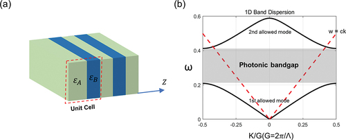
Electrons propagating inside a crystalline solid experience multiple bouncing and scatterings at interfaces. The overall complex interference allows the electrons to have only discrete momenta at a given frequency and yields an electronic band structure. The similarity between Schrödinger’s equation in quantum mechanics and the wave equation of light from Maxwell’s equations provides a photonic analogy to a crystalline solid. This so-called photonic crystal is an artificially engineered periodic structure composed of materials that have different refractive indices (Figure 1(a)). The spatial period $\mathrm{\Lambda }$ of the stack is called the lattice constant and is one of the major factors that determine the band properties of photonic crystals. Within photonic crystals, photons behave as electrons do in crystalline solids, and photons’ information, such as phase and group velocities, or allowed and prohibited spectral regions, can be described in terms of photonic band structure (Figure 1(b)). The energy dispersion of photons in free space is called the ‘light line’ or ‘light cone’ (Figure 1(b), red dashed line). This line distinguishes the region of the guided mode (under the light line) where the modes are confined to the slab and radiation modes (above the light line) where the mode can be coupled to the air. In addition, two modes have both positive and negative group velocities that refer to the existence of a back-propagation channel. This bidirectional propagation of photons in guiding induces light loss as known as back-scattering loss [33].

Figure 1. Schematic representation of 1D Photonic crystal and its band structure. (a) 1D photonic crystal composed of two alternating dielectric slabs with dielectric constant ϵ_A, ϵ_B with a period Λ. (b) Dispersion relation of 1D photonic crystal with two allowed modes. The 1st allowed mode is separated from the 2nd allowed mode by a photonic bandgap, which is a frequency regime in which the photon is not allowed to propagate. The red dashed line refers to the photon energy dispersion in free space that is called a light line. It divides the eigenmodes of a photonic crystal into bounded modes and radiative modes.

2.2 Topological photonic crystals

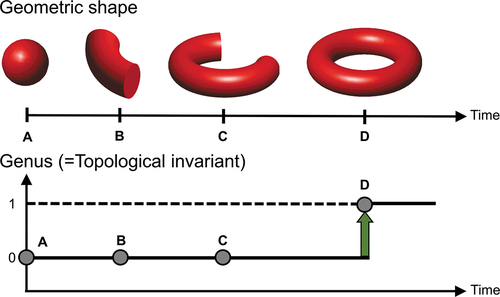
A photonic band has another hidden characteristic related to topology. Topology is a branch of mathematics that examines the geometric class of manifolds. An arbitrary manifold can be classified by topological invariants (usually integer-valued) which are conserved and quantized under continuous deformation. Figure 2 shows the adiabatic transformation of a manifold in time. If we consider the topological invariant as the number of holes, i.e. genus, then the four different states of the manifold at time A, B, and C have the same topological invariant which is zero. At this point, we can say that the three states are topologically equivalent even though they have different geometric shapes. On the other hand, the topological invariant of geometry D is not zero, which is different from states A, B, and C. It implies that the state D is topologically different from the states A, B, and C, that is, the adiabatic process from C to D does not preserve the number of holes. This discretized transformation is called a topological phase transition (green arrow). Those topological pictures can be applied in various fields of science and extend our understanding of the phase of matter.

Figure 2. Schematic illustration of topological phase transition of a manifold over time. The manifold at time A, which has a sphere-like shape geometry, starts to undergo continuous geometrical deformation. In the process of A to C, their geometric shapes are deformed smoothly, and their genus remains the same. In the process of C to D, however, a discrete topological jump happens, which is called a topological phase transition.

The topological phase of the photonic crystals is determined by the global behavior of photonic bands in reciprocal space which can be mathematically expressed as a Chern number [30,34]:

$C=\frac{1}{2\pi }{\int \int ◯}_{BZ}\mathcal{F}\left(k\right)\cdot \mathrm{d}\mathbf{s}$

where $\mathcal{F}\left(k\right)=\mathrm{\nabla }\times ⟨iu\left(k\right)\left|{\mathrm{\nabla }}_k\right|u\left(k\right)⟩$ is the Berry curvature of the band dispersion in the Brillouin zone (BZ), and $u\left(k\right)$ is the Bloch wave function. A topological invariant can also be represented by various forms such as winding number, and Zak phase (for 1D case), and all those kinds of invariants are essentially the same in physical implication [35]. The material or synthetic crystal becomes topologically nontrivial if those topological quantities are not zero. One of the topological classes is a quantum Hall insulator that is an insulator in the bulk, but a conductor on the edge. It has a nonzero Chern number and the edge state appears on the interface between the quantum Hall insulator and topologically-trivial insulator. This topologically-formed edge state has unidirectional group velocity and is robust against the disorder unless perturbation is larger than the bandgap [1,36,37].

To understand the fundamentals of topological photonic crystals, we introduce an example of a simple 1D toy model, the SSH model [38–41]. This model consists of a poly-acetylene chain with two alternating different sites that have different hopping strengths $v$ (hopping within the unit cell) and $w$ (hopping between neighboring unit cells) (Figure 3(a)). A pair of neighboring sites is distorted by Peierls instability [42] and constitutes a sublattice of sites A and B. The tight-Hamiltonian of such a system is

$H=v\sum _{n=1}^N\left(\left|n,B\right.⟩\left.⟨n,A\right|+h.c.\right)+w\sum _{n=1}^N\left(\left|n+1,A\right.⟩\left.⟨n,B\right|+h.c.\right)$

Figure 3. (a) Schematic representation of SSH model. The dotted box denotes a unit cell composed of two different sites A and B. (b) Three bulk band diagrams of SSH model for different parameter cases, v < w (yellow-colored region), v = w and v > w. (c) The two eigenenergy spectrums of finite SSH chain with open boundary, plotted as a function of w (with a value of v fixed at 1) and v (with a value of w fixed at 1), respectively. The zero modes occur only in cases of v < w (yellow-colored region) which refers to a topologically non-trivial case.

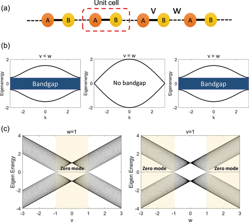
where $h.c.$ refers to the Hermitian conjugate of the term of preceding terms. Here we only consider nearest-neighbor interactions. The eigenenergy can be calculated using only v and w (Figure 3(b)).

Interestingly, although they seem to be perfectly symmetric for the case of $v>w$ and $v<w$ centered on the case of $v=w$, these two cases are topologically distinct. Consider the finite SSH model with an open boundary. Although their bulk spectra are the same, only the $v<w$ case (yellow-colored region) has a zero-energy mode (localized edge mode) (Figure 3(c)). This result occurs because this case is topologically non-trivial, i.e. their topological invariant is not zero. The topological properties of a bulk band are thus strongly coupled with the formation of localized modes. This kind of phenomenon is called ‘bulk-edge correspondence’ which means the topological non-triviality ensures the existence of a localized edge state [43].

Beyond such an aforementioned 1D system, numerous 2D and 3D topological photonic systems have also been studied [33,44–48]. The beginning of topological photonics considered the quantum Hall phase, which is composed of gyromagnetic materials that behave like electrons under a magnetic field [6]. The gyromagnetic coupling breaks the time-symmetry $\mathcal{T}$ and induces a nontrivial topological phase. However, for two fundamental reasons: i.e. (i) gyromagnetic effects are weak at the high-frequency regime and (ii) the difficulty in applying a strong magnetic field, other types of topological phases such as the quantum spin Hall phase [3] and quantum valley [10,49] Hall phase have begun to attract attention. The quantum spin Hall phase can be viewed as the sum of two independent quantum Hall phases, one for each spin degree of freedom of light. This phenomenon occurs because the Berry curvature is dependent on each spin, which corresponds to the circular polarization of electromagnetic waves. Recently, it has been found that the quantum valley Hall phase, which comes from the ‘valley’ degree of freedom, can replace the spin Hall phase in another way. In the valley Hall phase, the photons in a different valley propagate in the opposite direction; this phenomenon is called valley-momentum locking. The total Chern number of both quantum spin Hall and quantum valley Hall systems is zero, but the nonzero spin Chern number and nonzero valley Chern number provide a way to guide boundary states robustly.

Numerous other types of topological phases also exist, including Floquet topological phase [50–52], topological phase in the quasi-crystal [53–56], topological higher-order system [40,57], 3D topological Weyl photonic crystals [2,9,58–60]. We do not discuss these here because most studies on topological photonics with DL have considered a limited range of dimensionality and complexity such as simple SSH model [18,61] or Aubry–Andre–Harper model [62,63] or 1D photonic crystal [19,64,65]. Readers interested in other topological phases in more detail can refer to recent review papers [37,66,67].

3. Deep learning in nanophotonics

Inspired by human learning behavior, DL and overall machine learning algorithms use experience and sample data to learn the implicit rules of a system. These so-called training data are processed, analyzed and fitted to build an approximate model of a data-driven problem. For a given task, whether it is predicting certain values, making decisions, or even generating new samples, machine learning aims to construct a model capable of such a task without explicit human programming. Typical tasks of machine learning include regression, classification, clustering, and dimensionality-reduction of data space. Numerous algorithms are available for different problems.

Among various fields of machine learning, this review is focused on DL-based frameworks, a specific subfield, because most of the machine learning studies in nanophotonics have been carried out using DL techniques. DL is distinguished from other machine learning methods for using NN-based algorithm structures [20]. The most basic form of NN consists of layers of nodes, commonly called neurons, with nodes in each layer connected to nodes in the previous and subsequent layers; the connections are given weights that represent the strength of the influence of the sending node to the receiving node. The architecture resembles the complex interconnections of a brain’s neural system. A single neuron calculates an affine transformation of inputs according to the assigned weights and bias, then transfers the result to the next neuron through a nonlinear activation function (Figure 4(a)). When these neurons are assembled in a multilayered order (Figure 4(b)), and with well-trained weights, the collective effect of this whole structure enables the network to function as an approximate model that is capable of performing the desired task. The notion of the term ‘deep’ in deep learning comes from the use of many-layered NNs; to date the number of layers can be up to a few hundred.

Figure 4. Schematic illustration of a neural network (NN). (a) A single neuron calculates a weighted sum of inputs and adds a bias term, followed by a nonlinear activation function. The output value is passed as an input to the next layer. (b) A fully-connected, multiple layered NN. When an NN is properly trained, it learns the generalized, nonlinear relationship between the input (blue nodes) and the output (yellow nodes). (c) Schematic of NN training. The gradient of the loss function L with respect to each weight and bias value is calculated using the backpropagation algorithm. The input data batch is passed forward and every partial derivative of the learnable parameters is calculated from back to front. The weights are updated by the gradient descent rule with a defined learning rate α iteratively. The weight w_ij represents the j^th weight from the i^th layer to the next.

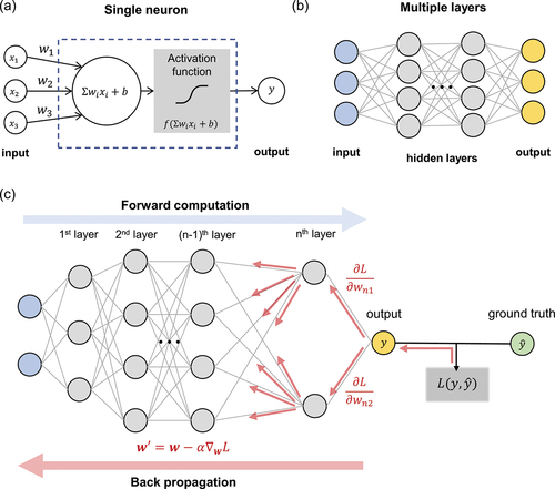
To train an NN, a loss function must be defined first. A loss function is a function that quantifies the difference between the desired output (ground truth) and the output produced by the NN model. Depending on the type of the desired task, an appropriate loss function should be chosen and adapted. Commonly used loss functions include the mean squared error for regression problems and the cross-entropy loss for classification problems. The weights of the NN are then adjusted to minimize this distance by using the gradient descent rule with an algorithm called backpropagation [68] (Figure 4(c)). In every iteration of forward passing of input data batch, it computes the gradient of the loss function with respect to each weight and bias using a chain rule, from the end of the NN to the front. The weights are then updated through iterations of gradient descent with a user-defined hyperparameter called the learning rate that determines the step size of each iteration.

Out of various classes of NNs, here we explain the two most basic forms, the fully-connected neural network (FCN) and the convolutional neural network (CNN). An FCN is a multiple-layer form, with each neuron being connected to all of the neurons in the next layer. Weights of FCN are assigned to every connection in the network. In contrast, a CNN [69] is typically characterized by its fundamental component, the convolutional layer, which performs convolution with specified kernels on inputs. These kernels, sometimes called filters, slide along the input features and perform elementwise products and summations, and the results are fed into a nonlinear activation function. Kernel values are learnable parameters which, after training, can extract spatially-local features of the input [70]. Because of these characteristics, CNN has shown remarkable results in analyzing image-like data to capture implicit spatial key features.

Physical values in nanophotonics were accurately discretized and formulated into different data-structures to implement DL algorithms [71]. Physical variables that describe nanostructures have been represented using a number of geometric parameters such as height, width, and periodicity. Materials were described with permittivity, permeability, or index values. Freeform 2D geometry structures were modeled as image data which can be well processed by CNN. Corresponding physical responses such as optical spectra, band structures, field distribution, or scattering patterns were discretized to a certain number of points to be appropriate to be input to, or output from, NNs.

Training an NN is an intricate process; it requires a careful formulation of the loss function depending on the desired task and an appropriate selection of a network model with correct hyperparameters, sometimes needing an extensive optimization process to be properly tuned [72,73]. Furthermore, to avoid overfitting, various training techniques such as cross-validation, regularization, dropout, or early stopping should be applied [74–78]. Most importantly, a large amount of good-quality training datasets must be prepared. This includes collecting and generating samples with proper labeling, normalization, or standardization. These mass data describing nanostructures and their corresponding physical responses are not usually available at hand, and therefore should be made specifically for the desired task using various electromagnetic simulation tools, which can take up a considerable amount of time.

DL applications in nanophotonics fall broadly into two categories: forward modeling and inverse design. Forward modeling in nanophotonics is a method to predict the optical properties of a given photonic structure design. Numerous studies have shown NNs can be remarkably well-trained to predict optical responses from various structure designs with reasonably accurate precision [79–95]. Inverse design is a method to find the photonic structure that has user-demanded optical responses. The ability of DL to capture nonlinear physical relationships was developed into various data-driven design methods that aimed to produce efficient and effective design frameworks that can directly achieve the desired objective of a device [71,96–100]. In this section, we will review DL applications in nanophotonics in forward modeling and inverse design. We will describe the overall goals and methods of DL frameworks and provide research examples that demonstrate the power of data-driven modeling.

3.1 Forward modeling

To solve a forward modeling problem, conventional approaches explicitly solve Maxwell’s equations analytically or numerically. Such methods provide near-exact, reasonable solutions calculated using physical laws, but practical constraints impede actual applications. For example, analytic or semi-analytic methods such as the transfer-matrix method and rigorous coupled-wave analysis become difficult to use in complex 3D problems in which structures have an arbitrary form. Numerical simulations, such as finite-difference time-domain and finite-element methods can solve such problems but have high computational costs. In comparison, if an NN is properly trained, it can provide a surrogate pathway that can evaluate the optical response of a complex structure orders-of-magnitude faster than a full-wave solver.

One pioneering example demonstrated the capability of the NN to learn the governing physical law in the study of scattering response of core-shell nanoparticles [79]. Peurifoy et al. used NNs to predict scattering cross-section spectra of SiO₂ and TiO₂ multilayer nanoparticles (Figure 5(a)). For the thickness of each shell given as inputs, the trained network could approximate light scattering with very high precision. Comparison between predictions from the NN and interior point method shows that the trained network is not just simply interpolating closest data points but capable of learning implicit rules of Maxwell interactions (Figure 5(b)).

Figure 5. Deep learning (DL) in nanophotonics. (a) Schematic of NN to predict the scattering cross-section of a core-shell nanoparticle [79]. The shell thickness and the scattering cross-section spectrum are used as training data. (b) Comparison of the approximated spectrum by NN to the simulated results, and closest data. (c) Schematics of forward model (left) and inverse model (right) [106]. The thickness of the multilayer structure and the transmission spectrum are used as training data. (d) Schematics of the SiO₂ and the Si₃N₄ multilayer structure and two designs that have the same transmission spectra. Figures adapted and reproduced from: (a, b) ref. [79], reproduced under a Creative Commons Attribution 4.0 International License (http://creativecommons.org/licenses/by/4.0) Copyright 2018, American Association for the Advancement of Science; (c, d) ref. [106], Copyright 2018, American Chemical Society.

NNs have also been demonstrated to predict other physical quantities of nanostructures such as different spectral responses, diffraction efficiencies, band structures, and Q factors. Examples include studies of ‘H-shaped’ plasmonic metasurfaces [80], chiral metamaterials [88–90], plasmonic absorbers [91], smart windows with phase-change materials [92], dielectric metasurfaces [93,94], dielectric metagratings [95] and photonic crystals [81–85]. Recent work has also developed a framework that can predict full near-field and far-field responses from arbitrary 3D structures [86]. This method has proven to be effective and extremely fast, so trained NN models are often used as surrogate forward solvers, to replace time-consuming simulation steps in the search for an optimal design [87,93,94].

Despite these remarkable results, implementing DL techniques is very tricky in practice because they are highly data-dependent. The prediction accuracy and the ability to learn the complex physical relationship without suffering from significant underfitting or overfitting relies heavily on training techniques and data quality. Generally, NNs can make reliable predictions for ranges within the boundaries of training data. If one wishes to train a network to work on a more generalized, wider range of design parameters, then the training data should be sufficiently diverse and large in amount accordingly. Sparse or biased data are major barriers in training a reliable NN model, so proper data collection and management are required and techniques such as data augmentation can further improve the training quality [101]. NN models have great potential for evaluating complex structures orders-of-magnitude faster compared to numerical simulations with just a one-time cost of training. However, this one-time cost involves the computational cost required for generating the training dataset and the training step itself. If a trained NN needs to be adapted to a new problem, for example, to problems with different kinds or number of input design variables, then the model will have to be retrained with a new set of training data which will have to be generated again. Studies on transfer learning which utilize the trained NN to solve a similar nanophotonic design problem [102] and unsupervised or semi-supervised learning algorithms requiring a small number of labeled data [103,104] show such burden of data collection can be mitigated for some level.

The unique advantage of NN models serving as highspeed function approximators within the predefined system is highly beneficial in design applications [81,82,87,93,94]. The early studies of forward predictions have provided useful insights of data-based modeling which led to subsequent advances in various systematic inverse design frameworks which are discussed in detail in the next section.

3.2 Inverse design

Unlike forward modeling where the output response of a certain input structure is always uniquely determined, for inverse design, there could be multiple structure candidates that show the same desired optical response. This one-to-many relationship makes the inverse problem more challenging. To handle such issues, attempts such as training multiple NNs [105] or training bidirectional networks that combine forward and inverse models have been made [80,88].

By using strategic frameworks, this problem can be better solved in a more stable manner. One approach is to pre-train the forward network, freeze its weights and then train the whole network with an inverse network combined at the front. This network architecture, generally called a tandem network, has been applied to designs with pre-set geometries [101,106–108]. Liu et al. showcased this scheme in designing a multilayer nanostructure of two different materials [106] (Figure 5(c),(d)). The non-uniqueness problem was solved by minimizing the error between the original input target spectrum and the forward network output spectrum. The tandem network was also shown to be capable of optimizing not just a few structure parameters but also of composing materials in a study of core-shell nanoparticles by successfully combining regression and classification problems in a single network [107].

While tandem networks can only be used in designs defined by several structural parameters, for arbitrary shapes, generative NNs capable of generating freeform devices can be used with conditional training. Generative models are NNs that can create a new sample from random noise in a probabilistic manner. This ability means that instead of direct discriminative modeling, such as straightforward prediction from target input to design output, the generative NN includes modeling of implicit probability distribution in the design framework. By doing so, generative models can perform probabilistic perturbation or sampling on the modeled distribution space and thereby introduce some degree of randomness in the design process. This approach can overcome the one-to-many mapping problem and propose a new, freeform design for a given conditional requirement (target input).

Among many classes of generative models, the variational autoencoder (VAE) [109] and generative adversarial networks (GAN) [110] are commonly adopted models. Application of VAE has been demonstrated in the design of double-layer chiral meta-atoms [111] and nanopatterned power splitters [112]. Various frameworks that use a conditional GAN have been developed to produce devices that have the desired spectrum [113,114]. In particular, recent research has proposed a wide variety of GAN-based inverse design methods coupled with other optimization techniques to get high-performing, near-globally-optimal devices [115,116] or to solve complex problems such as multi-objective tasks [117].

Other powerful computational methods including gradient-based optimization (e.g. topology optimization and adjoint method) and evolutionary algorithm-empowered searching methods (e.g. genetic algorithm and particle swarm optimization) are still actively used in nanophotonics as tools of inverse design [118]. The DL-based approach cannot fully replace these methods, but still have several profound, distinctive advantages. Computational methods rely heavily on iterations and updates with numerous steps of simulations and therefore can take large amounts of time and computer resources, so the step can be a major bottleneck in the design process. As the design complexity increases associated with increased dimension, enlarged device space, and multiple constraints, this problem becomes increasingly severe, because the number of iterations scales up dramatically, so the method is no longer applicable in practice. DL can alleviate such time-consuming steps and process highly complex designs by using various NN frameworks and data-engineering techniques. The use of DLs can be combined with other optimization methods to further improve the target device’s characteristics and function, or increase the efficiency of the design process.

4. Deep learning integrated topological photonics

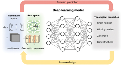
As this overview of DL-assisted nanophotonic studies shows, the key advantage of DL modeling is its ability to identify the highly non-linear relationship between data, and to enable the development of an approximating physical model. This ability enables us to manipulate and understand complex systems in ways that are otherwise impossible due to practical constraints. DL that has been performed on topological photonics can be classified into two main classes: (i) forward prediction of topological states (ii) inverse design of photonic systems for desired topological properties (Figure 6). The latter is distinguished from parametric regression where the parameters are determined by a predefined optimization function for fitting data. In contrast, with DL, by supervised learning, NNs can include the underlying physical mechanism in input data. In the following section, we will cover two main categories of recently-studied topological photonics with DL and their significance.

Figure 6. Schematic of DL application framework in topological systems. For forward prediction tasks, geometric or momentum space parameters are used as inputs, and the trained DL model predicts its corresponding topological properties. For inverse design tasks, desired topological properties are fed as inputs and the model outputs the design parameters that yield those properties.

4.1 Forward prediction of topological states

One of the most distinctive parts of DL models in topological systems is that the models are usually trained to predict discrete values, whereas many other problems in nanophotonics predict continuous spectra, such as transmission or scattering efficiencies, because one of the primary concerns in topological photonics is the identification and classification of topological fingerprints. In conventional approaches, the direct numerical or analytic calculation should be performed to get the topological parameter e.g. winding number, Chern number, Zak phase. Otherwise, the use of mathematical knowledge such as group theory or K-theory is a possible choice, but given the increasing complexity and dimensionality of the physical models of interest, detailed characterization towards the topological phase is becoming increasingly challenging.

Recently, various attempts to use DL to identify the topological phase of matter in condensed matter physics and photonics have been reported [18,65,119–122]. Unlike the conventional phase of matter, which is characterized by local order parameters that represent the degree of order such as magnetization and heat, the topological phase is dependent on the global appearance. Nevertheless, the NN can predict the ‘global’ property quite successfully with the ‘local’ features by using a supervised DL algorithm in a predefined topological model [18,61,65,119,120,123–125]. This success is astonishing because the network has no pre-information about how the topological parameter is to be determined, whereas previous work has solved the problem by defining a specific function or relying on the presence of topological edge states. Surprisingly, properly supervised NNs can identify a topological phase that is not included in the training dataset [18,61,65].

Zhang, et al. performed supervised training of a CNN to predict winding numbers beyond the training dataset with nearly 100% accuracy [18] (Figure 7(a)). The authors first trained the NNs with a 1D SSH model. When the test data set was restricted in the SSH model, their trained networks could compute winding numbers with nearly 100% accuracy. However, if test data included a more general form of Hamiltonian, accuracy was drastically decreased. This loss implies that the NNs trained for a certain model cannot exploit universal features of topology, so they find the shortcut of a simplified winding number formula that is only valid in that model. To overcome this limitation and to examine whether the NN is fully capable of predicting the winding number in any general cases, they produced training data with the most general form of Hamiltonian with chiral symmetry. Interestingly, CNN showed significantly better extrapolation accuracy than an FCN by successfully capturing the translation symmetry of lattice (Figure 7(b)).

Figure 7. Prediction of topological invariant using forward DL process. (a) Schematic of DL framework with CNN and FCN. Randomly-sampled Hamiltonians in momentum space are used as training data and the winding numbers are predicted [18]. (b) Accuracy of the CNN with respect to the regularization strength, which is used to avoid overfitting and to increase generalized prediction capability. Winding number with absolute value < 2 is in the training set, otherwise is not. (c) Schematic illustration of workflow to predict the topological invariants with physics-adapted NN and operator parameter space [65]. (d) The architecture of the NN consists of two convolution layers and linear layers (above) and the resulting phase diagram of breathing Kagome lattice with disorders for the rhombus and triangle geometry, respectively (below) [119]. The input image is the electron density of the highest occupied state. In the left plot, the blue, right-blue, yellow, and Orange areas represent trivial, HOTI 1, HOTI 2, and metallic phases. In the right plot, red, blue and green areas represent trivial, HOTI, and metallic phases Figures reproduced from: (a, b) ref. [18], Copyright 2018, American Physical Society; (c) ref. [65], Copyright 2020, American Physical Society; (d) ref. [119], Copyright 2019, American Physical Society.

However, the unbalance of complexity between training dataset and system leads to the failure of NNs to capture the generalized physical relationship. This problem is caused by a trade-off relation between system complexity and bias: as the system complexity increases the bias decreases and vice versa [126]. Therefore, for the NN to have extrapolation capability, the bias and variance must be optimally balanced. Wu et al. attempted to solve this problem by enlarging the training set [65]. The authors mitigated an additional parameter space that encodes physical laws (operator parameter space), then used it to produce a physics-adapted NN to improve the ability to predict topological transition beyond its training set (Figure 7(c)). When trained with an additional dataset of the physical parameters encoded with Maxwell equations, the NN’s prediction capability was significantly improved. The bias-variance trade-off relations showed that such enrichment in the input training set was balanced well with the complexity of the given system, and increased the NN’s prediction capability.

DL in forward prediction has also been effectively utilized in the presence of disorders [119,127–130]. In a disordered system, in a higher-ordered topological insulator (HOTI) where topological boundary modes have lower dimensions than modes of bulk, the criterion to distinguish the topological phases is ambiguous; HOTI phases cannot be identified only by the topological indices and also their robustness against disorders is unclear [119]. However, DL successfully calculated the phase diagram of HOTI in the disordered system by checking the presence of survived localized corner states, and also confirmed their robustness. Araki et al. used DL to predict the phase diagram of a HOTI by the existence of the corner states in a breathing Kagome lattice in the different hopping-parameter ratios. The prediction framework using CNN was trained with the electron density of the highest occupied single particle as an input/output vector. The authors introduced an on-site random potential $H^{\mathrm{\prime }}=\sum _i{w}_i{c}_i^{†}{c}_i$ to consider disorder, where $w_i$ are randomly-distributed values. The retrieved phase diagram of rhombus and triangular geometries shows that the NN can distinguish the HOTI phases well (Figure 7(d)). In addition, by conducting a parameter study, they found that the HOTI phase is unaffected by disorder as long as the disorder perturbation strength is smaller than the energy gap. Although this study was conducted in an electronic system, it is also sufficiently applicable in photonics.

These attempts to use DL to obtain forward prediction of topological fingerprints demonstrate that the NN can capture the inherent physics of defining topological invariants within the training dataset. This ability suggests the possibility that DL could contribute to theoretical investigation to find exotic topological physics. Although such findings have not yet been made, they are worth anticipating, considering that topological photonics with DL is in its early stages.

4.2 Inverse design of topological systems

Ongoing studies offer novel prospects of topological photonics such as topological lasers and advanced integrated photonic circuits [131–135]. However, how to engineer a physical system to have topological properties for a specific application remains a challenging question. The relationship between real space design parameters and topological behaviors is highly non-linear and non-intuitive, so in practice engineers typically resort to repetitive trials with analytical or numerical forward computations [132,133,135]. Inverse design using DL aims to systematically reduce this computational load by developing an approximate data-driven inverse model.

For example, Pilozzi et al. demonstrated a method for identifying the design parameters of a 1D Aubry-Andre-Harper topological insulator to obtain protected edge states at target frequencies [63]. The proposed NN used both the inverse network and the forward network together (Figure 8(a)). When the target edge state frequency is fed as input, the inverse network outputs the design parameter, which is then used as input for the forward network. This scheme was to ensure that the obtained solution was indeed physically viable by comparing the final output of the forward network with the original target input. The solution was rejected if this difference was above a threshold. The additional problem of multivalued degeneracy in the forward problem was solved by introducing categorical variables that specified the eigenmode and domains of frequency as additional input features. Further, discontinuity of domain was treated by training multiple, independent NNs for each continuous range. It successfully solved both forward and inverse problems (Figure 8(b)).

Figure 8. Inverse design of topological systems using DL. (a) The forward and inverse networks used to find the specific edge state frequency. (b) Forward problem and inverse problem reconstruction of edge-states dispersion by DL models [63]. (c) Schematic of bandgap modeling of multilayer PCs represented as label vector. (d) Comparison of target label vector and obtained label vector from proposed framework [19]. Figures reproduced from: (a, b) ref. [63], reproduced under a Creative Commons Attribution 4.0 International License (http://creativecommons.org/licenses/by/4.0) Copyright 2018, Springer Nature. (c, d) ref. [19], Copyright 2019, American Institute of Physics Publishing Group.

The above example treated the one-to-many mapping problem by imposing additional constraints or variables indicating a specific range of the target response. Also, checking each solution’s valid regime in a case-by-case manner was required. This cumbersome process can be alleviated by using a tandem network. Long et al. showcased an example of obtaining geometrical parameters of 1D photonic crystals for the desired Zak phase property [19] (Figure 8(c)). The NN was pretrained with a forward relationship from the length of each layer in the unit cell to the signs of the reflection phases of bandgaps. Following the generic tandem framework scheme, the inverse network was then combined at the front and trained again. The target topological property and obtained topological property from the inverse designed devices showed excellent agreement (Figure 8(d)). A tandem network has also been used to design topological states of 1D photonic crystals by Singh et al [64].; the thicknesses of periodic layers were set as design parameters, and the bandgap structures were set as device properties. The retrieved bandgap structure matched perfectly with the target bandgap values, and thereby proved the efficacy of the proposed method.

5. Summary and outlook

In this review, we have provided examples of topological photonics merged with DL. Various supervised learning strategies have demonstrated DL’s generalization ability to extrapolate physical values beyond the training dataset. Trained models could accurately predict topological invariants such as winding numbers, or classify topological phases of a given system by using only local features. An interesting outlook of how DL can provide insights to understand complex topological phenomena using data-generated physical models was also suggested. In addition, DL is a powerful inverse design tool, so various design strategies have been proposed, to manipulate topologically nontrivial systems to have desired optical properties.

Although the scope of this review is limited to DL applications with NNs, most of them using supervised learning strategy, there are other machine learning techniques beyond NNs that are actively studied for enhanced analysis of topological systems. Recent works have demonstrated persistent homology [136] and various unsupervised learning strategies such as diffusion map [137] based manifold learning methods [138–140] and clustering algorithms with topological data analysis [141] to effectively identify the topological features by direct inspection from data. Unsupervised learning techniques, in particular, are advantageous in that it learns from label-free data and can capture various notions of similarity between phases in dimension-reduced parameter space. These works show the power of data-driven methods enabling a high-throughput classification of topological states and the potential to detect topological properties from various structures without relying on a priori knowledge.

Indeed, although the two independent research fields, topological photonics and DL, have made revolutionary advances in parallel, the combination of the two has so far only been tested using simple models and algorithms. However, we stress the importance of the continuous effort to combined the two disciplines. Materials with novel properties are being sought, to enable next-generation optical technology. Topological photonics, in particular, is attracting considerable attention for its potential to realize a highly robust transmission immune to defects and disorders. To tailor such behavior for a specific need, effective modeling methods must be uncovered. The non-local nature of a topological property requires a global inspection of the whole system, and this process becomes unmanageable as the system dimension and complexity expand. To solve this problem, the adoption of DL is essential: data-driven models can process models, despite the increasing complexity of physical systems.

The need to adopt DL in topological photonics is not limited to the effective modeling of complex systems and design applications. An emerging research field called ‘explainable artificial intelligence’ seeks methods to enable DL models to provide results that are understandable to experts in the domain [142]. Research in this field aims to elucidate the black-box nature of data-driven models and thereby is expected to provide physically valuable insights. Such movement has already emerged in areas of nanophotonics [143] and material science [144] including those related to topological properties [61]. Model explainability can be achieved with extensive data analysis empowered by DL, and explainable models are expected to be important tools for investigation in general physics.

From fundamentals to application, topological photonics integrated with DL have important potential. Physical models obtained using DL will advance the understanding of topological systems beyond our current theoretical background. We envision that data-driven methods will become increasingly well-established, and will be extended to be able to design complex 2D to 3D topological structures by adopting higher-level DL algorithms. This combined research will certainly provide invaluable insights in photonics, physics, material science, and their interdisciplinary areas.

Disclosure statement

No potential conflict of interest was reported by the author(s).

Additional information

Funding

This work was financially supported by the POSCO-POSTECH-RIST Convergence Research Center program funded by POSCO, and the National Research Foundation (NRF) grants (NRF-2019R1A2C3003129, CAMM-2019M3A6B3030637, NRF-2019R1A5A8080290) funded by the Ministry of Science and ICT (MSIT) of the Korean government. S.S. and M.K. acknowledge the NRF Sejong Science fellowships (NRF-2022R1C1C2009430 & NRF-2022R1C1C2004662), respectively, funded by the MSIT of the Korean government. S.S. acknowledges the Institute of Information & Communications Technology Planning & Evaluation (IITP) grant (No.2019-0-01906, POSTECH Artificial Intelligence Graduate School Program) funded by the MSIT of the Korean government.

References

- Raghu S, Haldane FDM. Analogs of quantum-hall-effect edge states in photonic crystals. Phys Rev A. 2008;78:033834.
- Lu L, Fu L, Joannopoulos JD, et al. Weyl points and line nodes in gyroid photonic crystals. Nat Photonics. 2013;7:294–29.
- Bliokh KY, Smirnova D, Nori F. Quantum spin hall effect of light. Science. 2015;348:1448–1451.
- Yang Z, Gao F, Shi X, et al. Topological acoustics. Phys Rev Lett. 2015;114:114301.
- Krishnamoorthy HNS, Jacob Z, Narimanov E, et al. Topological transitions in metamaterials. Science. 2012;336:205–209.
- Wang Z, Chong YD, Joannopoulos JD, et al. Reflection-free one-way edge modes in a gyromagnetic photonic crystal. Phys Rev Lett. 2008;100:013905.
- Kane CL, Mele EJ. Z2 topological order and the quantum spin hall effect. Phys Rev Lett. 2005;95:146802.
- Hafezi M, Mittal S, Fan J, et al. Imaging topological edge states in silicon photonics. Nat Photonics. 2013;7:1001–1005.
- Lu L, Wang Z, Ye D, et al. Experimental observation of weyl points. Science. 2015;349:622–624.
- Ma T, Shvets G. All-Si valley-hall photonic topological insulator. New J Phys. 2016;18:025012.
- Yang B, Guo Q, Tremain B, et al. Direct observation of topological surface-state arcs in photonic metamaterials. Nat Commun. 2017;8:97.
- Kim M, Lee D, Lee D, et al. Topologically nontrivial photonic nodal surface in a photonic metamaterial. Phys Rev B. 2019;99:235423.
- Guo Q, Yang B, Xia L, et al. Three dimensional photonic dirac points in metamaterials. Phys Rev Lett. 2017;119:213901.
- Kim M, Gao W, Lee D, et al. Extremely broadband topological surface states in a photonic topological metamaterial. Adv Opt Mater. 2019;7:1900900.
- Hafezi M, Demler EA, Lukin MD, et al. Robust optical delay lines with topological protection. Nat Phys. 2011;7:907–912.
- Yang Y, Yamagami Y, Yu X, et al. Terahertz topological photonics for on-chip communication. Nat Photonics. 2020;14:446–451.
- Barik S, Karasahin A, Flower C, et al. A topological quantum optics interface. Science. 2018;359:666–668.
- Zhang P, Shen H, Zhai H. Machine learning topological invariants with neural networks. Phys Rev Lett. 2018;120:66401.
- Long Y, Ren J, Li Y, et al. Inverse design of photonic topological state via machine learning. Appl Phys Lett. 2019;114:181105.
- LeCun Y, Bengio Y, Hinton G. Deep learning. Nature. 2015;521:436–444.
- Jordan MI, Mitchell TM. Machine learning: trends, perspectives, and prospects. Science. 2015;349:255–260.
- Krizhevsky A, Sutskever I, Hinton GE. ImageNet classification with deep convolutional neural networks. Advances in Neural Information Processing Systems. Lake Tahoe, Nevada. 2012;25:1097–1105.
- Deng L, Li X. Machine learning paradigms for speech recognition: an overview. IEEE Trans Audio Speech Lang Process. 2013;21:1060–1089.
- Shalev-Shwartz S, Shammah S, Shashua AS. Safe, multi-agent, reinforcement learning for autonomous driving. arXiv:1610.03295 [cs.AI]. 2016.
- Silver D, Huang A, Maddison CJ, et al. Mastering the game of go with deep neural networks and tree search. Nature. 2016;529:484–489.
- Benjamin S-L, Alán A-G. Inverse molecular design using machine learning: generative models for matter engineering. Science. 2018;361:360–365.
- Goh GB, Hodas NO, Vishnu A. Deep learning for computational chemistry. J Comput Chem. 2017;38:1291–1307.
- Baldi P, Sadowski P, Whiteson D. Searching for exotic particles in high-energy physics with deep learning. Nat Commun. 2014;5:4308.
- Klitzing KV, Dorda G, Pepper M. New method for high-accuracy determination of the fine-structure constant based on quantized hall resistance. Phys Rev Lett. 1980;45:494–497.
- Thouless DJ, Kohmoto M, Nightingale MP, et al. Quantized hall conductance in a two-dimensional periodic potential. Phys Rev Lett. 1982;49:405–408.
- Lu J, Qiu C, Deng W, et al. Valley topological phases in bilayer sonic crystals. Phys Rev Lett. 2018;120:116802.
- Huber SD. Topological mechanics. Nat Phys. 2016;12:621–623.
- Wang Z, Chong Y, Joannopoulos JD, et al. Observation of unidirectional backscattering-immune topological electromagnetic states. Nature. 2009;461:772–775.
- Kohmoto M. Topological invariant and the quantization of the hall conductance. Ann Phys. 1985;160:343–354.
- Ando Y. Topological Insulator Materials. J Phys Soc Jap. 2013;82:102001.
- Haldane FDM, Raghu S. Possible Realization of Directional Optical Waveguides in Photonic Crystals with Broken Time-Reversal Symmetry. Phys Rev Lett. 2008;100:013904.
- Ozawa T, Price HM, Amo A, et al. Topological photonics. Rev Mod Phys. 2019;91:015006.
- Su WP, Schrieffer JR, Heeger AJ. Solitons in polyacetylene. Phys Rev Lett. 1979;42:1698–1701.
- Malkova N, Hromada I, Wang X, et al. Observation of optical shockley-like surface states in photonic superlattices. Opt Lett. 2009;34:1633–1635.
- El Hassan A, Kunst FK, Moritz A, et al. Corner states of light in photonic waveguides. Nat Photonics. 2019;13:697–700.
- Kim M, Rho J. Topological edge and corner states in a two-dimensional photonic su-schrieffer-heeger lattice. Nanophotonics. 2020;9:3227–3234.
- Batra N, Sheet G. Physics with coffee and doughnuts. Resonance. 2020;25:765–786.
- Rudner MS, Lindner NH, Berg E, et al. Anomalous edge states and the bulk-edge correspondence for periodically driven two-dimensional systems. Phys Rev X. 2013;3:031005.
- Poo Y, Wu R, Lin Z, et al. Experimental realization of self-guiding unidirectional electromagnetic edge states. Phys Rev Lett. 2011;106:093903.
- Cheng X, Jouvaud C, Ni X, et al. Robust reconfigurable electromagnetic pathways within a photonic topological insulator. Nat Mater. 2016;15:542–548.
- Slobozhanyuk A, Mousavi SH, Ni X, et al. Three-dimensional all-dielectric photonic topological insulator. Nat Photonics. 2017;11:130–136.
- Yang Y, Gao Z, Xue H, et al. Realization of a three-dimensional photonic topological insulator. Nature. 2019;565:622–626.
- Wu L-H, Hu X. Scheme for achieving a topological photonic crystal by using dielectric material. Phys Rev Lett. 2015;114:223901.
- Kim M, Kim Y, Rho J. Spin-valley locked topological edge states in a staggered chiral photonic crystal. New J Phys. 2020;22:113022.
- Maczewsky LJ, Zeuner JM, Nolte S, et al. Observation of photonic anomalous floquet topological insulators. Nat Commun. 2017;8:13756.
- Rechtsman MC, Zeuner JM, Plotnik Y, et al. Photonic floquet topological insulators. Nature. 2013;496:196–200.
- Lindner NH, Refael G, Galitski V. Floquet topological insulator in semiconductor quantum wells. Nat Phys. 2011;7:490–495.
- Verbin M, Zilberberg O, Kraus YE, et al. Observation of topological phase transitions in photonic quasicrystals. Phys Rev Lett. 2013;110:076403.
- Aubry S,André G. Analyticity breaking and Anderson localization in incommensurate lattices. Ann Isr Phys Soc. 1980;3:133.
- Levine D, Steinhardt PJ. Quasicrystals: a new class of ordered structures. Phys Rev Lett. 1984;53:2477–2480.
- Kraus YE, Lahini Y, Ringel Z, et al. Topological states and adiabatic pumping in quasicrystals. Phys Rev Lett. 2012;109:106402.
- Noh J, Benalcazar WA, Huang S, et al. Topological protection of photonic mid-gap defect modes. Nat Photonics. 2018;12:408–415.
- Lin Q, Xiao M, Yuan L, et al. Photonic weyl point in a two-dimensional resonator lattice with a synthetic frequency dimension. Nat Commun. 2016;7:13731.
- Chen WJ, Xiao M, Chan CT. Photonic crystals possessing multiple weyl points and the experimental observation of robust surface states. Nat Commun. 2016;7:13038.
- Yang B, Guo Q, Tremain B, et al. Ideal weyl points and helicoid surface states in artificial photonic crystal structures. Science. 2018;359:1013–1016.
- Holanda NL,Griffith MAR. Machine learning topological phases in real space. Phys Rev B. 2020;102:054107.
- Pilozzi L, Farrelly FA, Marcucci G, et al. Topological nanophotonics and artificial neural networks. Nanotechnology. 2021;32:142001.
- Pilozzi L, Farrelly FA, Marcucci G, et al. Machine learning inverse problem for topological photonics. Commun Phys. 2018;1:57.
- Singh R, Agarwal A, Anthony W. Mapping the design space of photonic topological states via deep learning. Opt Express. 2020;28:27893–27902.
- Wu B, Ding K, Chan CT, et al. Machine prediction of topological transitions in photonic crystals. Phys Rev Appl. 2020;14:044032 .
- Kim M, Jacob Z, Rho J. Recent advances in 2D, 3D and higher-order topological photonics. Light Sci Appl. 2020;9:130.
- Lu L, Joannopoulos JD, Soljačić M. Topological photonics. Nat Photonics. 2014;8:821–829.
- Rumelhart DE, Hinton GE, Williams RJ. Learning representations by back-propagating errors. Nature. 1986;323:533–536.
- Lawrence S, Giles CL, Tsoi AC, et al. Face recognition: a convolutional neural-network approach. IEEE Trans Neural Networks. 1997;8:98–113.
- Simonyan K, Zisserman A. Very deep convolutional networks for large-scale image recognition. arXiv:1409.1566 [cs.CV]. 2014.
- Jiang J, Chen M, Fan JA. Deep neural networks for the evaluation and design of photonic devices. Nat Rev Mater. 2021;6:679–700.
- Snoek J, Larochelle H, Adams RP. Practical bayesian optimization of machine learning algorithms. Advances in Neural Information Processing Systems. Lake Tahoe, Nevada. 2012;25:2951–2959.
- Bergstra J, Bengio Y. Random search for hyper-parameter optimization. J Mach Learn Res. 2012;13:281–305.
- Kohavi R. A study of cross-validation and bootstrap for accuracy estimation and model selection. Proceedings of the 14th international joint conference on Artificial intelligence. San Francisco, CA, USA. 1995;2:1137–1143.
- Bengio Y. No unbiased estimator of the variance of k-fold cross-validation. J Mach Learn Res. 2004;5:1089–1105.
- Hinton G. Dropout : a simple way to prevent neural networks from overfitting. J Mach Learn Res. 2014;15:1929–1958.
- Caruana R, Lawrence S, Giles C. Overfitting in neural nets: backpropagation, conjugate gradient, and early stopping. Advances in Neural Information Processing Systems. Denver, CO, USA. 2000;13:402–408.
- Goodfellow I, Bengio Y, Courville A. Regularization for Deep Learning. In: Deep Learning. Cambridge, MA, USA: MIT press; 2016; p. 224–270.
- Peurifoy J, Shen Y, Jing L, et al. Nanophotonic particle simulation and inverse design using artificial neural networks. Sci Adv. 2018;4:eaar4206.
- Malkiel I, Mrejen M, Nagler A, et al. Plasmonic nanostructure design and characterization via deep learning. Light Sci Appl. 2018;7:60.
- Asano T, Noda S. Iterative optimization of photonic crystal nanocavity designs by using deep neural networks. Nanophotonics. 2019;8:2243–2256.
- Christensen T, Loh C, Picek S, et al. Predictive and generative machine learning models for photonic crystals. Nanophotonics. 2020;9:4183–4192.
- Da Silva Ferreira A, Malheiros-Silveira GN, Hernandez-Figueroa HE. Computing optical properties of photonic crystals by using multilayer perceptron and extreme learning machine. J Light Technol. 2018;36:4066–4073.
- Chugh S, Gulistan A, Ghosh S, et al. Machine learning approach for computing optical properties of a photonic crystal fiber. Opt Express. 2019;27:36414–36425.
- Asano T, Noda S. Optimization of photonic crystal nanocavities based on deep learning. Opt Express. 2018;26:32704–32717.
- Wiecha PR, Muskens OL. Deep learning meets nanophotonics: a generalized accurate predictor for near fields and far fields of arbitrary 3d nanostructures. Nano Lett. 2020;20:329–338.
- Kudyshev ZA, Kildishev AV, Shalaev VM, et al. Machine learning–assisted global optimization of photonic devices. Nanophotonics. 2020;10:371–383.
- Ma W, Cheng F, Liu Y. Deep-learning-enabled on-demand design of chiral metamaterials. ACS Nano. 2018;12:6326–6334.
- Li Y, Xu Y, Jiang M, et al. Self-learning perfect optical chirality via a deep neural network. Phys Rev Lett. 2019;123:213902.
- Tao Z, Zhang J, You J, et al. Exploiting deep learning network in optical chirality tuning and manipulation of diffractive chiral metamaterials. Nanophotonics. 2020;9:2945–2956.
- Sajedian I, Kim J, Rho J. Finding the optical properties of plasmonic structures by image processing using a combination of convolutional neural networks and recurrent neural networks. Microsyst Nanoeng. 2019;5:27.
- Balin I, Garmider V, Long Y, et al. Training artificial neural network for optimization of nanostructured VO 2 -based smart window performance. Opt Express. 2019;27:A1030–A1040.
- Nadell CC, Huang B, Malof JM, et al. Deep learning for accelerated all-dielectric metasurface design. Opt Express. 2019;27:27523–27535.
- An S, Fowler C, Zheng B, et al. A deep learning approach for objective-driven all-dielectric metasurface design. ACS Photonics. 2019;6:3196–3207.
- Inampudi S, Mosallaei H. Neural network based design of metagratings. Appl Phys Lett. 2018;112:241102.
- So S, Badloe T, Noh J, et al. Deep learning enabled inverse design in nanophotonics. Nanophotonics. 2020;9:1041–1057.
- Ma W, Liu Z, Kudyshev ZA, et al. Deep learning for the design of photonic structures. Nat Photonics. 2021;15:77–90.
- Xu Y, Zhang X, Fu Y, et al. Interfacing photonics with artificial intelligence: an innovative design strategy for photonic structures and devices based on artificial neural networks. Photonics Res. 2021;9:B135–B152.
- Liu Z, Zhu D, Raju L, et al. Tackling photonic inverse design with machine learning. Adv Sci. 2021;8:2002923.
- So S, Lee D, Badloe T, et al. Inverse design of ultra-narrowband selective thermal emitters designed by artificial neural networks. Opt Mater Express. 2021;11:1863–1873.
- Noh J, Nam YH, So S, et al. Design of a transmissive metasurface antenna using deep neural networks. Opt Mater Express. 2021;11:2310–2317.
- Qu Y, Jing L, Shen Y, et al. Migrating knowledge between physical scenarios based on artificial neural networks. ACS Photonics. 2019;6:1168–1174.
- Ma W, Liu Y. A data-efficient self-supervised deep learning model for design and characterization of nanophotonic structures. Sci China Phys Mech Astron. 2020;63:284212.
- Trivedi R, Su L, Lu J, et al. Data-driven acceleration of photonic simulations. Sci Rep. 2019;9:19728.
- Baxter J, Calà Lesina A, Guay JM, et al. Plasmonic colours predicted by deep learning. Sci Rep. 2019;9:8074.
- Liu D, Tan Y, Khoram E, et al. Training deep neural networks for the inverse design of nanophotonic structures. ACS Photonics. 2018;5:1365–1369.
- So S, Mun J, Rho J. Simultaneous inverse design of materials and structures via deep learning: demonstration of dipole resonance engineering using core-shell nanoparticles. ACS Appl Mater Interfaces. 2019;11:24264–24268.
- So S, Yang Y, Lee T, et al. On-demand design of spectrally sensitive multiband absorbers using an artificial neural network. Photonics Res. 2021;9:B153–B158.
- Kingma DP, Welling M. Auto-encoding variational bayes. arXiv:1312.6114[stat.ML]. 2013.
- Goodfellow I, Pouget-Abadie J, Mirza M. Generative adversarial nets. In: Advances in Neural Information Processing Systems. Montreal, Canada. 2014;27:2672–2680.
- Ma W, Cheng F, Xu Y, et al. Probabilistic representation and inverse design of metamaterials based on a deep generative model with semi-supervised learning strategy. Adv Mater. 2019;31:1901111.
- Tang Y, Kojima K, Koike‐Akino T, et al. Generative deep learning model for inverse design of integrated nanophotonic devices. Laser Photonics Rev. 2020;14:2000287.
- Liu Z, Zhu D, Rodrigues SP, et al. Generative model for the inverse design of metasurfaces. Nano Lett. 2018;18:6570–6576.
- So S, Rho J. Designing nanophotonic structures using conditional deep convolutional generative adversarial networks. Nanophotonics. 2019;8:1255–1261.
- Jiang J, Sell D, Hoyer S, et al. Free-form diffractive metagrating design based on generative adversarial networks. ACS Nano. 2019;13:8872–8878.
- Jiang J, Fan JA. Global optimization of dielectric metasurfaces using a physics-driven neural network. Nano Lett. 2019;19:5366–5372.
- Jiang J, Fan JA. Multiobjective and categorical global optimization of photonic structures based on resNet generative neural networks. Nanophotonics. 2020;10:361–369.
- Molesky S, Lin Z, Piggott AY, et al. Inverse design in nanophotonics. Nat Photonics. 2018;12:659–670.
- Araki H, Mizoguchi T, Hatsugai Y. Phase diagram of a disordered higher-order topological insulator: a machine learning study. Phys Rev B. 2019;99:085406.
- Sun N, Yi J, Zhang P, et al. Deep learning topological invariants of band insulators. Phys Rev B. 2018;98:085402.
- Zhang Y, Kim EA. Quantum loop topography for machine learning. Phys Rev Lett. 2017;118:216401.
- Deng DL, Li X, Das Sarma S. Machine learning topological states. Phys Rev B. 2017;96:195145.
- Carrasquilla J. Neural networks identify topological phases. Physics. 2017;10:56.
- Peano V, Sapper F, Marquardt F. Rapid exploration of topological band structures using deep learning. Phys Rev X. 2021;11:021052.
- Ming Y, Lin CT, Bartlett SD, et al. Quantum topology identification with deep neural networks and quantum walks. npj Comput Mater. 2019;5:88.
- Mehta P, Wang CH, Day AGR, et al. A high-bias, low-variance introduction to machine learning for physicists. Phys Rep. 2019;810:1–124.
- Yoshioka N, Akagi Y, Katsura H. Learning disordered topological phases by statistical recovery of symmetry. Phys Rev B. 2018;97:205110.
- Yu S, Piao X, Park N. Machine learning identifies scale-free properties in disordered materials. Nat Commun. 2020;11:4842.
- Cubuk ED, Schoenholz SS, Rieser JM, et al. Identifying structural flow defects in disordered solids using machine-learning methods. Phys Rev Lett. 2015;114:108001.
- Fujii K, Nakajima K. Harnessing disordered-ensemble quantum dynamics for machine learning. Phys Rev Appl. 2017;8:024030.
- Zhao H, Qiao X, Wu T, et al. Non-Hermitian topological light steering. Science. 2019;365:1163–1166.
- Ota Y, Katsumi R, and Watanabe K, et al. Topological photonic crystal nanocavity laser. Commun Phys. 2018;1:86.
- Shao ZK, Chen HZ, Wang S, et al. A high-performance topological bulk laser based on band-inversion-induced reflection. Nat Nanotechnol. 2020;15:67–72.
- Ma J, Xi X, Sun X. Topological photonic integrated circuits based on valley kink states. Laser Photonics Rev. 2019;13:1900087.
- Wu Y, Li C, Hu X, et al. Applications of topological photonics in integrated photonic devices. Adv Opt Mater. 2017;5:1700357.
- Leykam D, Angelakis DG. Photonic band structure design using persistent homology. APL Photonics. 2021;6:030802.
- Coifman RR, Lafon S, Lee AB, et al. Geometric diffusions as a tool for harmonic analysis and structure definition of data: diffusion maps. Proc Natl Acad Sci. 2005;102:7426–7431.
- Lustig E, Yair O, Talmon R, et al. Identifying topological phase transitions in experiments using manifold learning. Phys Rev Lett. 2020;125:127401.
- Long Y, Ren J, Chen H. Unsupervised manifold clustering of topological phononics. Phys Rev Lett. 2020;124:185501.
- Che Y, Gneiting C, Liu T, et al. Topological quantum phase transitions retrieved through unsupervised machine learning. Phys Rev B. 2020;102:134213.
- Park S, Hwang Y, and Yang B. Unsupervised learning of topological phase diagram using topological data analysis. arXiv:2107.10468 [cond-mat.mes-hall]. 2021.
- Gunning D, Stefik M, Choi J, et al. XAI—Explainable artificial intelligence. Sci Robot. 2019;4:eaay7120.
- Yeung C, Tsai JM, King B, et al. Elucidating the behavior of nanophotonic structures through explainable machine learning algorithms. ACS Photonics. 2020;7:2309–2318.
- Kailkhura B, Gallagher B, Kim S, et al. Reliable and explainable machine-learning methods for accelerated material discovery. npj Comput Mater. 2019;5:108.