Extreme ultraviolet transient gratings

ABSTRACT

The recent construction of free electron lasers allows extending laboratory-based laser experiments to shorter wavelengths, accessing wavevectors typical of nanoscale dynamics and adding element and chemical state specificity by exploiting electronic transitions from core levels. The high pulse energies available ensure that this new wavelength range can be advantageously used for nonlinear optics, as in the pioneering case of transient grating spectroscopy: a time-resolved four-wave mixing technique in which two pump pulses are crossed at the sample to generate a spatially periodic excitation whose dynamics is monitored via diffraction of a probe pulse. We will show how extreme ultraviolet photon pulses have been successfully deployed in the last seven years to carry out transient grating experiments, mainly performed at the FERMI free electron laser, addressing a variety of scientific questions, ranging from the study of thermal transport in semiconductors approaching the ballistic regime to the modelling of ultrafast demagnetization at the nanoscale. We will also discuss possible future developments of the transient grating method specifying the impact this could have in various fields of scientific research ranging from molecular chirality to spintronics.

Keywords:

• Transient grating
• nanoscale elasticity
• nanoscale magnetic dynamics
• ultrafast methods
• extreme ultraviolet spectroscopy

O33 Technological Change::

• Choices and Consequences
• Diffusion Processes

1 Introduction

(For the ease of reading, an acronym list is provided in Appendix A).

The functional behaviour of condensed matter is characterised by the collective response of the electronic, lattice and magnetic subsystems, and their interplay. Also, their dynamics are strongly influenced by the characteristic length scale of the investigated system as in topological materials or in high temperature superconductors. Experimental limitations at the nanoscale have delayed the understanding of electron-spin-lattice interactions: one of the greatest challenges in condensed matter physics. Length scales play a role of paramount importance even in the physics of classical systems. In crystalline solids, for instance, the interatomic distance (A) affects the phonon dispersion, with phonons at the Brillouin zone edge, i.e. with wavevector $\pi /A$, having a flat dispersion, which corresponds to no net group velocity [1]. Therefore, even having the highest possible energy ($\hslash {\omega }_{ph}$; with ${\omega }_{ph}$ the phonon frequency), they cannot carry it and contribute to thermal transport. However, in real crystals, this is not the only relevant length scale: non-harmonic interactions enable phonons to feel each other [2,3], resulting in a finite mean free path ($L_{ph}$). If we heat up one side of the crystal, located at the coordinate $x=0$, and we look at the temperature at a given distance from the heat source ($x=L$), the mechanism of heat transport is diffusive when $L\gg L_{ph}$. In this case the phonons generated by the heat source at $x=0$ can interact many times while travelling up to the observation point ($x=L$), just like collisions between particles in a gas. In this regime the process can be described by Fourier law of diffusion and the characteristic time (${\tau }_T$) for heat to propagate from $x=0$ to $x=L$ can be determined as ${\tau }_T=L^2/4\pi D_T$, with $D_T$ the thermal diffusion coefficient. On the other hand, if $L\ll L_{ph}$ phonons have a little probability to interact with each other and the heat transport is ballistic. This limit can be rationalised by theories and is commonly met at low temperatures, when $L_{ph}$ is comparable with the size of a macroscopic crystal [4]. When $L\sim L_{ph}$ the situation becomes cumbersome: both descriptions fail and deviations from both ballistic and diffusive regimes are found. In crystalline materials at room temperature $L_{ph}$ can be as long as a few µm. Indeed, in crystalline silicon it was found that the diffusion model underestimates by 20% the value of ${\tau }_T$ at the few µm scale [5], while this underestimate is substantially larger in the sub-µm scale [6].

In materials without translation invariance, additional system-dependent length scales due to the static (e.g. in glasses) or dynamic disorder (e.g. in liquids) come into play [7–12]; these length scales are typically in the few nm range or below, i.e. they could be on the same order as $A$. In addition, disordered solids show substantial differences in $L_{ph}$ with respect to their crystalline counterparts, e.g. in the case of silicon the phonon mean free path spectrum of the amorphous structure is basically downscaled by an order of magnitude [13,14]. Therefore, the heat carriers are strongly scattered by the disordered structure and their lifetimes are strongly reduced; this situation is often assumed as a lower limit for thermal conductivity in a given material [15]. More generally, thermal transport in amorphous solids is an open question in solid-state physics, and a key aspect is the understanding of the nature of nanoscale excitations, e.g. propagating vs non propagating [14,16–19]. Indeed, at macroscopic scales the phonon dynamics in both crystals and glasses can be rationalised in the framework of a homogeneous and continuum medium, while at nm length scales the structural disorder of glasses needs to be considered.

Even more complex is the situation in nanostructures, where specific length-scales are introduced to tailor material properties. For instance, 1D and 2D arrays of nanoscale heat sources as well as the system’s shape and dimensionality can largely affect thermal transport in an unexpected way, while nanoscale layered structures allow to reduce the thermal conductivity below the limit given by the amorphous structure [20,21]. Similarly, also the elastic properties of nanoscale materials show marked differences with respect to the bulk counterparts, e.g. the hardness of a sub-10 nm thick film can be an order of magnitude lower than the one of a film with 100s of nm thickness, which, conversely, is close to the bulk value [22–24]. In numberless cases, other large effects on the thermoelastic properties of materials are inherently related to nanostructuration of different kinds. All this arises from the interplay between the intrinsic length-scales of a material, such as $A$ or $L_{ph}$ (limiting ourselves to the aforementioned quantities), and the ‘artificial’ dimensions imposed by the nanostructuration. More in general, the time and length scales of collective dynamics are strongly interconnected and can span several orders of magnitude. Typically, in macroscopic systems, one can directly measure thermoelastic properties such as thermal capacity or hardness and eventually use models to extract information on the associated dynamical process. At the nanoscale, however, this is hampered by the lack of experimental techniques capable of a direct measurement that does not require an invasive nano-contacting of the sample. Therefore, technology-relevant quantities have to be extracted from the measurement of collective dynamics at the corresponding characteristic time-scale. In order to estimate this time range one can simply consider the typical magnitude of the aforementioned coefficients for phonon and heat propagation that are, respectively, the sound velocity $c_s=1-10$ nm/ps and $D_T=0.1-100$ nm² /ps , thus roughly implying ps time scales for nm length scales; see Figure 1.

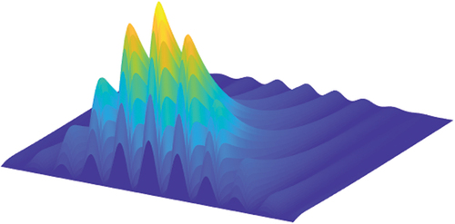
Figure 1. Hatched areas represent the ranges in wavevector (${\text{k}}_{\text{exc}}$) and frequency (${\omega }_{\text{exc}}$) typically accessible by optical transient grating (TG) and by the most common spectroscopic approaches used to study collective dynamics in condensed matter: Brilluoin and Raman light scattering (BLS and RLS), inelastic UV (IUVS), X-ray (IXS) and neutron scattering (INS). Black, red and blue lines sketch, respectively, typical dispersion curves for phonon frequency, heat transport time and magnonic oscillations. Magenta/orange horizontal lines sketch the typical upper/lower bounds for molecular vibrational frequencies; in many cases structural relaxation times also fall in this range.

Thermal and elastic properties are not the only intertwined aspects of condensed matter that pose open questions at the nanoscale. Another hot scientific topic regards the understanding of the coupling of magnetic spin to electron and lattice degrees of freedom observed in magnetically ordered metals, where light can induce ultrafast demagnetization within 100 fs [25]. After more than 25 years from its discovery a crucial question has remained elusive: how the spin angular momentum is dissipated among electronic and lattice excitations [26,27], and novel theoretical frameworks have been developed [28–30] without providing a general consensus on the underlying microscopic processes. More in general, the complexity of this spin-electron-lattice interaction determines material properties such as magnetic anisotropy or magnetostriction, which dictate the capability of controlling magnetic domain switching with light or manipulating magnetization with external fields [31–33]. The characteristic timescales for these dynamic magnetic processes, which are fundamental for technological applications like magnetic storage and spintronics, are in the ps timescale and beyond [25,34,35] and may even become comparable to the ultrafast electronic response via the optical inter-site spin transfer process [36,37]. Direct experimental access to macroscopic magnetic properties, for example the total magnetization, is granted by well-established methods. However, in many cases theories connecting macroscopic and microscopic information cannot explain the behaviour observed at the nanoscale and at ultrafast timescales. Beside ultrafast timescales, magnetic dynamics happening in the picosecond and longer timescales are also strongly affected by long- and short-range magnetic interactions, such as spin orbit coupling, dipolar, exchange and Dzyaloshinskii – Moriya interactions. Their interplay during the recovery of the magnetic order after an optical stimulus is the key aspect for the formation of complex spin textures like chiral domain walls, skyrmions, merons or bobbers [38], whose early stage formation dynamics is still under scrutiny [39–41]. Controlling this non-trivial real-space spin topology is expected to become extremely relevant in the near future for spintronics, which promises lower energy consumption and faster access times. In this context, experimental techniques used to probe ultrafast nanoscale dynamics in magnetic systems, including ultrafast optical spectroscopy, time-resolved X-ray diffraction and time-resolved scanning probe microscopy [42,43], can provide invaluable information to the quest of rationalising nanoscale magnetism.

The study and understanding of collective dynamics at the nanoscale and fs/ps timescale is thus the key to fill this knowledge gap, which nowadays is not only relevant for an academic scientific interest but has also critical implications for technological advances that are already playing a key role in our lifestyle. For instance, the knowledge of $D_T$ at the nanoscale is crucial to determine the rate at which the heat moves away from the region of a microchip where the computation is performed, thus defining the maximum computation rate to avoid device failure due to temperature build-up. In theory, the timescale for heat to flow over a few nm distance in a modern chip may enable computational clock frequencies as large as THz. However, while thermal transport models can be extended to the nanoscale by assuming size-dependent parameters, as $D_T$, the lack of a generally accepted and predictive theory for nanoscale heat transport makes the experimental approach essential, both for driving theory development and for phenomenologically designing efficient nano and quantum devices. Similarly, the functionalization of thin films through impurities or nanostructuration is one of the challenges of modern technology [44], with applications, among others, in energy harvesting, catalysis, thermal barrier coatings and phonon-engineered materials with extreme thermal properties. However, the impurities and nanostructures introduced to tailor the functionalities of the films are often detrimental for their elastic properties, up to device failure, an effect that is increasingly larger for thinner films [24]. The determination of thermoelastic properties of ultra-thin films and other layered structures requires space-time resolution in the nm-fs range. Access to this length- and time-scale range will also permit, e.g. to understand the limit of magnetic phenomena related to all optical switching in different classes of materials (30, 31), such as the quite astonishing phenomenology of the magnetization reversal in ferrimagnets that bases on the precession on different pathways of the rare-earth and transition metal ferromagnetic structures [45–47] and where magnetic reordering is achieved after a single optical excitation. In ferromagnetic structures, instead, circularly-polarised multi-pulse exposure is needed to reverse the spin direction, pointing towards a crucial role played by heat dissipation mechanisms after optical excitation [48,49]. Understanding and controlling these processes at the nanoscale will allow to engineer high speed spintronic devices with deterministic properties.

The experimental access to the nm-fs region presents technical difficulties as will be discussed in the next section. To overcome these technical hurdles we recently exploited the bright and ultrafast extreme ultraviolet (EUV) pulses generated by free electron lasers (FELs) to extend the transient grating (TG) method, a four wave mixing technique (FWM) [50,51], towards nanoscale wavelengths. In this review we will present the results obtained in the past few years and discuss the promising perspectives of EUV TG. Section 2 contains an overview of the state of the art in the investigation of ultrafast nanoscale material properties. Section 3 describes advantages and limitations of the TG approach and its extension to the EUV and X-ray regimes. Section 4 reports on some exemplary results with the intention to illustrate the potential of the technique. The current pioneering instruments and their prospective evolution are described in Section 5. Finally, Section 6 discusses the evolution of EUV TG and FWM beyond the proof of principle, both from a basic science and from a technology validation perspective.

2 Experimental methods for the investigation of collective dynamics

The experimental investigation of thermal, magnetic and elastic dynamics dates back more than a century, starting from methods based on calorimeters, magnetometers, mechanical spectrometers, acoustic transducers and photothermal cells [52–55]. These typically probe timescales in the second to μs range, i.e. downward out of range with respect to the time-space plane shown in Figure 1, even though the ns regime was made accessible for example by pulsed magnetic and electric fields generated by fast discharges [56,57] or by ultrasonic transducers [58]. Later on, the invention of the laser enhanced the capabilities of studying thermal properties by a number of phothermal methods, e.g. thermal lensing, photoacoustics spectroscopy and imaging [59–69].

2.1 Spectroscopic approach: dynamics of spontaneous fluctuations

After the laser invention a number of scattering spectroscopies was developed to cover large portions of the ($k_{exc},{\omega }_{exc}$)-plane shown in Figure 1, where $k_{exc}=\left|k_{exc}\right|$ and ${\omega }_{exc}$ are, respectively, the wavevector’s modulus and frequency of the excitations. This is the case of Brillouin light scattering (BLS) spectroscopy, which provided access to lattice vibrations at hypersonic frequencies [70,71] well above the GHz regime, as well as magnons and other magnetic excitations [72–74], while Raman light scattering (RLS) [75], THz/mid-IR absorption and imaging probed THz excitations of both vibrational and magnetic nature [76]. These laser-based techniques are sensitive to either the spontaneous fluctuations of the experimental observable, i.e. the refractive index, or the dissipation of light intensity into the specimen. In both cases the encoded information refers to the thermal population of collective excitations associated with a given $k_{exc}$. Absorption techniques are restricted to $k_{exc}=0$, while scattering methods can probe finite values of $k_{exc}$. However, the accessible range in $k_{exc}$ has an upper limit given by the laser wavelength ($\lambda \sim$ 1 μm) and the refractive index of the sample (n): $k_{exc}=4\pi n/\lambda$. Even if instruments capable of working with UV wavelengths ($\lambda \sim$ 200–300 nm) were devised [77,78], such a boundary prevents the extension of laser-based spectroscopies to nm length-scales.

A suitable spectroscopic probe for collective excitations at large $k_{exc}$ in condensed matter was available since the late 50s with the development of inelastic thermal neutron scattering (INS) methods [79], which, paraphrasing the press release for the Nobel prize awarded in 1989 to Shull and Brockhouse [80], helped answer the question of where atoms ‘are’ and what atoms ‘do’. In fact, the wavefunctions of thermal neutrons have both the right (De Broglie) wavelength and frequency ($\lambda \sim 10-0.01$nm and $\omega \sim 0.1-10$THz) to be sensitive to interatomic distances and lattice dynamics. This enables them to probe the full phonon dispersion relations [81], and even to reach higher order Brillouin zones. Moreover, the 1/2 spin due to their fermionic nature allows interaction with the elementary constituents of magnetic materials, therefore permitting sensitivity to magnetic structures and collective magnetic excitations. This enabled the experimental determination of magnons [82]. As in any scattering technique, the accessible range in $\left(k_{exc},{\omega }_{exc}\right)$ is limited by energy and momentum conservation. In the specific case of neutrons, which are massive particles, the relation between mass, momentum and kinetic energy inherently precludes to simultaneously have De Broglie wavelengths of about one nm and frequencies exceeding a THz, thus preventing the possibility to probe ps dynamics in the aforementioned 10s of nm scale of interest (see Figure 1).

In the frequency range of interest for collective lattice excitations, i.e. not exceeding the 100s of THz regime, these kinematic constraints are overcome by high resolution inelastic hard X-ray scattering (IXS). The detection of lattice excitations at X-ray wavelengths (≈0.1 nm) via IXS requires the spectroscopic determination of relative photon energy shifts that are typically a fraction of the ratio between the speed of sound and the speed of light, i.e. 10⁻⁵ − 10⁻⁷. IXS was developed in the late 90s with the availability of synchrotron light sources for users and the advent of hard X-ray spectrometers with up to 10⁸ resolving power [83,84]; indeed, the required high resolution inherently reduces the signal intensity and only X-ray sources with very high average flux can mitigate this issue. IXS also overcomes other relevant hurdles of INS, as, for example, the low flux and large spot size at sample, as well as safety aspects. Though X-rays do not directly interact with spins significantly, since there are no spin-dependent terms in the dipole operator and the magnetic field of X-ray oscillates too fast to be ‘seen’ by electrons, in certain conditions the spin-orbit coupling enables observable interactions of X-rays with the spin system [85]. Despite some attempts to further improve the performances of spectrometers [86,87], the frequency range below 1 THz is hardly accessible, therefore impeding obtaining dynamic information on timescales longer than a few ps. Again, this situation practically prevents studying collective excitations at the 10s of nm length scale (see Figure 1), since the dynamics of those excitations span longer timescales.

Analogously to BLS and RLS, INS and IXS probe the spectrum of the fluctuations of the dynamic observables, which naturally arise from a thermal population of collective excitations. To obtain significant signals, all these methods need a proper scattering volume, which is typically limited by radiation absorption lengths. This imposes important constraints in the use of laser-based BLS and RLS from samples opaque to optical radiation, e.g. metals. Conversely, hard X-rays and neutrons can penetrate all types of specimens, although the low inelastic scattering cross section practically forbids the use of thin samples and the extremely low reflectivity makes it hard to achieve surface sensitivity [88]. In general, very thin samples (<1 µm) are hardly viable also for BLS and RLS. Samples used in IXS, INS and visible scattering methods are often mm thick or even longer.

The intermediate nm-ps range highlighted in Figure 1 could be in principle accessible by inelastic scattering of EUV radiation, at least for what concerns the thermoelastic response. However, there are two main aspects that hinder this development. A technological one that consists in the lack of EUV spectrometers with sufficient resolving power (>10⁶) and photon throughput [89,90], and a fundamental one related to the fact that all materials show a very short EUV absorption length (typically <1 µm), inherently reducing the scattering volume and hence the inelastic scattering signal. The latter issue can be radically addressed by using photon sources with average flux larger than synchrotrons, such as high repetition rate FELs, which, indeed, are being profitably employed for EUV and soft X-ray spectroscopy [89,91–93].

2.2 Pump-probe approach: stimulated dynamics

An alternative to the spectroscopic detection of the fluctuations spectra of dynamical variables is to measure collective modes in the time-domain through the use of pump-probe techniques, where the excitations in the sample are created by a first pulse (pump) and are probed by a second pulse (probe) impinging on the sample after a given time interval ($\mathrm{\Delta }t$). This experimental concept has been largely developed based on pulsed lasers, where two time-delayed optical pulses can be straightforwardly produced. Optical setups even allow to easily generate two pulses with different wavelengths or polarisations. On one hand this helps to distinguish pump and probe pulses and decrease signal to noise (S/N) at the detector, on the other it can be exploited to selectively excite one process and probe a different one.

The pump-probe approach is naturally suited to detect the sample response on long timescale ranges, since values of $\mathrm{\Delta }t$ as large as ns correspond to optical delay lengths of about a metre, easily realisable in any laboratory. This already permits to overcome the main technical showstopper for developing EUV methods able to probe collective lattice dynamics in the frequency domain: the limited resolving power of EUV spectrometers. 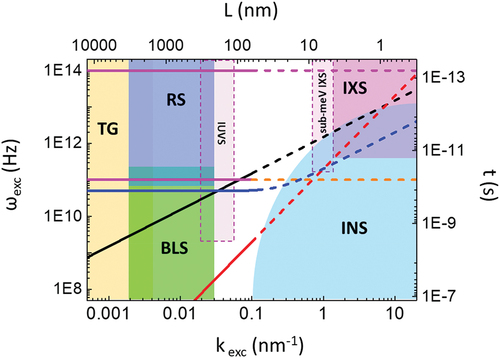Furthermore, if the time duration of the pump pulse ($\mathrm{\Delta }{t}_{pump}$) is shorter than the dynamics of interest, then all sample excitations generated by the pump can be considered as coherent in time, i.e. they can be assumed to be generated at the same instant, and the signal amplitudes add up in phase, with a large increase in the efficiency of the experiment. To illustrate this concept, we sketch in Figure 2 the time-dependent amplitude of a dynamic variable having the shape of a sinusoidal modulation with period $t_{mod}$. This is representative of a density modulation due to an acoustic phonon with a given period $t_{mod}=t_{ph}=2\pi /{\omega }_{ph}$ and the phonon decay is neglected. Assuming that all the photons in the pump pulse have a certain probability to generate such a phonon, if $\mathrm{\Delta }t\ll t_{ph}$ all phonons are generated in a narrow time window and the amplitudes of the density modulation associated to each individual phonon add up coherently (i.e. in phase); Figure 2a). If the probe pulse is sensitive to density changes, e.g. via a density dependence of the refractive index, the experimental signal results to be larger because of the coherent addition of the amplitudes of the individual excitations. This is no longer true if $\mathrm{\Delta }{t}_{pump}\approx t_{ph}$ or $\mathrm{\Delta }{t}_{pump}>t_{ph}$, since in these conditions the modulation is washed out; see Figure 2b-c). Ultrafast optical lasers can easily meet the conditions for impulsive excitation of lattice vibrations in the whole frequency range of interest and also provide a suitable probe for these dynamics, i.e. with a time duration ($\sim$ 10s of fs) shorter than the relevant timescale of the sample response. In fact, optical pulses as short as a few 10s of fs are routinely available, thus enabling to excite and probe phonons with angular frequency as large as some 100s of THz, basically covering a range up to that exploitable by IXS and INS. Such capability was exploited in picosecond ultrasonic [69,94], which represented a manifold of advances in fundamental and applied research, ranging from, e.g. nonlinear phononics [95,96] and elasticity in extreme conditions [97] to nanotechnology [98–101], imaging and biology [102,103].

Figure 2. Time-dependent amplitude of a dynamic variable impulsively excited at $\mathrm{\Delta }\text{t}=0$ by a pump pulse (blue trapezoid), for illustration purposes we assumed a sinusoidal time dependence. The red full lines are the amplitudes of single excitations, all of them generated within the time duration of the pump ($\mathrm{\Delta }{\text{t}}_{\text{pump}}$), while the black dotted one is their average. Panels a), b) and c) depict, respectively, the conditions $\mathrm{\Delta }{\text{t}}_{\text{pump}}\ll {\text{t}}_{\text{mod}}$, $\mathrm{\Delta }{\text{t}}_{\text{pump}}<{\text{t}}_{\text{mod}}$ and $\mathrm{\Delta }{\text{t}}_{\text{pump}}\approx {\text{t}}_{\text{mod}}$, where ${\text{t}}_{\text{mod}}$ is the period of the sinusoidal modulation.

Analogously, pump-probe approaches provided relevant advances for the study of the thermal response, e.g. via thermoreflectance and thermal imaging methods [32,104,105], as well as allowed studying the magnetic response in a previously unexplored range. This permitted, for instance, to discover the still debated process of ultrafast demagnetization [25], to achieve heat assisted magnetic recording [106] or to probe coherent magnons [107,108] and their coupling to vibrational excitations [109]. Despite not being constrained in the time-scale axis, the generation of short wavelength excitations with an optical fs pulse requires the use of artificial nanoscale structures, which are realised on the sample of interest, as thin metal films, wedges, superlattices, nanobars or nanodots [24,69,110–116]. In this way sample excitations with a few nm wavelength can be generated [110], while broadband optical probes and high refractive index substrates can be used to detect dynamics in a large $\left(k_{exc},{\omega }_{exc}\right)$-range [117]. However, the need of properly shaping or modifying the sample is an inherent complication that in some cases limits the use of these approaches. When nanostructures are not used, optical excitation of collective modes is limited in the wavelength axis by the laser wavelength, as discussed above for the scattering methods. An alternative to coherently stimulate collective excitation without the aid of transducers or other nanostructures is to employ an optical TG [118–121], where the excitation wavevector is determined by the interference pattern of two crossed light pulses. The capability of TG to flexibly control the wavevector was initially used for laser ultrasonics [122], as well as for studying relaxation dynamics [123] and transport processes [124]. However, the TG approach can be in general applied to study any kind of phenomena resulting in a modification of the refractive index. This flexibility has permitted to investigate many other different processes, such as carrier and spin dynamics [125–128], polaritons [129], molecular dynamics [130], heat diffusion [5,131] and heat waves [132], charge density waves [133] and laser-plasma interactions [134]. Furthermore, the very high S/N of this method permitted it to be applied in in a number of samples, like surfaces [135,136], proteins in solution [137,138], nanostructures [138], vapours [139] and molecular beams [140], demonstrating the capability to span time delay ranges from a few fs [141] to seconds [142], while the generalized concept of TG was exploited in many other types of FWM experiments [143], such as photon echo and coherent Raman scattering. Simple and robust setups for optical TG permit to reliably exploit few fs pulses [144,145], as well as to use the TG approach for ultrafast photo-diagnostics [146] or for metrology in industrial environments [147,148].

2.3 Short-wavelength pulses

The advent of high-harmonic generation (HHG) sources has provided ultrafast (down to sub-fs) pulses of EUV radiation that can be employed as a sensitive probe in pump-probe experiments, including TG. Already from the first pioneering optical TG experiments with EUV probes [149], the shorter probe wavelength (${\lambda }_{probe}$) enhanced the sensitivity to coherent surface displacements induced by the propagation of surface acoustic waves (SAWs) launched by the optical TG. To overcome the inherent limit concerning the short wavelengths excitable by optical TG, picosecond ultrasonics in combination with different kinds of sample nanostructuration and EUV probing are currently employed [22–24,116,150,150]. These are excellent methods to detect various types of thermoelastic processes, such as nanoscale thermal transport and elasticity, and permitted to study the transition from diffusive to ballistic regime of heat transport at room temperatures [115], to postulate new regimes occurring at the nanoscale [24], as well as to characterise the effects of impurities and thickness on the elastic moduli in ultra-thin films (down to a few nm), multilayers and metalattices [23,24,114,150]. These investigations are the key to devise, e.g. new materials with extreme thermal properties and to understand the roles of interfaces and scattering at the nanoscale, information that can be used for ‘phonon engineering’ matter at the nanoscale [115]. The high energy of EUV photons ($E_{EUV}$) also enabled the exploitation of core resonances, thus making the probe process element-specific. This feature was also employed in combination with optical TG excitations, to investigate the generation of four-wave-mixing signals on a few fs timescales in an archetypal sample, i.e. atomic He [145,151], and to study the insulator to metal transition in crystalline VO₂ [152]. EUV spectroscopy with HHG is used in many other types of pump-probe techniques, ranging from atomic and molecular physics to condensed matter dynamics. In particular, the improvements of HHG sources in last decade [153], which include the capability to generate EUV pulses at the M-edges of ferromagnetic elements, permitted, e.g. to explore intersite spin transport phenomena in magnetic alloys [36,37], the differences in spin wave injection across ferromagnetically/antiferromagnetically coupled heterojunctions [35] and real space time-resolved imaging [154].

Probe pulses in a much broader photon energy range (up to hard X-rays) and with tunability largely surpassing the one achievable by HHG sources, in both photon wavelength and polarisation, are available at synchrotron sources. Though limited to pulse durations of 10s of ps or longer, these can potentially provide spatial resolution at the atomic scale. Indeed, they were successfully employed to detect the effects on the atomic motion of the thermoelastic excitation induced by optical TGs, since these dynamics take place on substantially longer timescales [155]. X-ray synchrotron pulses are used in many other pump-probe experiments, combining optical pump with the full range of diffraction, spectroscopy and dichroic methods developed at synchrotrons and used as a probe. For example, as discussed above, optical pulses can trigger coherent phonons and lead to the nonthermal switching between SET and RESET states in phase change materials; time-resolved x-ray diffraction has been used to investigate this and other kinds of structural dynamics [156–159]. Tuning of thermal properties in technological materials through phonon engineering is achievable by characterising the ultrafast evolution of selected Bragg peaks from sample materials exposed to infrared femtosecond pulses [101,160] and light-driven surface structure rearrangement dynamics in dichalcogenides MX₂ (transition metal M and chalcogen X) have been monitored through X-ray photoemission spectroscopy [161,162]. Those approaches also allowed access to slower magnetic dynamics, for example domain wall motion [163] stimulated by strong pulses of current, SAW induced manipulation of the magnetic state in coupled nanostructures at the ps scale, as a consequence of the effective variation in the magnetic free energy [164,165], or gyrotropic motion of the large skyrmion bubbles [166]. All these applications need sub-ns temporal resolution [85,167–169] and sub-30 nm spatial resolution [170–172].

We finally mention that the time structure of synchrotron radiation sources was used also without the aid of optical pumps to detect dynamical processes: this is the case of magnetization reversal dynamics at surfaces and interfaces, determined by soft X-ray photoemission through the synchronised detection of spin-polarised photo-emitted electrons [173]. Synchrotron sources are also characterised by an extremely high repetition rate, up to the GHz regime, that ensures an average brilliance comparable with many optical lasers. Though schemes for enabling synchrotron pulses in the few ps range (and potentially beyond) are possible and some of them already implemented [174,175], their pulse duration is still insufficient to be used in ultrafast pump-probe schemes typical of optical table-top experiments. Similarly, HHG sources do not provide sufficient flux. This combination is today available only at X-ray FELs and permitted to implement new types of ultrafast X-ray experiments, which in some cases can be used to probe phonons at X-rays wavevectors in the time-domain [176–178]. Ultrafast X-ray pulses from FELs have been used in various other ways to probe dynamical processes in condensed matter. For instance ultrafast X-ray magnetic diffraction and imaging were used to study ultrafast demagnetization at the nanoscale with element selectivity, not available with optical methods [179–184] opening the pathway to controlling nonlinear dynamics of spin systems [185–187] via intense EUV pulses.

We have so far presented the use of EUV and X-ray pulses as a probe for condensed matter dynamics. FEL pulses, that are orders of magnitude more intense [188] than those of synchrotrons and HHG sources, can not only stimulate dynamics by bringing the sample in a moderately out of equilibrium state [189–191], but in many cases can provide sufficient pulse brilliance (i.e. enough photons in a single pulse) to drive the sample through phase transitions or irreversibly bring condensed matter into extreme states [192–195]. FEL sources are thus the ideal platform to carry out ultrafast EUV TG experiments at sub-100 nm length-scale, for which femtosecond EUV pulses are needed both for pump and probing in an FEL-pump/FEL-probe approach. This situation is quite uncommon in the panorama of FEL-based methods and has been implemented at the FERMI FEL in a dedicated instrument that is routinely used by the scientific community [118,196,197].

2.3.1 FEL sources

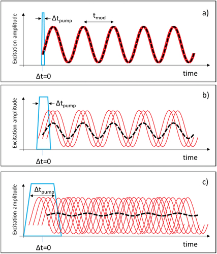
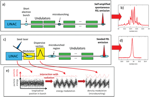
EUV and X-ray FELs are large scale photon sources (100s m to a few km long), typically consisting of a photoinjector gun that generates short electron bunches, a linear accelerator (LINAC) that accelerates the bunches up to a given (ultrarelativistic) electron energy and a radiator section [198,199]; see Figure 3a). The latter is commonly made of periodic magnetic structures (undulators), which impose periodic transverse accelerations with respect to the propagation direction of the bunch. The electrons thus wiggle while they propagate along the radiator section and emit EUV/X-ray light at each wiggle, at a wavelength that depends on the electron energy, and periodicity and strength of the magnetic structure, while the number of emitted photons is proportional to number of electrons in the bunch. However, if the radiator section is sufficiently long, a feedback mechanism is spontaneously established and results in a longitudinal density modulation of the electron bunch, with a periodicity equal to the wavelength of the emitted light. The electric field amplitudes of the light emitted by the electrons at each wiggle thus add in phase and the total amount of radiated photons is $\propto N_e^2$, where $N_e\approx$ 10⁸ is the number of electrons in the bunch that can be correlated in phase, instead of being $\propto N_e$, as it would be in a conventional undulator. This process is known as self-amplified spontaneous emission (SASE), resulting in FEL light characterised by a number of longitudinal modes with random phases, which ultimately originate from the density fluctuations (i.e. the ‘noise’) in the electron bunch [200]. This results in a ‘spiky’ spectrum (see Figure 3b) and time structure, within a temporal envelope as short as a few fs. These structures change from shot to shot, since they arise from stochastic fluctuations. Alternatively, FEL light can be generated by external seeding (see Figure 3c), e.g. through the so-called high gain harmonic generation process [201], resulting in a single mode FEL spectrum (see Figure 3d). In a seeding scheme, a laser pulse with wavelength ${\lambda }_{seed}$ interacts with the electron beam in a short undulator section, called modulator and placed at the output of the LINAC, imposing an energy modulation on the electron beam. This energy modulation is converted into a density modulation through a dispersive section, consisting of a magnetic chicane where electrons with lower energy follow longer trajectories and are thus delayed with respect to higher energy electrons (see Figure 3 e). The electron beam at the output of the chicane has a sawtooth-like density profile with a spatial periodicity equal to ${\lambda }_{seed}$ and the Fourier spectrum of the longitudinal electron density contains a sizable number of high harmonics. The undulators can be tuned to amplify only one of these and the output is a nearly Fourier transform limited FEL pulse with wavelength ${\lambda }_{FEL}={\lambda }_{seed}/N$, where N is an integer number (see Figure 3d). Furthermore, the FEL emission inherits properties such as time duration and temporal coherence from the seed laser. The drawbacks of the seeding scheme are: i) a lower pulse energy, but still in the 10s to 100s µJ range at the FEL output [202]; ii) a longer pulse duration, which is related to the time duration of the seed and typically limited to the 10s of fs scale, though in some conditions the pulse duration can be substantially shortened [203]; iii) most importantly, the shorter FEL wavelength that can be reached (through a double cascade scheme [204]) is limited to the $\approx$ 4 nm range because of the decreasing amplitude of higher harmonics of the sawtooth-like density modulations, though FEL harmonics with substantial intensity were observed down to $\approx$ 1.5 nm [205]. Other seeding schemes are currently under investigation to extend the output range [206]. The FERMI FEL (Trieste, Italy) is nowadays the only short wavelength FEL based on this scheme [207]. The FLASH FEL (Hamburg, Germany) will soon open a new FEL line based on the external seeding scheme [208,209].

Figure 3. a) sketch of the SASE FEL generation process: the microbunching develops throughout the undulator section and involves all the (short) electron bunch. The spectrum of the resulting (multi-mode) output FEL pulse is illustrated in panel b). Panel c) schematizes the seeding scheme for FEL generation, a considerable microbunching is already present at the input of the undulator section and involves only the region where the interaction with the seed laser pulse has occurred. The spectrum of the output radiation consists in a single mode, as shown in panel d). The process of inducing an energy modulation (via the interaction with the seed laser) and to convert it into a density modulation (through a dispersive magnetic section) is illustrated in Panel e), where the energy of the electrons in the bunch as a function of the longitudinal coordinate is shown at the output of the LINAC (left plot), of the modulator (middle plot) and of the dispersive section (right plot); see also red arrows.

The FERMI FEL has two accelerator lines: FEL1 and FEL2, covering respectively the 18–100 nm and 4–18 nm range; these two sources cannot be operated in the same run. While FEL1 works with the seeding scheme described above [201], FEL2 is a two stage FEL working in cascade [204]. The first stage operates as described above and its emission is used as seeding wavelength for the second stage. The two stages are separated by a delay line for the electrons that synchronises the first stage emission with a fresh part of the bunch for the second stage amplification. Ultimately, FEL2 emission has a wavelength ${\lambda }_{FEL}={\lambda }_{seed}/MN$ where N is the first stage harmonic number and M the second stage one. This cascade configuration makes FEL2 an ideal source for multicolour schemes, since first and second stage emissions can be used simultaneously and are intrinsically time-overlapped. Multicolor schemes are possible also with FEL1 at the expenses of the overall emission intensity, using the so-called split undulator configuration where a portion of the undulators is tuned at harmonic $N_1$ and the other at $N_2$ [210], thus resulting in a dual wavelength FEL output (${\lambda }_{FEL,1}={\lambda }_{seed}/N_1$ and ${\lambda }_{FEL,2}={\lambda }_{seed}/N_2$). Three or more outputs as well as phase control are also possible [211–213].

3 The EUV TG method

The TG method relies on a nonlinear optical interaction. At the core of NL optics is the polarisation (P) response of a material to an intense electromagnetic field of amplitude E [50]: Equation 1(1) $P={\chi }^{\left(1\right)}E+{\chi }^{\left(2\right)}EE+{\chi }^{(3)}EEE+\dots$(1)

(1) $P={\chi }^{\left(1\right)}E+{\chi }^{\left(2\right)}EE+{\chi }^{(3)}EEE+\dots$(1)

where ${\chi }^{\left(1\right)}$ is a (N + 1)-rank tensor referred to as N^th-order susceptibility; ${\chi }^{\left(2N\right)}$ is zero in media with inversion symmetry while ${\chi }^{\left(2N+1\right)}$ has non-zero elements for any sample symmetry. ${\chi }^{\left(1\right)}$E represents the 1^st order polarisation, which determines all linear light-matter interactions. The polarisation term associated with the 3^rd order susceptibility, the first non-zero nonlinear order in any material, gives rise to FWM processes. A generic FWM experiment is depicted in the panel a) of Figure 4. Here the interaction on the sample with three beams, each with its wavevector $k_i$, frequency ${\omega }_i$, relative arrival time $\mathrm{\Delta }{t}_{ij}$ and polarisation unit vector $\widehat{p_i}$, with i,j = 1–3, generates the fourth beam that is the FWM signal, having its own $k_4,{\omega }_4,\mathrm{\Delta }{t}_{i4}$ and $\widehat{p_4}$. FWM schemes are very diverse, depending on the combination of $k_i$, ${\omega }_i$, $t_i$ and $\widehat{p_i}$, giving rise to several methods, e.g. 3^rd harmonic generation, coherent anti-stokes Raman scattering, photon echo, multidimensional spectroscopies, TG, etc.

Figure 4. a) sketch of a FWM experiment, red, green and blue pulses are the three beams impinging into the sample, while the magenta one is the signal beam; $\mathrm{\Delta }{\text{t}}_{\text{i},\text{j},3}$ are the delays between these four pulses. b) Scheme of a TG experiment with the relevant quantities (see text), the reference frame is shown in the top-right corner.

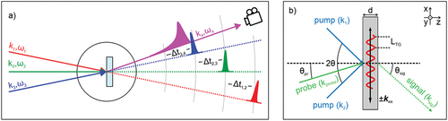
In the specific case of TG, two pulses of equal wavelength ${\lambda }_{pump}$ are overlapped in space and time at the sample surface with a crossing angle $2\theta$; this implies that the wavevectors of these two pulses ($k_1$ and $k_2$) have equal magnitude but different directions. Assuming that a planar sample with a given thickness d is oriented with the surface normal parallel to the bisector of the pump beams (see Figure 4b), their sinusoidal interference pattern results in a TG excitation with periodicity $L_{TG}$ that depends only on ${\lambda }_{pump}$ and $2\theta$ as: Equation 2(2) $L_{TG}={\lambda }_{pump}/\left[2sin\left(\theta \right)\right].$(2)

(2) $L_{TG}={\lambda }_{pump}/\left[2sin\left(\theta \right)\right].$(2)

The wavevector of the TG excitation, $k_{exc}=\pm k_{TG}$ (with $k_{TG}=2\pi /L_{TG}$) lies in the plane defined by the two interfering (pump) beams and is parallel to the sample surface, corresponding to the spatial coordinate x (see Figure 4b). The spatial modulation of light intensity imposed by the TG may turn (via light-matter interactions) in a transient sinusoidal modulation of the complex refractive index, i.e [119–121,214]: Equation 3(3) $n\left({\lambda }_{probe};x,\mathrm{\Delta }t\right)=n\left({\lambda }_{probe}\right)+\mathrm{\Delta }n\left({\lambda }_{probe};\mathrm{\Delta }t\right)cos(2\pi x/L_{TG}{)}_{},$(3)

(3) $n\left({\lambda }_{probe};x,\mathrm{\Delta }t\right)=n\left({\lambda }_{probe}\right)+\mathrm{\Delta }n\left({\lambda }_{probe};\mathrm{\Delta }t\right)cos(2\pi x/L_{TG}{)}_{},$(3)

where we assumed that at any spatial location the refractive index variation ($\mathrm{\Delta }n$) is linearly proportional to the intensity of the interference pattern and the excitation is uniform along the sample depth (spatial coordinate z; see Figure 4 b). This patterned excitation can thus effectively act as a transient diffraction grating for a third variable-delayed (probe) pulse of wavelength ${\lambda }_{probe}$ and wavevector $k_{probe}$, provided that $\mathrm{\Delta }n\left({\lambda }_{probe},\mathrm{\Delta }t\right)\ne 0$, giving rise to a fourth pulse: the diffracted (signal) beam. The signal beam normally has the same wavelength as the probe while the propagation direction of the first diffraction order in the x-z plane is determined by the diffraction angle ${\theta }_{sig}$, given by: Equation 4(4) $L_{TG}\left[sin\left({\theta }_{sig}\right)+sin\left({\theta }_{probe}\right)\right]={\lambda }_{probe},$(4)

(4) $L_{TG}\left[sin\left({\theta }_{sig}\right)+sin\left({\theta }_{probe}\right)\right]={\lambda }_{probe},$(4)

where ${\theta }_{probe}$ is the probe incidence angle. Higher diffraction orders may be observable in thin samples or for non-sinusoidal excitation patterns, achievable, e.g. when the dependence of $\mathrm{\Delta }n$ on the intensity of the interference pattern is not linear [215]. The signal beam parameters (intensity, polarisation, etc.) as a function of $\mathrm{\Delta }t$ encode the dynamics of the photoexcited processes that are characterised by the wavevector $k_{exc}$.

The main limitation of the TG technique in the optical regime is readily evident Equation 1(1) $P={\chi }^{\left(1\right)}E+{\chi }^{\left(2\right)}EE+{\chi }^{(3)}EEE+\dots$(1) , which defines a lower limit for $L_{TG}>{\lambda }_{pump}/2$, and thus a maximum possible value for $k_{exc}$, which in case of optical wavelengths (${\lambda }_{pump}\approx$ μm) locates at $k_{exc}\approx$ 0.01 nm⁻¹ (see also Figure 1). Excitation pulses at EUV wavelength (${\lambda }_{pump}\approx$ 10–100 nm) can in principle overcome this limitation, upscaling $k_{exc}$ by 1–2 orders of magnitudes. Clearly, an EUV pulse is also needed for probing EUV TGs at short values of $L_{TG}$ (unless another type of short wavelength probe is used, e.g. electron bunches [216]). In fact, similarly to Equation 2(2) $L_{TG}={\lambda }_{pump}/\left[2sin\left(\theta \right)\right].$(2) for the pump, Equation 4(4) $L_{TG}\left[sin\left({\theta }_{sig}\right)+sin\left({\theta }_{probe}\right)\right]={\lambda }_{probe},$(4) defines an upper limit for the probe wavelength at ${\lambda }_{probe}<2L_{TG}$.

3.1 Diffraction efficiency (forward diffraction)

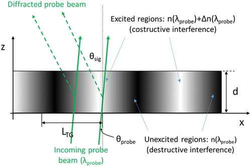
The experimental observable in a TG experiment is the time-dependent diffraction efficiency ${\eta }_F\left(\mathrm{\Delta }t\right)=I_{sig}\left(\mathrm{\Delta }t\right)/I_{probe}$, where $I_{sig}\left(\mathrm{\Delta }t\right)$ and$I_{probe}$ are, respectively, the (time-dependent) signal intensity and the probe incident intensity. In a forward diffraction geometry like the one sketched in Figure 4b), the excited sample is crossed by the probe beam and diffraction is caused by the phase and absorption differences accumulated by the different portions of the probe beam that propagates through sample locations with different values of $n\left({\lambda }_{probe};x,\mathrm{\Delta }t\right)$, as illustrated in Figure 5. This figure illustrates a uniform excitation along z, in agreement with Equation 3(3) $n\left({\lambda }_{probe};x,\mathrm{\Delta }t\right)=n\left({\lambda }_{probe}\right)+\mathrm{\Delta }n\left({\lambda }_{probe};\mathrm{\Delta }t\right)cos(2\pi x/L_{TG}{)}_{},$(3) , a condition that can be commonly meet in optical TG but is unlikely for EUV TG. Indeed, in realistic cases the EUV light is strongly absorbed by any material, with absorption lengths $L_{abs}$ typically comparable with the values of $L_{TG}$ reachable by the EUV TG excitation itself (10s-100s nm). In these conditions the EUV TG excitation is no longer unidimensional and the refractive index variation shows a dependence on z; Equation 3(3) $n\left({\lambda }_{probe};x,\mathrm{\Delta }t\right)=n\left({\lambda }_{probe}\right)+\mathrm{\Delta }n\left({\lambda }_{probe};\mathrm{\Delta }t\right)cos(2\pi x/L_{TG}{)}_{},$(3) can hence be rewritten as: Equation 5(5) $\begin{array}{ll}n\left({\lambda }_{probe};x,z,\mathrm{\Delta }t\right)& =n\left({\lambda }_{probe}\right)+\mathrm{\Delta }n\left({\lambda }_{probe};\mathrm{\Delta }t\right)\\ & \times cos\left(2\pi x/L_{TG})exp(-z/L_{abs}\right)\end{array}$(5)

Figure 5. Diffraction of the probe from a sample of thickness d excited by a TG with spatial periodicity ${\text{L}}_{\text{TG}}$. Darker and lighter areas represent, respectively, the alternate unexcited and excited regions. Solid and dashed lines are the probe and signal beams, respectively.

(5) $\begin{array}{ll}n\left({\lambda }_{probe};x,z,\mathrm{\Delta }t\right)& =n\left({\lambda }_{probe}\right)+\mathrm{\Delta }n\left({\lambda }_{probe};\mathrm{\Delta }t\right)\\ & \times cos\left(2\pi x/L_{TG})exp(-z/L_{abs}\right)\end{array}$(5)

where $\mathrm{\Delta }n$ has to be regarded as the amplitude of the refractive index variation at the sample surface exposed to the FEL pump beams. Using Equation 5(5) $\begin{array}{ll}n\left({\lambda }_{probe};x,z,\mathrm{\Delta }t\right)& =n\left({\lambda }_{probe}\right)+\mathrm{\Delta }n\left({\lambda }_{probe};\mathrm{\Delta }t\right)\\ & \times cos\left(2\pi x/L_{TG})exp(-z/L_{abs}\right)\end{array}$(5) and further assuming a finite attenuation length for the probe beam, the TG response when absorption is not negligible can be derived, while the effect of finite spatial overlap between incidence pulses at a given crossing angle can be accounted for by assuming Gaussian beams with finite transverse dimensions and time duration. These important aspects are discussed in detail elsewhere [118]; in the following we briefly present the main points, which are rationalized in Equation 6(6) ${\eta }_F\left(\mathrm{\Delta }t\right)=\frac{I_{sig}}{I_{probe}}={\left|\mathrm{\Delta }n\left({\lambda }_{probe};\mathrm{\Delta }t\right)\right|}^{2}F\left({\lambda }_i,{\theta }_i,L_i,d\right)\xi \left({\sigma }_i,\mathrm{\Delta }{t}_{pump}\right),$(6) -Equation 8(8) $\xi \left({\sigma }_i,\mathrm{\Delta }{t}_{pump}\right)={\left(1+\frac{2{\sigma }_{probe}^2}{{\sigma }_{pump}^2}+\frac{2{\sigma }_{probe}^2}{L_{int}^2}\right)}^{-\frac{1}{2}}{\left(1+\frac{2{\sigma }_{probe}^2}{{\sigma }_{pump}^2}\right)}^{-\frac{1}{2}}.$(8) .

Within the aforementioned assumptions, ${\eta }_F$ is given by the product of three factors, as indicated in Equation 6(6) ${\eta }_F\left(\mathrm{\Delta }t\right)=\frac{I_{sig}}{I_{probe}}={\left|\mathrm{\Delta }n\left({\lambda }_{probe};\mathrm{\Delta }t\right)\right|}^{2}F\left({\lambda }_i,{\theta }_i,L_i,d\right)\xi \left({\sigma }_i,\mathrm{\Delta }{t}_{pump}\right),$(6) :

(6) ${\eta }_F\left(\mathrm{\Delta }t\right)=\frac{I_{sig}}{I_{probe}}={\left|\mathrm{\Delta }n\left({\lambda }_{probe};\mathrm{\Delta }t\right)\right|}^{2}F\left({\lambda }_i,{\theta }_i,L_i,d\right)\xi \left({\sigma }_i,\mathrm{\Delta }{t}_{pump}\right),$(6)

with

(7) $\begin{array}{ll}F\left({\lambda }_i,{\theta }_i,L_i,d\right)=& \frac{cos{\theta }_{sig}}{cos{\theta }_{probe}}{\left[\pi n\left({\lambda }_{probe}\right)d/{\lambda }_{probe}cos\left({\theta }_{probe}\right)\right]}^2\\ & \times \frac{e^{-\left(d/2L^{\ast }\right)}-2cos\left(\mathrm{\Delta }{K}_{z}d\right)e^{-\left(d/2L^{\ast }\right)}+1}{{\left(d/2L^{\ast }\right)}^2+{\left(\mathrm{\Delta }{K}_{z}d\right)}^2}{e}^{-d/L_{abs,probe}cos{\theta }_{sig}},\end{array}$(7)

where $$\begin{gathered} L^{\ast }=((L_{abs,pump}cos\left(\theta \right)/2{)}^{-1}+(L_{abs,probe}cos\left({\theta }_{probe}\right){)}^{-1}-{\left(L_{abs,probe} \\ cos\left({\theta }_{sig}\right){)}^{-1}\right)}^{-1} \end{gathered}$$, and Equation 8(8) $\xi \left({\sigma }_i,\mathrm{\Delta }{t}_{pump}\right)={\left(1+\frac{2{\sigma }_{probe}^2}{{\sigma }_{pump}^2}+\frac{2{\sigma }_{probe}^2}{L_{int}^2}\right)}^{-\frac{1}{2}}{\left(1+\frac{2{\sigma }_{probe}^2}{{\sigma }_{pump}^2}\right)}^{-\frac{1}{2}}.$(8)

(8) $\xi \left({\sigma }_i,\mathrm{\Delta }{t}_{pump}\right)={\left(1+\frac{2{\sigma }_{probe}^2}{{\sigma }_{pump}^2}+\frac{2{\sigma }_{probe}^2}{L_{int}^2}\right)}^{-\frac{1}{2}}{\left(1+\frac{2{\sigma }_{probe}^2}{{\sigma }_{pump}^2}\right)}^{-\frac{1}{2}}.$(8)

Here $\sigma$ indicates the beam size projected on the sample surface and $L_{int}=c\mathrm{\Delta }{t}_{pump}/tan\left(\theta \right)$, with c the speed of light, is the effective interaction region of the crossed excitation beams, assuming wavefronts orthogonal to $k_{pump1,pump2}$; see [118,217] and section 5 for further details. $\xi ({\sigma }_i,\mathrm{\Delta }{t}_p{)}_{}$takes into account the spatial overlap of the three beams and exclusively depends on the experimental scheme. In the optical regime this term typically approximates to unity and, thanks to the availability of diffractive split and recombination systems [144], the dependence on $\mathrm{\Delta }{t}_{pump}$ may drop. $\xi$ can become strongly relevant in the EUV regime due to practical experimental constraints, among them the wavefront tilt at the sample position due to the use of reflective optics for the split and recombination system, as will be discussed in Section 5.

The factor $F\left({\lambda }_i,{\theta }_i,L_i,d\right)$ accounts for static optical properties of the sample, as well as for the effects of energy and momentum conservation in the diffraction process, which determine the wavevector mismatch $\mathrm{\Delta }{K}_z=n\left({\lambda }_{probe}\right)k_{probe}\left|cos\left({\theta }_{sig}\right)-cos\left({\theta }_{probe}\right)\right|$. The condition $\mathrm{\Delta }{K}_{z}d\gg 1$ or $\mathrm{\Delta }{K}_{z}d\ll 1$ distinguishes between surface and volume gratings. In the EUV regime absorption becomes strongly relevant in any class of samples and the distinction between volume and thin gratings typically fades out. This on one hand reduces the effect of $\mathrm{\Delta }{K}_z$, allowing diffraction to occur far from the Bragg condition, but on the other hand the exponential decrease of the signal due to absorption imposes an optimal value of d (in the same order as $L^{\ast }$) at which the TG efficiency is maximized.

All the time-dependent information is encoded in the time evolution of the complex refraction index variation induced by the pump and detected at the probe wavelength, i.e. in the term ${\left|\mathrm{\Delta }n\left({\lambda }_{probe};\mathrm{\Delta }t\right)\right|}^2$ of Equation 6(6) ${\eta }_F\left(\mathrm{\Delta }t\right)=\frac{I_{sig}}{I_{probe}}={\left|\mathrm{\Delta }n\left({\lambda }_{probe};\mathrm{\Delta }t\right)\right|}^{2}F\left({\lambda }_i,{\theta }_i,L_i,d\right)\xi \left({\sigma }_i,\mathrm{\Delta }{t}_{pump}\right),$(6) . In the following sections we will consider the specific case of EUV excitation and probing. For a detailed discussion of EUV TG used to excite and detect the thermoelastic response the reader is referred to [118].

3.2 Diffraction efficiency (backward diffraction)

Equation 6(6) ${\eta }_F\left(\mathrm{\Delta }t\right)=\frac{I_{sig}}{I_{probe}}={\left|\mathrm{\Delta }n\left({\lambda }_{probe};\mathrm{\Delta }t\right)\right|}^{2}F\left({\lambda }_i,{\theta }_i,L_i,d\right)\xi \left({\sigma }_i,\mathrm{\Delta }{t}_{pump}\right),$(6) describes the efficiency of the TG process for a volume excitation probed in forward diffraction, which is mainly related to the bulk response of the system, where for bulk we intend thicknesses on the order of $L_{abs,pump}\approx$ 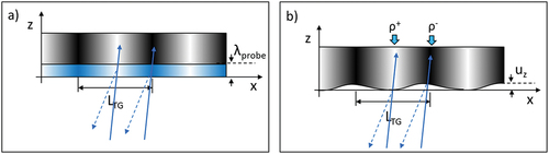10–100 nm. Nevertheless, the EUV TG can also drive surface excitations, which can be of twofold nature, as described in Figure 6. Firstly, the refractive index modulation at the surface $\mathrm{\Delta }{n}_{surf}\left({\lambda }_{probe};\mathrm{\Delta }t\right)$ reflects a spatial modulation of the reflectivity $R$, which can directly lead to backward diffraction (see Figure 6a). $\mathrm{\Delta }{n}_{surf}\left(t,{\lambda }_{probe}\right)$ is typically dominated by electronic excitations in a sample depth roughly comparable with ${\lambda }_{probe}$, similarly to $\mathrm{\Delta }R/R$ data shown in Figure 9e). Secondly, the $\mathrm{\Delta }\rho \left(\mathrm{\Delta }t\right)$ modulation associated with the thermal expansion leads to a spatial modulation of the surface displacement, i.e. a surface wave, with the excited, hot, fringes that are displaced by a thickness $u_z\left(\mathrm{\Delta }t\right)$ with respect to the unexcited, cold, ones. In this case the EUV TG signal is given by the optical path difference between the rays reflected by the peaks and the valleys of the surface wave, as shown schematically in panel b) and extensively discussed in [118]. The time dependent surface displacement $u_z\left(\mathrm{\Delta }t\right)=A_T\left(\mathrm{\Delta }t\right)+{\mathrm{\Sigma }}_i{A}_i{e}^{-\mathrm{\Delta }t/{\tau }_i}cos({\omega }_i\mathrm{\Delta }t)$ contains information on the decaying amplitude of the thermal grating $A_T\left(\mathrm{\Delta }t\right)=A_T{e}^{-\mathrm{\Delta }t/{\tau }_T}$ and on amplitude $A_i$, decay ${\tau }_i$ and angular frequency ${\omega }_i$ of the SAWs and possibly also other kind of collective vibrational modes affecting $u_z\left(\mathrm{\Delta }t\right)$, such as the surface skimming longitudinal waves (SSLW) at the selected value of $k_{TG}$.

Figure 6. a) Backward diffraction (dashed lines) of a probe beam (full lines) from the modulation of surface refractive index (blue area) in a depth comparable with the probe wavelength (${\lambda }_{\text{probe}}$). b) Backward diffraction (dashed lines) of a probe beam (full lines) from the modulation of surface displacement $\left({\text{u}}_{\text{z}}\right)$, ${\rho }^{+}=\rho +\mathrm{\Delta }\rho$ and ${\rho }^{-}=\rho -\mathrm{\Delta }\rho$ indicate denser and more rarefied regions (with $\rho$ the average density and $\mathrm{\Delta }\rho$ its maximum variation), corresponding, respectively to cold and hot regions of the thermal grating.

These two surface contributions are what dictates the efficiency of the backward diffracted signal, ${\eta }_B\left(\mathrm{\Delta }t\right)$, as given in the following equation: Equation 9(9) $\begin{array}{ll}{\eta }_B\left(\mathrm{\Delta }t\right)=& \left[R{\left(2\frac{\pi u_z\left(\mathrm{\Delta }t\right)}{{\lambda }_{probe}}\right)}^{2}cos\left({\theta }_{sig}\right)cos\left({\theta }_{probe}\right)+\mathrm{\Delta }{n}_{surf}^2\left({\lambda }_{probe};\mathrm{\Delta }t\right)/4\right]\\ & \times \xi \left({\sigma }_i,\mathrm{\Delta }{t}_p\right),\end{array}$(9)

(9) $\begin{array}{ll}{\eta }_B\left(\mathrm{\Delta }t\right)=& \left[R{\left(2\frac{\pi u_z\left(\mathrm{\Delta }t\right)}{{\lambda }_{probe}}\right)}^{2}cos\left({\theta }_{sig}\right)cos\left({\theta }_{probe}\right)+\mathrm{\Delta }{n}_{surf}^2\left({\lambda }_{probe};\mathrm{\Delta }t\right)/4\right]\\ & \times \xi \left({\sigma }_i,\mathrm{\Delta }{t}_p\right),\end{array}$(9)

where $\xi \left({\sigma }_i,\mathrm{\Delta }{t}_p\right)$ is the same function as in Equation 8(8) $\xi \left({\sigma }_i,\mathrm{\Delta }{t}_{pump}\right)={\left(1+\frac{2{\sigma }_{probe}^2}{{\sigma }_{pump}^2}+\frac{2{\sigma }_{probe}^2}{L_{int}^2}\right)}^{-\frac{1}{2}}{\left(1+\frac{2{\sigma }_{probe}^2}{{\sigma }_{pump}^2}\right)}^{-\frac{1}{2}}.$(8) , which depends on the space and time overlap between the pulses. We note that in principle $u_z\left(\mathrm{\Delta }t\right)$ and $\mathrm{\Delta }{n}_{surf}$, as well as thickness modulations in thin samples, can contribute to forward diffraction, while modulations in $\mathrm{\Delta }n$ can contribute to backward diffraction. However, our experience suggests that such contributions are typically marginal in EUV TG.

3.3 EUV TG excitation

In the optical regime the photoexcitation mechanisms depend on how the optical photon energy ($E_{opt}$) compares to the plasma frequencies (e.g. in metals), band gaps (e.g. in insulators and semiconductors) and other characteristic energies of the valence band structure (e.g. defect or polaron states). Using EUV pulses the value of $E_{EUV}$ is larger than any of the aforementioned characteristic energies of the investigated samples. The main response of materials to an EUV pump pulse, irrespectively of their dielectric, semiconducting or metallic nature, is sketched in Figure 7a) along with the time profile of the excitation pulse. The first excitation step is the ultrafast generation of a population of hot electrons (panel b), which initially relaxes mainly via electron-electron interactions (panel c) [190,191,220]. The timescale for this energy redistribution process within the electronic subsystem (${\tau }_{e-e}$) is on the 10 fs scale, which is faster than the excitation pulses typically used in EUV TG experiments ($\mathrm{\Delta }t\approx$ 40–60 fs). In this case the concept of impulsive excitation illustrated in Figure 2a does not hold, these dynamics cannot be coherently excited and the information on the initial photoexcitation process is lost, washed out by the ‘convolution’ of the excitation and thermalization processes itself. On a longer timescale (${\tau }_{e-l}\approx$100s of fs) the electronic excitation relaxes into the lattice (panel d), finally resulting in a lattice heating. The TG excitation adds the spatial modulation $L_{TG}$ to these dynamics, since these processes only happen in correspondence of the spatial locations where the interference pattern has a non-zero intensity while nothing happens in the spatial locations of destructive interference (unexcited regions); see Figure 5.

Figure 7. a) Sketch of the EUV TG excitation process: the blue curve depicts an EUV pulse with time duration $\mathrm{\Delta }{\text{t}}_{\text{pump}}\approx$ 10s fs. EUV photons with photon energy ${\text{E}}_{\text{EUV}}$ are mainly absorbed by valence electrons (blue vertical lines in Panel b) and initially generate a population of hot electrons (black dots) and valence band holes (white dots); the valence and conduction bands are represented, respectively, by grey and white parabolic areas. On the 10 fs scale this population relaxes (black wavy downwards arrows in panel c) generating electron-hole pairs across the valence band, which recombines on the 100s fs scale (black downwards arrows in panel d). The EUV TG excitation thus creates an electronic population grating that is relaxing by transferring energy to the lattice. The lattice is hence heated in a spatially periodic way (thermal grating) inducing, e.g. spatially periodic changes in density (via thermal expansion; panel e) or magnetization (panel f). For a moderate EUV excitation level, these gratings evolve in time up to recover the initial (unperturbed) state. In this illustration electronic transitions involving core-hole states are ignored.

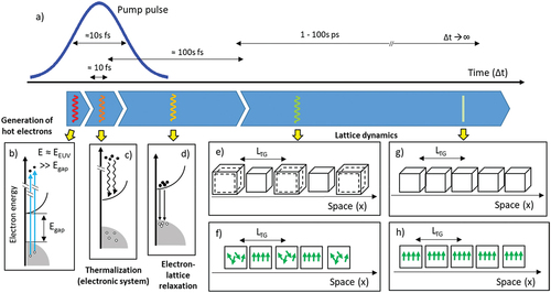
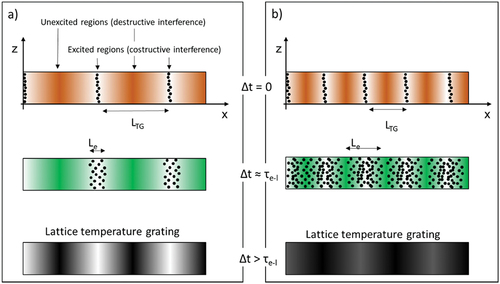
The thermal grating with a given periodicity $L_{TG}$ evolves into a periodic modulation of physical quantities coupled to the temperature, e.g. into a density grating (via thermal expansion; see Figure 7e) and a magnetization grating (via the temperature dependence of the magnetization; see Figure 7f). As long as the electronic diffusion can be neglected, as discussed below, the periodicity of these thermally-induced gratings is the same as the excitation light pattern and they evolve in time following specific dynamics that are monitored by the probe pulse. For moderate EUV excitation intensity the sample returns in the initial (unperturbed) condition at longer times (Figure 7g-h). If this time is shorter than the inverse repetition rate of the pulsed EUV photon source the dynamics can be probed in a stroboscopic fashion. EUV TG experiments were so far performed at low repetition rate FELs (<1 kHz), however, repetition rates in the MHz level are likely exploitable.

This picture assumes that during the initial energy redistribution processes, i.e. over a timescale $\approx {\tau }_{e-l}$, the electron mean free path $L_e\ll L_{TG}$. In this condition the energy transfer from the TG to the electron system and then to the lattice essentially preserves the spatial modulation imposed by the TG itself. This is sketched in Figure 8a for the situation where hot electrons are impulsively generated at $\mathrm{\Delta }t=0$, uniformly along the sample depth and only in correspondence to the maxima of the TG interference. These assumptions are obviously not realistic since, as discussed above, with typical values of $\mathrm{\Delta }{t}_{pump}$ the response of the electronic system is not impulsive and hot electrons are generated in all sample locations proportionally to the magnitude of the interference intensity, which decreases along Z because of the optical absorption of the pump beams. In a realistic situation one should thus imagine this electronic population to be proportional to a sinusoidal modulation (along the coordinate x) and an exponential decay (along the coordinate z). Additionally, at least for moderate excitations, this instantaneously photoexcited electronic population evolving in the fs time-scale should be considered as convoluted with the gaussian temporal profile of the excitation pulse.

Figure 8. Effect of the relative magnitude between the electron mean free path (${\text{L}}_{\text{e}}$) and the TG period (${\text{L}}_{\text{TG}}$). Black dots sketch the excited electrons. Panel a) displays the situation where ${\text{L}}_{\text{TG}}\gg {\text{L}}_{\text{e}}$, no electronic diffusion occurs and the spatial distribution of excited electrons at $\mathrm{\Delta }t=0$ (top picture) is similar to the one observed at $\mathrm{\Delta }t=\text{,}{\tau }_{\text{e}-\text{l}}$ (middle picture), when electron and lattice equilibrate, resulting in a spatial profile of the lattice temperature grating (bottom picture) having essentially the same contrast as the EUV TG. The condition ${\text{L}}_{\text{TG,}}\approx \text{,}{\text{L}}_{\text{e}}$ is illustrated in panel b), at $\mathrm{\Delta }\text{t,}\approx {\tau }_{\text{e}-\text{l}}$ electrons diffuse away from excited to unexcited regions, leading to a lattice temperature grating with the same periodicity but a sizably reduced contrast.

In light of the typical values of electron mean free path in condensed matter [221], this situation is a reasonable approximation of reality as long as the value of $L_{TG}$ is on the order of 10 nm or longer. For shorter values one may expect a tangible electronic diffusion from regions of maximum to minimum TG intensity, which results in a decrease in TG visibility, as illustrated in Figure 8b). Single-digit nm TGs are hardly achievable with EUV excitation; however, these values (or even shorter) could be at reach via X-ray TG. Moreover, high energy ($\approx$ keV) electrons generated by X-rays can have MFP_e substantially longer than those generated by EUV photons [221], therefore the condition $L_{TG}\ll L_e$ could be reached. In this case the photoexcited electrons can move across many fringes of the TG during the initial thermalization process, i.e. before releasing energy to the lattice, with the possible consequence that the nanoscale thermal grating cannot be excited at all, at least not through this photoexcitation mechanism.

3.4 EUV TG with optical probe

The dynamic processes that can be detected in a EUV TG experiment depend on the time duration of the probe pulse and on how it couples with the refractive index variation induced by the pump (Equation 5(5) $\begin{array}{ll}n\left({\lambda }_{probe};x,z,\mathrm{\Delta }t\right)& =n\left({\lambda }_{probe}\right)+\mathrm{\Delta }n\left({\lambda }_{probe};\mathrm{\Delta }t\right)\\ & \times cos\left(2\pi x/L_{TG})exp(-z/L_{abs}\right)\end{array}$(5) ). In Figure 9a) we show the typical response observed by using an optical pulse of wavelength ${\lambda }_{probe}$ = 390 nm diffracted from a EUV-induced grating of sufficiently long periodicity $L_{TG}\sim$ 280 nm (see Equation 4(4) $L_{TG}\left[sin\left({\theta }_{sig}\right)+sin\left({\theta }_{probe}\right)\right]={\lambda }_{probe},$(4) ).

Figure 9. a) EUV TG signal with optical probe from a BK7 glass sample [218]; note the broken scale in the horizontal axis to separate the fast response due to electronic signal around $\mathrm{\Delta }\text{t,}=0$ and the slower modulations due to phonon propagation. The blue curve is a gaussian peak with a FWHM of $\approx$ 160 fs, compatible with the experimental resolution, while the red curve is an exponential decay with time constant of $\approx$ 250 fs, on the same order as ${\tau }_{\text{e}-\text{l}}$. Panel b) sketches the electronic structure at $\mathrm{\Delta }t<\text{,}0$, that is the one of the unperturbed sample. All probing optical photons (red wavy arrows) are transmitted through the sample because ${\text{E}}_{\text{opt,}}<\text{,}{\text{E}}_{\text{gap}}$. Panel c) displays the effect of EUV photons (blue wavy arrows), mainly occurring within the time duration of the pulses ($-\mathrm{\Delta }{\text{t}}_{\text{pump}}/2\text{,,}<\mathrm{\Delta }\text{t,}<\mathrm{\Delta }{\text{t}}_{\text{pump}}/2\text{,,}$) and resulting in the promotion of electrons from the valence to the high energy portion of the conduction band (straight vertical blue arrows); note the broken vertical scale. These electrons thermalize on a timescale shorter than the typical values of $\mathrm{\Delta }{\text{t}}_{\text{pump}}$ employed so far in EUV TG experiments (black wavy downward arrows). Optical photons can now be strongly absorbed by intraband transitions (red vertical lines in panels c) and d), until these states relax; see panel d). Panel e) compares EUV TG (black dots) and transient reflectivity signals (red and blue dots; green lines are guide for the eyes) from a SiN sample. The EUV fluence for the TG data was 0.5 mJ/cm² while for transient reflectivity was 8 mJ/cm² (red dataset) and 35 mJ/cm² (blue dataset). The signal to noise ratio is much higher for TG, despite the lower excitation fluence, while the dynamics was essentially the same (see also dashed vertical lines). Panel e) is adapted from [219].

3.4.1 Electronic response

In this specific example the pump pulses ($\mathrm{\Delta }{t}_{pump}\approx$ 100 fs, ${\lambda }_{pump}=$ 12.7 nm) are crossing at $2\theta =$2.6° and the probe is incident at ${\theta }_{probe}=$ 45°. The sample is an optical glass (BK7) transparent to the probe, i.e. the energy bandgap ($E_{gap}$) is larger than the probe photon energy ($E_{opt}=$ 3.1 eV in this case) and the refraction index is purely real. In the unexcited sample the probe beam is not diffracted because TG, therefore the signal is zero for $\mathrm{\Delta }t<0$. At the arrival time of the EUV excitation, hot electrons with energies comparable to $E_{EUV}$ $\approx$ 10–100 eV are removed from the valence band, leaving holes behind them. These represent new absorption channels for the optical probe, via intraband transitions [190,222], as sketched in Figure 9c). This significantly changes $n\left({\lambda }_{probe};\mathrm{\Delta }t\approx 0\right)$, both by inducing an imaginary part and by varying the value of the real part, i.e.: $\partial n\left({\lambda }_{probe};\mathrm{\Delta }t\right)/\partial {\rho }_e=a_e\ne 0$, with ${\rho }_e$ the density of the electronic excited states; the presence of excited electrons in the conduction band may marginally contribute to the refractive index variation. The transient changes are modulated in space, following the modulation of the TG (see Equation 5(5) $\begin{array}{ll}n\left({\lambda }_{probe};x,z,\mathrm{\Delta }t\right)& =n\left({\lambda }_{probe}\right)+\mathrm{\Delta }n\left({\lambda }_{probe};\mathrm{\Delta }t\right)\\ & \times cos\left(2\pi x/L_{TG})exp(-z/L_{abs}\right)\end{array}$(5) ), resulting in a sizable value of $\mathrm{\Delta }n\left({\lambda }_{probe};\mathrm{\Delta }t\right)\sim a_e\mathrm{\Delta }{\rho }_e\left(\mathrm{\Delta }t\right)$, with ${\rho }_e\left(\mathrm{\Delta }t\right)$ the time-dependent variation of ${\rho }_e$, and thus in a tangible signal (see Equation 6(6) ${\eta }_F\left(\mathrm{\Delta }t\right)=\frac{I_{sig}}{I_{probe}}={\left|\mathrm{\Delta }n\left({\lambda }_{probe};\mathrm{\Delta }t\right)\right|}^{2}F\left({\lambda }_i,{\theta }_i,L_i,d\right)\xi \left({\sigma }_i,\mathrm{\Delta }{t}_{pump}\right),$(6) ). The thermalization dynamics of hot electrons within the electronic subsystem is faster than $\mathrm{\Delta }{t}_{pump}$, as sketched in Figure 7, therefore this dynamics cannot be coherently excited (see Figure 2) and is washed out by the ‘convolution’ of the excitation and thermalization processes. This reflects into a rise time of the EUV TG signal that is substantially given by the time profile of the pulses, i.e. by the gaussian function shown in Figure 9a) (blue line), representing the time resolution of the experiment. This signal rise reflects the sensitivity to the presence of electronic excitations even if any dynamics can be directly detected. Note that beside short pump pulses, a short probe pulse is needed as well (or a more sophisticated approach that provides control on other parameters, e.g. the phase [213]). The subsequent relaxation of the population of excited electronic states into the thermal excitation of the lattice instead occurs in the ${\tau }_{e-l}\approx$ 100s of fs scale and leads to the signal decay shown in Figure 9a) (red line), which reflects the disappearance of such populations (Figure 9d). The EUV TG signal arising from these electronic dynamics has not a substantially different nature with respect to an EUV-pump/optical-probe signal, since electrons cannot ‘feel’ the spatial structure of the grating (see Figure 8). Figure 9e) shows a comparison between the EUV TG signal and the transient reflectivity pump-probe signal from a Si₃N₄ sample, which detects the relative variation of optical reflectivity ($\mathrm{\Delta }R/R$) induced by the EUV pump. The dynamics of these two signals are essentially the same, since the same $\mathrm{\Delta }n\left({\lambda }_{probe};\mathrm{\Delta }t\right)$ variations are responsible for a change in R [219]. This comparison also illustrates the intrinsic advantage of the TG method as background free technique. Indeed, the TG signal is emitted in a direction where other spurious emissions are absent, allowing us to detect a small signal over a zero background, with a S/N only limited by the shot noise of the detector. On the contrary, the $\mathrm{\Delta }R/R$ signal requires the determination of small variations (% or sub-%) over a large signal due to the reflected probe; the same consideration holds for transient transmission or scattering experiments. Despite the low efficiency of the TG process, its large S/N allows it to use lower pump intensities guaranteeing lower sample damage and conditions closer to the room temperature ones. Note that TG data shown in Figure 9e) have been collected at a fluence of 0.5 mJ/cm² while the two $\mathrm{\Delta }R/R$ datasets at 8 and 35 mJ/cm²; the S/N of TG is evidently better even though the fluence is lower by more than one order of magnitude.

When $E_{gap}<E_{opt}$ the optical probe photons are absorbed and promote valence electrons into the conduction band, in this case the electrons removed from the valence band by the EUV excitation induce a significant reduction of optical absorption, thus again leading to a significant change in $\mathrm{\Delta }n\left({\lambda }_{probe};\mathrm{\Delta }t\right)$. EUV TG signals with optical probes were observed also from optically opaque materials. In metals, where there is no bandgap and the optical refractive index has a strong imaginary component, one can expect that the initial excitation is much less effective but still appreciable since the electronic structure of real metals is featured by bands that can be disturbed by the EUV excitation [190]. However, this is just an expectation since at the time of writing we do not have data from metallic samples excited by EUV TG and probed by optical photons.

3.4.2 Collective lattice response (bulk)

After the decay of electronic excitations, the EUV TG signal is not zero, as visible from Figure 9a) since the energy transfer to the lattice has generated temperature ($T$) and density ($\rho$) gratings capable of diffracting the probe (see Equation 6(6) ${\eta }_F\left(\mathrm{\Delta }t\right)=\frac{I_{sig}}{I_{probe}}={\left|\mathrm{\Delta }n\left({\lambda }_{probe};\mathrm{\Delta }t\right)\right|}^{2}F\left({\lambda }_i,{\theta }_i,L_i,d\right)\xi \left({\sigma }_i,\mathrm{\Delta }{t}_{pump}\right),$(6) ), provided that the density and temperature dependencies of the optical refractive index at the probe’s wavelength are not vanishing, i.e.: $\partial n\left({\lambda }_{pr};\mathrm{\Delta }t\right)/\partial \rho =a_{\rho }\ne 0$ and $\partial n\left({\lambda }_{pr};\mathrm{\Delta }t\right)/\partial T=a_T\ne 0$. Right after the electronic relaxation the sample lattice is characterised by alternate compressed-rarefied regions and hot-cold regions, as illustrated in Figure 10(a,b), respectively. The dynamics of these gratings develop on much longer timescales, as shown in Figures 7 and 8. Over such timescales the difference between optical and EUV excitation of the TG is no longer relevant and, just like in optical TG, these dynamics contain the relevant information on collective lattice excitations at a given value of $L_{TG}$. In the example shown in Figures 9 and 10, the EUV TG signal modulations at 50 ps period, corresponding to the $\omega =$ 0.135 THz peak labelled as LA in the Fourier-spectrum shown in panel c), represent the elastic response due to the propagation of two counter-propagating longitudinal acoustic (LA) phonons with wavevector $k_{LA}=\pm k_{TG}$. These phonons are a consequence of the electron-lattice interaction and of thermal expansion, which converts the thermal grating into a density grating. After a time interval $t_{LA}/2=\pi /\left|k_{LA}\right|c_{LA}=L_{TG}2c_{LA}$ (where $c_{LA}$ = 6048 m/s in this case [218]) the elastic restoring forces equilibrate the density throughout the sample and, after another time interval $t_{LA}/2$, they compress/expand the regions that were previously rarefied/compressed and so on; see Figure 10a). This induces a periodic modulation of $\mathrm{\Delta }n\left({\lambda }_{probe};\mathrm{\Delta }t\right)\sim a_{\rho }\mathrm{\Delta }\rho \left(\mathrm{\Delta }t\right)$, with $\mathrm{\Delta }\rho \left(\mathrm{\Delta }t\right)$ the time dependent difference in the density of compressed and rarefied zones. The resulting modulation in $\mathrm{\Delta }t$ of the EUV TG signal will last as long as the counter propagating phonons do not naturally decay, e.g. by phonon-phonon interactions, or move away from the excitation region. The latter happens after a time interval $t_{exit}=\sigma /c_{LA}$, with $\sigma$ the size of the interaction region along the phonon propagation direction (x axis; see Figure 4). For typical values of $\sigma \approx$ 100 μm one has $t_{exit}\approx$ 100 ns, which is significantly larger than the maximum range in $\mathrm{\Delta }t$ usually exploitable by EUV TG instruments (a few ns). Data reported in Figures 9 and 10 do not show evident phonon decay in the probed $\mathrm{\Delta }t$ range (up to 0.5 ns), as expected for this specific sample at the relatively long value of $L_{TG}$ = 277 nm used here. A slow signal decay, highlighted by the green line in Figure 10c) can be ascribed to the decay of the temperature grating due to heat transport from hot (constructive interference fringes) to cold regions (destructive interference fringes) of the grating; see Figure 10b). This behaviour agrees with the expected magnitude of the thermal decay time: ${\tau }_T\approx {L^2}_{TG}/4{\pi }^2{D}_T\approx$ 4 ns in the present case.

Figure 10. a) Same data as Figure 9a [218] the green line in the long $\mathbf{\Delta }\mathbf{t}$ range is the slow decay ascribable to heat transport. The left image in panel b) sketches the thermal grating (temperature modulation) generated by the relaxation of electronic population grating into the lattice. Yellow arrows indicate the heat flow from hotter to colder regions. The amplitude of the thermal grating reduces on increasing $\mathrm{\Delta }\text{t}$ up to vanishing for $\mathrm{\Delta }\text{t,}\to \text{,}\mathrm{\infty }$ (middle and right pictures). The left picture in panel c) is the density grating initially generated by thermal expansion, which time evolution is driven by elastic restoring forces (sketched by yellow arrows) that restore a uniform density after half of the phonon period (${\text{t}}_{\text{LA}}/2$) and after another ${\text{t}}_{\text{LA}}/2$ time interval lead to the compression of previously rarefied zones; see red arrows connecting the pictures in panel c) with the signal modulations in panel a). This time dependent density modulation is finally washed out by phonon decay (not visible in the probed $\mathrm{\Delta }\text{t}$ range). Panel d) is the Fourier transform of the EUV TG signal modulations.

In Figure 10b) we illustrated the conventional thermal relaxation process, however, in some cases heat dynamics may include thermal waves, where heat bounces back and forth from hot to cold regions, similarly to the density variations related to the phonon dynamics sketched in Figure 10a) [132,223,224].

The Fourier spectrum of Figure 10c) shows an additional peak at $\omega =$ 0.074 THz, labelled as SAW, which corresponds to the Rayleigh SAW and which will be discussed in detail in section 3.3.3.

3.4.3 Collective lattice response (surface)

The initial electronic excitation grating can generate a modulation of the surface’s refractive index, while its subsequent relaxation into $T$ and $\rho$ gratings can result into a modulated surface displacement; both modulations can result into diffraction of the probe (see Equation 9(9) $\begin{array}{ll}{\eta }_B\left(\mathrm{\Delta }t\right)=& \left[R{\left(2\frac{\pi u_z\left(\mathrm{\Delta }t\right)}{{\lambda }_{probe}}\right)}^{2}cos\left({\theta }_{sig}\right)cos\left({\theta }_{probe}\right)+\mathrm{\Delta }{n}_{surf}^2\left({\lambda }_{probe};\mathrm{\Delta }t\right)/4\right]\\ & \times \xi \left({\sigma }_i,\mathrm{\Delta }{t}_p\right),\end{array}$(9) ). Figure 11a a) shows data acquired on BK7 glass in backward diffraction, simultaneously to the data presented in Figures 9 and 10 [218]. The signal contains the same information on the ultrafast electronic decay and on the slow thermal decay, while the phonon modulations differ from the ones measured in forward scattering. Figure 11b b) shows the Fourier spectrum of the backward diffracted data. Comparing it to panel c) of Figure 10, we observe that the peak at $\omega =$ 0.074 THz, which matches the expected SAW frequency, is much more prominent, while the LA peak at $\omega =$ 0.135 THz that dominates the signal in transmission is still observable.

Figure 11. a) EUV TG signal with optical probe collected in backward diffraction from a BK7 glass sample [218]; data were acquired in parallel with those shown in Figures 9a and 10a. Note the broken scale in the horizontal axis to separate the fast response due to electronic signal around $\mathrm{\Delta }\text{t,}=0$ and the slower modulations due to phonon propagation. The blue curve is a gaussian peak with a FWHM of 160 fs, compatible with the experimental resolution, while the red curve is an exponential decay with time constant of 200 fs, on the same order as ${\tau }_{\text{e}-\text{l}}$. Panel b) is the Fourier transform of the EUV TG signal modulations; SAW, LA(k_TG) and LA(k_z) indicate the signal modulations due to, respectively, surface acoustic waves, longitudinal acoustic phonons propagating along ${\text{k}}_{\text{TG}}$ and along ${{\text{k}}_{\text{z}}}^{-}$ (see text).

Surface and bulk acoustic waves are not commonly observed simultaneously. In the optical regime, experiments are typically performed in samples that are either transparent or opaque at both pump and probe wavelengths. In the first case, both signals are in principle visible because the surface displacement modulates the optical path across the sample. However, the bulk signal grows quadratically with sample thickness, while the surface signal is only attenuated while propagating through the sample. Thus, typically only bulk acoustic waves are observed. In the second case the pulses do not propagate in the sample volume and the signal, measured necessarily in backward diffraction, is dominated by the SAW contribution. Here, the sample is opaque to the pump pulse and transparent to the probe. The bulk signal is generated over an optimal sample length and surface and bulk contributions can be comparable in forward diffraction. The presence of the bulk signal in back scattering in this specific case can instead be explained by the reflection of the forward scattered signal on the posterior surface of the sample being detected by the reflection CCD [218].

In backward diffraction an additional peak at $\omega =$ 0.297 THz was observed (labelled as LA(k_z) in Figure 11b, which is also a consequence of the thin excitation volume due to the strong absorption of the EUV pump. The phonons launched by the EUV TG have a well-defined value of $k_{exc}$ only along the surface, while a broad phonon spectrum can be excited along the perpendicular direction ($k_z$). The phase matching conditions for the probe beam to be diffracted by the acoustic excitations are satisfied both for ${k_z}^{+}=$ 0, corresponding to forward diffraction and for ${k_z}^{-}=2n\left({\lambda }_{probe}\right)k_{probe}\sqrt{1-{k_{TG}}^2/{(2n\left({\lambda }_{probe}\right)k_{probe})}^2},$ which is associated with backward diffraction and with an expected modulation frequency of backscattered phonons of $\omega =2n\left({\lambda }_{probe}\right)c_{LA}{k}_{probe}=$ 46.9 GHz, which well matches the observed value [218].

3.4.4 Molecular vibrations

Figures 9, 10 and 11 show exemplificative cases of EUV TG excitation probed by an ultrafast optical pulse, where the dynamics is dominated by the relaxation of valence band electronic excitations, (bulk) LA phonons, SAWs and thermal decay. These are not all the sample responses that one can measure in a EUV TG experiment. Actually, any dynamics that can be excited by the EUV pump and that affect $n\left({\lambda }_{probe}\right)$ can be monitored by EUV TG. As an example, other dynamic processes that may induce a modulation of the optical refractive index are Raman modes, i.e. atomic vibrations within a molecule, either isolated or constituting the asymmetric unit of a solid.

Figure 12 illustrates the difference between LA and Raman modes in the case of a unidimensional crystal with an asymmetric unit of two atoms having different mass, $m_1$ and $m_2$. LA modes are the motion of the barycenter of the asymmetric unit with respect to its rest position. In the proposed example, if the LA phonon displaces the two particles from their rest positions ($x_1$ and $x_2$) of the same quantity A, then the coordinate of the barycenter can be expressed as: $R{}^{\prime }=\left[m_1\left(x_1+A\right)+m_2\left(x_2+A\right)\right]/\left(m_1+m_2\right)=R+A$, with R=$(m_1{x}_1+m_2{x}_2)/\left(m_1+m_2\right)$. Assuming the total mass of the asymmetric unit as contained in a sphere of radius r, then the effect of the LA wave is to move this sphere from its original position to a new one offset by A. For A < R this yields to $\mathrm{\Delta }\rho /\rho \approx 3A/4R$. Optical phonons instead are defined as the displacement of the atoms (a₁ and a₂) with respect to the barycentre, which is located at $R{}^{\prime }=\left[m_1\left(x_1+a_1\right)+m_2\left(x_2-a_2\right)\right]/\left(m_1+m_2\right)$. Calling $c$ the total length variation of the bound then the quantities $a_1$ and $a_2$ can be written as $a_1=m_{2}c/\left(m_1+m_2\right)$ and $a_2=m_{1}c/\left(m_1+m_2\right)$ that, when inserted into the formula for the centre of mass, yields R=R’. Optical phonons are thus not associated with a density variation, but, changing the interatomic distance, may alter the dipole moment of the molecule. These changes can be actually read by an optical probe via RLS.

Figure 12. a) Effect of a LA phonon polarised along X in an unidimensional crystal with an asymmetric unit made out of two atoms (shaded orange and pink circles). Dotted circles represent the equivalent reference volume for the asymmetric unit at rest. LA phonons displace all the atoms in the same direction by A. This causes the equivalent volume of the system (here sketched as solid circles) to move in-and-out of the reference volume, causing the periodic density change. b) Optical phonons move the atoms far from each other by the quantities a₁ and a₂, which are inversely proportional to their masses. This motion does not change the position of the equivalent mass sphere (see vertical dotted lines for reference), thus maintaining the density, while changing the relative positions of the two atoms (here the dotted circles represent the rest positions of the two atoms).

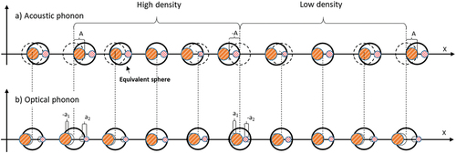
Raman modes can be stimulated impulsively, e.g. via displacive excitation of coherent phonons (DECP). This mechanism takes place only in absorbing materials where the absorbed photons can generate an electronic cloud. Electron-electron scattering leads to an ultrafast equilibration of the electron gas far from the equilibrium position occupied in the ground state. This induces a force that, similarly to a mass-spring system, causes the oscillation of nuclei [225,226]. Refractive index changes due to atomic displacements along the coordinates of the nuclei is given by: Equation 10(10) $\mathrm{\Delta }{n}_{Raman}\left({\lambda }_{probe};\mathrm{\Delta }t\right)/n=A{e}^{-\beta \mathrm{\Delta }t}+B{e}^{-\gamma \mathrm{\Delta }t}\left(cos\left(\mathrm{\Omega \Delta }t\right)-\frac{\beta -\gamma }{\mathrm{\Omega }}sin\left(\mathrm{\Omega \Delta }t\right)\right),$(10)

(10) $\mathrm{\Delta }{n}_{Raman}\left({\lambda }_{probe};\mathrm{\Delta }t\right)/n=A{e}^{-\beta \mathrm{\Delta }t}+B{e}^{-\gamma \mathrm{\Delta }t}\left(cos\left(\mathrm{\Omega \Delta }t\right)-\frac{\beta -\gamma }{\mathrm{\Omega }}sin\left(\mathrm{\Omega \Delta }t\right)\right),$(10)

where $\beta$ is the electron relaxation rate, $\gamma$ the relaxation rate of the Raman mode and $\omega$_Raman the Raman frequency, with $\mathrm{\Omega }=\sqrt{{\omega }_{Raman}^2-{\gamma }^2}$. For $\beta \gg \gamma$ the time dependence is sinusoidal and $\mathrm{\Delta }{n}_{Raman}\left({\lambda }_{probe};\mathrm{\Delta }t\right)/n$ decreases, while when $\beta \approx \gamma$ the sinusoidal term can be dropped and cosinusoidal oscillations can be observed; see [225] for additional details. Only Raman modes of specific symmetries can be excited by the DECP mechanism [225,226].

EUV TG can add a given spatial modulation to the DECP excitation mechanism and the optical probe can couple to the stimulated Raman mode through the optical refractive index variation (Equation 10(10) $\mathrm{\Delta }{n}_{Raman}\left({\lambda }_{probe};\mathrm{\Delta }t\right)/n=A{e}^{-\beta \mathrm{\Delta }t}+B{e}^{-\gamma \mathrm{\Delta }t}\left(cos\left(\mathrm{\Omega \Delta }t\right)-\frac{\beta -\gamma }{\mathrm{\Omega }}sin\left(\mathrm{\Omega \Delta }t\right)\right),$(10) ), thus leading to the observation of Raman oscillations in the $\mathrm{\Delta }t$ dependence of the EUV TG signal, as shown in Figure 13a). In this case the sample was a BGO crystal under the same experimental conditions used to obtain the data in Figures 9, 10 and 11. The same signal was observed also by Rouxell and co-workers in the experiment where the capability to excite TG with hard X-rays was demonstrated [227]. Here they generated a hard X-ray TG with $L_{TG}=$ 770 nm (Figure 13b); we recall that the EUV TG data shown in Figure 13a, was collected at $L_{TG}=$277 nm. The Fourier transforms of EUV and X-ray TG signal are reported in Figure 13c, and both show a clear peak at $\omega =$ 16.3 THz. The absence of dispersion in the detected angular frequency as a function of $L_{TG}$ is typically expected for optical phonons. This experimental observation brings to two main conclusions: i) the DECP mechanism is effective for both EUV and hard X-ray light. ii) since hard X-rays penetrate several µm’s into the sample, the Raman modes excited in a sample depth of about $L_{abs,pump}\approx$ 100 nm are essentially identical to those excited in the bulk.

Figure 13. Optically probed EUV TG (panel a); adapted from [218]) and hard X-ray signal (panel b); adapted from [227]) from a BGO sample. c) Fourier transform of these oscillatory signals, black and red curves correspond, respectively, to EUV and X-ray TG.

3.4.5 Core-hole excitations

All EUV TG data shown so far (Figures 9–11 and 13a) were collected using EUV excitation wavelengths not resonant with core absorption edges of the investigated materials. Therefore, the EUV-induced electronic excitation involves only valence excitations, as sketched in Figure 7b. This aspect is irrelevant as long as one is interested in the thermoelastic response, since electronic excitations are in practice only used to ‘translate’ the electromagnetic interference pattern into a thermal grating, whose dynamics develop in the ps scale. All the details of the fs dynamics of the initially excited electronics states are of little importance in this context. However, EUV photons could stimulate core electronic transitions, resulting in excited core-hole states with lifetimes typically limited to the few fs scale by Auger decay, as shown in Figure 14a. While the direct detection of the dynamics of these states is limited by the current setup and pulse duration, indirect information on these processes can be obtained by a proper modelling of ${\tau }_{e-e}$ and ${\tau }_{e-l}$, the latter occurring in the 100s of fs range easily accessible with the available EUV TG instruments. Figure 14 reports the main results of an EUV TG experiment that exploited core-hole resonances [228]. EUV TG data were collected from a thin silicon nitride (Si₃N₄) sample by varying ${\lambda }_{pump}$ in the 14.6–10.8 nm range, i.e. across the silicon L-edge (Figure 14c) and $\theta$ was varied at the same time to keep $L_{TG}$ fixed at 270 nm (see Equation 2(2) $L_{TG}={\lambda }_{pump}/\left[2sin\left(\theta \right)\right].$(2) ). A clear difference in ${\tau }_{e-l}$ as a function of ${\lambda }_{pump}$ was observed, as displayed in Figure 14b. The analysis of the EUV TG signal as a function of ${\lambda }_{pump}$ revealed a slower relaxation at longer ${\lambda }_{exc}$, and the interband Auger coefficients at high electronic density and temperature were inferred from such wavelength dependence (Figure 14c).

Figure 14. a) EUV TG excitation at photon energy (E_EUV) resonant with a core-hole state (E_C), in this case the EUV photon can promote electrons both from the core level and from the valence band (blue vertical arrows), the latter relaxes (wavy downwards arrow) within $\mathrm{\Delta }{\text{t}}_{\text{pump}}$. b) EUV TG signal with optical probe from a Si₃N₄ sample, at fixed ${\text{L}}_{\text{TG}}$=270 nm and collected using ${\lambda }_{\text{pump}}=$12.28 nm (below the absorption edge; black circles) and ${\lambda }_{\text{pump}}=$11.87 nm (above the absorption edge; red circles); full lines through the experimental data are best fits. c) Black dots are the values of ${\tau }_{\text{e}-\text{l}}$, extracted from the EUV TG waveform, while the blue curve is the measured EUV absorption of Si₃N₄ across the L-edge of silicon. Panels b) and c) adapted from [228].

This represents a first step towards the realisation of multidimensional FWM spectroscopies with both time and energy resolution, and highlights the practical convenience of using TG as a methodological benchmark. Indeed, TG schemes had a key role in the development of advanced spectroscopies in the optical domain. The analysis of FWM signals in TG-like experiments with time resolution beyond the limit dictated by Auger decay could provide information, e.g. on correlations between different atomic species and on ultrafast electronic dynamics with elemental specificity [229–231]. Though theoretically evaluated, EUV/X-ray FWM experiments with enough time resolution and this level of complexity were not carried out yet. As a matter of fact, although broadly tunable and multi-color pulses of the required pulse duration may be in principle available at FELs [232–235], the current setups capable of exploiting FEL pulses in a wave-mixing scheme introduce insuperable technical limitations, such as wavefront tilting or timing jitter, that ultimately spoil the experimental resolution. Different concepts to overcome these limitations can be envisioned, both from the machine and the experimental setup perspective, and will be briefly discussed later on.

3.5 EUV TG with EUV probe

The use of EUV pulses in principle allows to generate TGs with values of $L_{TG}$ in the sub-100 nm range. However, optical probes cannot see these gratings, since Equation 4(4) $L_{TG}\left[sin\left({\theta }_{sig}\right)+sin\left({\theta }_{probe}\right)\right]={\lambda }_{probe},$(4) cannot be fulfilled for ${\lambda }_{probe}>2L_{TG}$. Besides valuable alternatives like ultrafast electron bunches [216], the natural probe for ultrafast and nanoscale EUV TGs is a third, time-delayed, ultrafast EUV pulse.

3.5.1 Refractive index at EUV and X-ray wavelengths

Analogously to the discussion made above for optical vs EUV excitation, the coupling between the EUV probe and the material is weakly dependent on the nature (metallic, dielectric or semiconducting) of the specimen itself, since the refraction index at EUV wavelengths is similar in any material and can be cast in the form: Equation 11(11) $n(\lambda )=1-\delta +i\beta ,with\delta =\frac{(\rho r_e{\lambda }^2)}{2\pi }{f}^{\prime }(\omega )and\beta =\frac{(\rho r_e{\lambda }^2)}{2\pi }{f}^{\prime \prime }(\omega )$(11)

(11) $n(\lambda )=1-\delta +i\beta ,with\delta =\frac{(\rho r_e{\lambda }^2)}{2\pi }{f}^{\prime }(\omega )and\beta =\frac{(\rho r_e{\lambda }^2)}{2\pi }{f}^{\prime \prime }(\omega )$(11)

where r_e is the classical electron radius and f’($\omega$) and f’’($\omega$) are, respectively, the real and imaginary part of the forward scattering cross section: Equation 12(12) $f\left(\omega \right)={\sum }_s\frac{g_s{\omega }^2}{{\omega }^2-{\omega }_s^2+i{\gamma }_s\omega }$(12)

(12) $f\left(\omega \right)={\sum }_s\frac{g_s{\omega }^2}{{\omega }^2-{\omega }_s^2+i{\gamma }_s\omega }$(12)

where $\omega =2\pi c/\lambda$ is the angular frequency of the light, g_s the oscillator strength, Ω_s the resonant frequency and $\gamma$_s the damping rate of the s^th bound electron [236]. This textbook model is based on atomic scattering factors and considers all the electrons to be independent, therefore it does not contemplate the existence of electronic band structures. This is of course a crude approximation but it is effective to illustrate in a simple way a general behaviour. Equation 11(11) $n(\lambda )=1-\delta +i\beta ,with\delta =\frac{(\rho r_e{\lambda }^2)}{2\pi }{f}^{\prime }(\omega )and\beta =\frac{(\rho r_e{\lambda }^2)}{2\pi }{f}^{\prime \prime }(\omega )$(11) and Equation 12(12) $f\left(\omega \right)={\sum }_s\frac{g_s{\omega }^2}{{\omega }^2-{\omega }_s^2+i{\gamma }_s\omega }$(12) highlight a linear dependence on $\rho$ and a dependence on $\omega$ given by the sum of damped harmonic oscillator functions, whose parameters (g_s, ${\omega }_s$ and $\gamma$_s) are essentially determined by the electronic properties of the atomic species present in the sample. The function $f\left(\omega \right)$ is featured by strong dispersions of $\delta$ and $\beta$ when $\omega \approx {\omega }_s$ and smoother dependencies otherwise, as illustrated by the black solid curves in Figure 15a; in this plot we exaggerated the amplitudes of the dispersions for illustrative purposes. In this exemplificative case, we considered two resonances with g₁ = 3, g₂ = 1, ${\lambda }_1=2\pi c/{\omega }_1=20$ nm, ${\lambda }_2=2\pi c/{\omega }_2=80$ nm, ${\gamma }_1=3\ast {10}^3$ THz, ${\gamma }_2=2\ast {10}^3$ THz and $\rho =4\ast {10}^{28}$ e⁻/cm³.

Figure 15. a) Real black line) and imaginary part red line) of the EUV refraction index as a function of,from Equations 10-12, by assuming two electronic transitions (see text for info on the employed parameters). Note the inverse logarithmic horizontal scale in all panels. The refractive index amplitude $(|1-\delta +i\beta |)$ is displayed in panel b), the dotted horizontal line indicates the value of unity and the vertical blue arrow highlights the condition $|1-\delta +i\beta |=1$. c) Dependence of $\mathrm{\Delta }{n}_{\rho }$ (Equation 14(14) $\frac{\partial n\left(\lambda \right)}{\partial \rho }\mathrm{\Delta }\rho =\mathrm{\Delta }{n}_{\rho }\left(\lambda \right)=\left(\frac{r_e{\lambda }^2}{2\pi }f{}^{\prime }\left(\omega \right)+\frac{i{r}_e{\lambda }^2}{2\pi }f{}^{\prime \prime }\left(\omega \right)\right)\mathrm{\Delta }\rho =\left(\delta +i\beta \right)\frac{\mathrm{\Delta }\rho }{\rho }$(14) ) and $\mathrm{\Delta }{n}_{\gamma }$ (Equation 16(16) $\begin{array}{ll}{\sum }_s\frac{\partial n(\lambda )}{\partial {\gamma }_s}\mathrm{\Delta }{\gamma }_s=& \mathrm{\Delta }{n}_{\gamma }(\lambda )\\ =& -\frac{\rho r_e{\lambda }^2}{2\pi }{\sum }_s(\frac{2g_s{\gamma }_s{\omega }^4({\omega }_s^2-{\omega }^2)}{{(({\omega }_s^2-{\omega }^2)+{\gamma }^2{\omega }^2)}^2}+i\frac{g_s{\omega }^3(({\omega }_s^2-{\omega }^2)-{\gamma }^2\omega )}{{(({\omega }_s^2-{\omega }^2)+{\gamma }^2{\omega }^2)}^2})\end{array}$(16) ) on $\lambda$; note the logarithmic vertical scale. $\mathrm{\Delta }{n}_{\gamma }$ is more sizable approaching the resonances, as highlighted by the greenish shaded areas, while are in genera l larger except when (highlighted by the blue arrow). Panel d) is the corresponding trend of the peak at 35 nm reflects the zero of Equation 14(14) $\frac{\partial n\left(\lambda \right)}{\partial \rho }\mathrm{\Delta }\rho =\mathrm{\Delta }{n}_{\rho }\left(\lambda \right)=\left(\frac{r_e{\lambda }^2}{2\pi }f{}^{\prime }\left(\omega \right)+\frac{i{r}_e{\lambda }^2}{2\pi }f{}^{\prime \prime }\left(\omega \right)\right)\mathrm{\Delta }\rho =\left(\delta +i\beta \right)\frac{\mathrm{\Delta }\rho }{\rho }$(14) , which corresponds to the condition (blue arrow in panel c)).

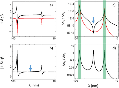
The variations of $n\left(\lambda \right)$ can be described as: Equation 13(13) $\mathrm{\Delta }n\left(\lambda \right)=\frac{\partial n}{\partial \rho }\mathrm{\Delta }\rho +{\sum }_s\frac{\partial n}{\partial {\omega }_s}\mathrm{\Delta }{\omega }_s+{\sum }_s\frac{\partial n}{\partial {\gamma }_s}\mathrm{\Delta }{\gamma }_s+\sum _s\frac{\partial n}{\partial g_s}\mathrm{\Delta }{g}_s$(13)

(13) $\mathrm{\Delta }n\left(\lambda \right)=\frac{\partial n}{\partial \rho }\mathrm{\Delta }\rho +{\sum }_s\frac{\partial n}{\partial {\omega }_s}\mathrm{\Delta }{\omega }_s+{\sum }_s\frac{\partial n}{\partial {\gamma }_s}\mathrm{\Delta }{\gamma }_s+\sum _s\frac{\partial n}{\partial g_s}\mathrm{\Delta }{g}_s$(13)

The three terms of Equation 13(13) $\mathrm{\Delta }n\left(\lambda \right)=\frac{\partial n}{\partial \rho }\mathrm{\Delta }\rho +{\sum }_s\frac{\partial n}{\partial {\omega }_s}\mathrm{\Delta }{\omega }_s+{\sum }_s\frac{\partial n}{\partial {\gamma }_s}\mathrm{\Delta }{\gamma }_s+\sum _s\frac{\partial n}{\partial g_s}\mathrm{\Delta }{g}_s$(13) can be developed to give: Equation 14(14) $\frac{\partial n\left(\lambda \right)}{\partial \rho }\mathrm{\Delta }\rho =\mathrm{\Delta }{n}_{\rho }\left(\lambda \right)=\left(\frac{r_e{\lambda }^2}{2\pi }f{}^{\prime }\left(\omega \right)+\frac{i{r}_e{\lambda }^2}{2\pi }f{}^{\prime \prime }\left(\omega \right)\right)\mathrm{\Delta }\rho =\left(\delta +i\beta \right)\frac{\mathrm{\Delta }\rho }{\rho }$(14)

(14) $\frac{\partial n\left(\lambda \right)}{\partial \rho }\mathrm{\Delta }\rho =\mathrm{\Delta }{n}_{\rho }\left(\lambda \right)=\left(\frac{r_e{\lambda }^2}{2\pi }f{}^{\prime }\left(\omega \right)+\frac{i{r}_e{\lambda }^2}{2\pi }f{}^{\prime \prime }\left(\omega \right)\right)\mathrm{\Delta }\rho =\left(\delta +i\beta \right)\frac{\mathrm{\Delta }\rho }{\rho }$(14)

(15) $\begin{array}{ll}{\sum }_s\frac{\partial n(\lambda )}{\partial {\gamma }_s}\mathrm{\Delta }{\omega }_s=& \mathrm{\Delta }{n}_{\omega }\left(\lambda \right)\\ =& -\frac{\rho r_e{\lambda }^2}{2\pi }{\sum }_s\left(\frac{2g_s{\omega }_s{\omega }^2\left(\left({\omega }_s^2-{\omega }^2\right)-{\gamma }^2{\omega }^2\right)}{{\left(\left({\omega }_s^2-{\omega }^2\right)+{\gamma }^2{\omega }^2\right)}^2}+i\frac{4{\gamma }_s{g}_s{\omega }_s{\omega }^3\left({\omega }_s^2-{\omega }^2\right)}{{\left(\left({\omega }_s^2-{\omega }^2\right)+{\gamma }^2{\omega }^2\right)}^2}\right)\end{array}$(15)

(16) $\begin{array}{ll}{\sum }_s\frac{\partial n(\lambda )}{\partial {\gamma }_s}\mathrm{\Delta }{\gamma }_s=& \mathrm{\Delta }{n}_{\gamma }(\lambda )\\ =& -\frac{\rho r_e{\lambda }^2}{2\pi }{\sum }_s(\frac{2g_s{\gamma }_s{\omega }^4({\omega }_s^2-{\omega }^2)}{{(({\omega }_s^2-{\omega }^2)+{\gamma }^2{\omega }^2)}^2}+i\frac{g_s{\omega }^3(({\omega }_s^2-{\omega }^2)-{\gamma }^2\omega )}{{(({\omega }_s^2-{\omega }^2)+{\gamma }^2{\omega }^2)}^2})\end{array}$(16)

(17) ${\sum }_s\frac{\partial n\left(\lambda \right)}{\partial g_s}\mathrm{\Delta }{g}_s=\mathrm{\Delta }{n}_g\left(\lambda \right)={\sum }_s\frac{{\omega }^2}{{\omega }^2-{\omega }_s^2+i{\gamma }_s\omega }\mathrm{\Delta }{g}_s$(17)

From Equation 14(14) $\frac{\partial n\left(\lambda \right)}{\partial \rho }\mathrm{\Delta }\rho =\mathrm{\Delta }{n}_{\rho }\left(\lambda \right)=\left(\frac{r_e{\lambda }^2}{2\pi }f{}^{\prime }\left(\omega \right)+\frac{i{r}_e{\lambda }^2}{2\pi }f{}^{\prime \prime }\left(\omega \right)\right)\mathrm{\Delta }\rho =\left(\delta +i\beta \right)\frac{\mathrm{\Delta }\rho }{\rho }$(14) , it can be appreciated how the variations in $n\left(\lambda \right)$ due to $\mathrm{\Delta }\rho$ (thermoelastic signal) are proportional to $n\left(\lambda \right)-1$, resulting in an EUV TG diffraction efficiency in forward diffraction larger than zero except when $n\left(\lambda \right)=$ 1 (see Equation 6(6) ${\eta }_F\left(\mathrm{\Delta }t\right)=\frac{I_{sig}}{I_{probe}}={\left|\mathrm{\Delta }n\left({\lambda }_{probe};\mathrm{\Delta }t\right)\right|}^{2}F\left({\lambda }_i,{\theta }_i,L_i,d\right)\xi \left({\sigma }_i,\mathrm{\Delta }{t}_{pump}\right),$(6) and Equation 7(7) $\begin{array}{ll}F\left({\lambda }_i,{\theta }_i,L_i,d\right)=& \frac{cos{\theta }_{sig}}{cos{\theta }_{probe}}{\left[\pi n\left({\lambda }_{probe}\right)d/{\lambda }_{probe}cos\left({\theta }_{probe}\right)\right]}^2\\ & \times \frac{e^{-\left(d/2L^{\ast }\right)}-2cos\left(\mathrm{\Delta }{K}_{z}d\right)e^{-\left(d/2L^{\ast }\right)}+1}{{\left(d/2L^{\ast }\right)}^2+{\left(\mathrm{\Delta }{K}_{z}d\right)}^2}{e}^{-d/L_{abs,probe}cos{\theta }_{sig}},\end{array}$(7) . The latter condition may occur in some samples between two resonances, where $n\left(\lambda \right)$ can change from $n\left(\lambda \right)<1$ to $n\left(\lambda \right)>1$, see Figure 15 b). A careful choice of ${\lambda }_{probe}$, which involves considerations on both the effects of absorption (see Equation 7(7) $\begin{array}{ll}F\left({\lambda }_i,{\theta }_i,L_i,d\right)=& \frac{cos{\theta }_{sig}}{cos{\theta }_{probe}}{\left[\pi n\left({\lambda }_{probe}\right)d/{\lambda }_{probe}cos\left({\theta }_{probe}\right)\right]}^2\\ & \times \frac{e^{-\left(d/2L^{\ast }\right)}-2cos\left(\mathrm{\Delta }{K}_{z}d\right)e^{-\left(d/2L^{\ast }\right)}+1}{{\left(d/2L^{\ast }\right)}^2+{\left(\mathrm{\Delta }{K}_{z}d\right)}^2}{e}^{-d/L_{abs,probe}cos{\theta }_{sig}},\end{array}$(7) ) and the amplitude of $\mathrm{\Delta }n\left({\lambda }_{probe}\right)$ (see Figure 15 c) can optimise the efficiency ${\eta }_F$ even by orders of magnitude. Indeed, it is worth noticing that when$\beta \left({\lambda }_{probe}\right)$ reduces, ${\eta }_F$ quadratically decreases due to a reduced value of $\mathrm{\Delta }{n}_{\rho }\left({\lambda }_{probe}\right)$, but this is compensated by a weaker absorption of the sample, since $L_{abs,probe}={\lambda }_{probe}/4\pi \beta \left({\lambda }_{probe}\right)$. This allows the use of thicker samples, thus quadratically increasing ${\eta }_F\propto d^2$according to Equation 6(6) ${\eta }_F\left(\mathrm{\Delta }t\right)=\frac{I_{sig}}{I_{probe}}={\left|\mathrm{\Delta }n\left({\lambda }_{probe};\mathrm{\Delta }t\right)\right|}^{2}F\left({\lambda }_i,{\theta }_i,L_i,d\right)\xi \left({\sigma }_i,\mathrm{\Delta }{t}_{pump}\right),$(6) and 7(7) $\begin{array}{ll}F\left({\lambda }_i,{\theta }_i,L_i,d\right)=& \frac{cos{\theta }_{sig}}{cos{\theta }_{probe}}{\left[\pi n\left({\lambda }_{probe}\right)d/{\lambda }_{probe}cos\left({\theta }_{probe}\right)\right]}^2\\ & \times \frac{e^{-\left(d/2L^{\ast }\right)}-2cos\left(\mathrm{\Delta }{K}_{z}d\right)e^{-\left(d/2L^{\ast }\right)}+1}{{\left(d/2L^{\ast }\right)}^2+{\left(\mathrm{\Delta }{K}_{z}d\right)}^2}{e}^{-d/L_{abs,probe}cos{\theta }_{sig}},\end{array}$(7) .

Equation 15(15) $\begin{array}{ll}{\sum }_s\frac{\partial n(\lambda )}{\partial {\gamma }_s}\mathrm{\Delta }{\omega }_s=& \mathrm{\Delta }{n}_{\omega }\left(\lambda \right)\\ =& -\frac{\rho r_e{\lambda }^2}{2\pi }{\sum }_s\left(\frac{2g_s{\omega }_s{\omega }^2\left(\left({\omega }_s^2-{\omega }^2\right)-{\gamma }^2{\omega }^2\right)}{{\left(\left({\omega }_s^2-{\omega }^2\right)+{\gamma }^2{\omega }^2\right)}^2}+i\frac{4{\gamma }_s{g}_s{\omega }_s{\omega }^3\left({\omega }_s^2-{\omega }^2\right)}{{\left(\left({\omega }_s^2-{\omega }^2\right)+{\gamma }^2{\omega }^2\right)}^2}\right)\end{array}$(15) -17(17) ${\sum }_s\frac{\partial n\left(\lambda \right)}{\partial g_s}\mathrm{\Delta }{g}_s=\mathrm{\Delta }{n}_g\left(\lambda \right)={\sum }_s\frac{{\omega }^2}{{\omega }^2-{\omega }_s^2+i{\gamma }_s\omega }\mathrm{\Delta }{g}_s$(17) describe the refractive index variations given by changes in the parameters that characterise the electronic resonances (g_s, ${\omega }_s$ and $\gamma$_s). The initial electronic dynamics stimulated by the EUV TG excitation (see Figure 7 b) – c) and Figure 14 a) for resonant transitions) result in a spatially periodic population of excited electronic states that can translate in a spatial modulation of ${\omega }_s$, ${\gamma }_s$ or g_s. In Figure 15 c) and d) we compare $\mathrm{\Delta }{n}_{\rho }\left(\lambda \right)$ and $\mathrm{\Delta }{n}_{\gamma }\left(\lambda \right)$. Both refractive index variations can be caused by a temperature increase of the system: in the case of $\mathrm{\Delta }{n}_{\rho }$, this is trivially related to thermal expansion ($\mathrm{\Delta }\rho =\alpha \mathrm{\Delta }{T}_l$, with $\alpha$ the thermal expansion coefficient and $\mathrm{\Delta }{T}_l$ the temperature variation of the lattice). For $\mathrm{\Delta }{n}_{\gamma }$ one may consider that an increase in the initial electronic temperature ($\mathrm{\Delta }{T}_e$), reached before the electron-lattice relaxation ($\mathrm{\Delta }t<{\tau }_{e-l}$), causes a tangible electronic redistribution according to the Fermi-Dirac function [237,238], which can be roughly associated with an increase in the transition bandwidth and thus a decrease in ${\gamma }_s$. In realistic conditions $\mathrm{\Delta }{T}_l$ and $\mathrm{\Delta }{T}_e$ are related to each other, since the larger is the value of $\mathrm{\Delta }{T}_e$, the larger is the $\mathrm{\Delta }{T}_l$ reached once the electronic-lattice equilibration takes place. The curves in Figure 15 c) and d) where calculated assuming $\mathrm{\Delta }\rho /\rho ={10}^{-3}$ and $\mathrm{\Delta }{\gamma }_s/{\gamma }_s={10}^{-3}$. The former corresponds to the range that we typically estimate for EUV TG experiments, i.e. $\mathrm{\Delta }{T}_l\approx$ 10–100 K (with $\alpha \approx {10}^{-5}$ K⁻¹ for many materials), while a $\mathrm{\Delta }{\gamma }_s/{\gamma }_s={10}^{-3}$ variation corresponds to $\mathrm{\Delta }{T}_e\approx$ 1000s of K, which is a reasonable value of $\mathrm{\Delta }{T}_e$ for the quoted range in $\mathrm{\Delta }{T}_l$. Figure 15 d) displays the ratio between $\mathrm{\Delta }{n}_{\rho }\left(\lambda \right)$ and $\mathrm{\Delta }{n}_{\gamma }\left(\lambda \right)$: the first is always larger than the second by orders of magnitude, except close to the resonant wavelengths. This is confirmed by experimental observations, as illustrated further below.

3.5.2 Optical vs EUV probing

The use of EUV instead of optical wavelengths provides the ‘obvious’ possibility to probe EUV TGs with values of $L_{TG}$ in the sub-100 nm range [6,118,197]. The general behaviour of the refractive index at EUV and X-ray wavelengths (see Figure 15) implies that when ${\lambda }_{probe}$ is close to core electronic resonances, possible variations in the resonance parameters induced by the initial electronic excitation grating may lead to values of $\mathrm{\Delta }n$ comparable to those induced by the density grating. However, while the dynamics of the density grating affects the EUV TG signal on the characteristic timescales of thermoelastic response (up to 100s of ps), electronic-induced changes in the EUV refractive index can affect the signal at timescales not exceeding ${\tau }_{e-l}$. As illustrated in Figure 16 a) (and explained in section 3.3.1), optical photons are sensitive to changes in the valence band structure because E_opt matches intraband transition channels [190], and are also sensitive to electronic populations transiently induced in the conduction band. Conversely, EUV photons cannot be absorbed through intraband channels, since E_EUV >> E_V (with E_V the energy extension of the valence band, see Figure 16). In addition, they are only marginally affected by the spatially periodic transient electronic population in the conduction band, as well as by the population of holes in the conduction band.

Figure 16. a) Sketch of the electronic structure of a sample after excitation by an EUV pulse, with a small population of excited electrons/holes in the bottom/top of the conduction/valence band. E_V and E_C are, respectively, the energy extension of the valence band and the core-hole transition energy. This situation is representative of the condition found in the spatial locations of the sample corresponding to constructive EUV TG interference for $\mathrm{\Delta }t<\text{,}{\tau }_{\text{e}-\text{l}}$. Panel b) shows how this electroni structure is “seen” by an optical probe with photon energy ${\text{E}}_{\text{opt}}\approx \text{,}{\text{E}}_{\text{V}}\ll {\text{E}}_{\text{C}}$, which is mainly absorbed via intraband transitions (red vertical arrow), as explained in section 3.3.1. Panel c) considers a non-resonant EUV probe (${\text{E}}_{\text{EUV}}\ne {\text{E}}_{\text{C}}$ and ${\text{E}}_{\text{EUV}}\gg {\text{E}}_{\text{V}}$; blue vertical arrow). These photons cannot interact with the sample through intraband transitions nor by exciting core-hole states. They can obviously interact with valence electrons; however, as long as the variations of the pump-induced electronic populations in the valence and conduction bands are not substantial (as in the present class of experiments), these changes have a marginal effect. The contrast of the electronic population grating as “seen” by the non-resonant EUV probe is thus very weak. Panel d) illustrates the case ${\text{E}}_{\text{EUV,}}\approx \text{,}{\text{E}}_{\text{C}}$: now the EUV photons impinging in the sample locations featured by constructive TG interference can generate core-hole states.

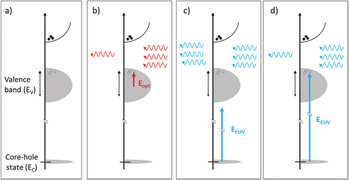
However, EUV photons can become sensitive to valence band excitation if $E_{EUV}$ matches the energy of a core-hole resonance ($E_C$), as sketched in Figure 16 d). In this case EUV photons can be absorbed through a core-valence transition and the spatial modulation of valence band excitations imposed by the EUV TG can produce a diffracted signal with a substantial amplitude, according to Equation 6(6) ${\eta }_F\left(\mathrm{\Delta }t\right)=\frac{I_{sig}}{I_{probe}}={\left|\mathrm{\Delta }n\left({\lambda }_{probe};\mathrm{\Delta }t\right)\right|}^{2}F\left({\lambda }_i,{\theta }_i,L_i,d\right)\xi \left({\sigma }_i,\mathrm{\Delta }{t}_{pump}\right),$(6) -Equation 7(7) $\begin{array}{ll}F\left({\lambda }_i,{\theta }_i,L_i,d\right)=& \frac{cos{\theta }_{sig}}{cos{\theta }_{probe}}{\left[\pi n\left({\lambda }_{probe}\right)d/{\lambda }_{probe}cos\left({\theta }_{probe}\right)\right]}^2\\ & \times \frac{e^{-\left(d/2L^{\ast }\right)}-2cos\left(\mathrm{\Delta }{K}_{z}d\right)e^{-\left(d/2L^{\ast }\right)}+1}{{\left(d/2L^{\ast }\right)}^2+{\left(\mathrm{\Delta }{K}_{z}d\right)}^2}{e}^{-d/L_{abs,probe}cos{\theta }_{sig}},\end{array}$(7) and Equation 13(13) $\mathrm{\Delta }n\left(\lambda \right)=\frac{\partial n}{\partial \rho }\mathrm{\Delta }\rho +{\sum }_s\frac{\partial n}{\partial {\omega }_s}\mathrm{\Delta }{\omega }_s+{\sum }_s\frac{\partial n}{\partial {\gamma }_s}\mathrm{\Delta }{\gamma }_s+\sum _s\frac{\partial n}{\partial g_s}\mathrm{\Delta }{g}_s$(13) -17(17) ${\sum }_s\frac{\partial n\left(\lambda \right)}{\partial g_s}\mathrm{\Delta }{g}_s=\mathrm{\Delta }{n}_g\left(\lambda \right)={\sum }_s\frac{{\omega }^2}{{\omega }^2-{\omega }_s^2+i{\gamma }_s\omega }\mathrm{\Delta }{g}_s$(17) .

On experimental grounds, the weak sensitivity to electronic populations is evident from the data shown in Figure 17 a). Here an EUV TG with $L_{TG}=110$ nm was generated on a 100 nm thick crystalline Si sample and the response was read by using an EUV probe with ${\lambda }_{probe}=17.8$ nm [6], corresponding to the situation sketched in Figure 16 c) since $E_{EUV}=2\pi \hslash c/{\lambda }_{probe}\approx 70$eV is far from the L-absorption edge of silicon ($E_C\approx 100$ eV). The signal is dominated by the dynamics of the density grating, consisting in a slow thermal decay modulated by LA phonon propagation, while for $\mathrm{\Delta }t⩽{\tau }_{e-l}\approx$ 100s of fs there is a much weaker signal on top of the rising signal of the first phonon oscillation (see inset of Figure 17 a); this weak signal is most likely due to the residual sensitivity of the EUV probe to electronic/hole populations in the conduction/valence bands.

Figure 17. a) Black dots connected by lines represent the EUV TG signal with (non-resonant) EUV probe from a silicon sample; this is the first EUV TG waveform ever collected at sub-optical values of ${\text{L}}_{\text{TG}}$ (110 nm in this case). The red line is the slow signal decay, which can be associated with the decay of the thermal grating. The inset is the signal close to time zero sampled with finer steps in $\mathrm{\Delta }t$. The step-like feature is most likely the weak electronic response. b) Comparison of the EUV TG signal with optical (blue line) and EUV probe (black dots connected by lines) from a Si₃N₄ sample. The former data are scaled to fit the same vertical scale while the red dashed line indicates $\mathrm{\Delta }\text{t,}=0$. Despite the ultrafast electronic population grating being similar in both cases, its signal has a much stronger effect when it is “read” by the optical pulse, leading to a maximum signal intensity at $\mathrm{\Delta }\text{t,}=\text{,}0$, while it results in a faint “bump” at $\mathrm{\Delta }\text{t,}=\text{,}0$ when EUV probing is employed. The maximum EUV TG signal intensity with EUV probing is not reached at $\mathrm{\Delta }\text{t,}=\text{,}0$ but at half of the LA period (${\text{t}}_{\text{LA}}/2$), indicated by the yellow arrow. Note that the values of ${\text{L}}_{\text{TG}}$ were different in these two cases, i.e. ${\text{L}}_{\text{TG}}$ = 85/280 nm for EUV/optical probing, but this is not relevant when ${\text{L}}_{\text{TG}}>{\text{L}}_{\text{e}}$, as in the present case. Figure adapted from [6].

The phonon modulation frequency was found to be compatible with the one expected for longitudinal acoustic phonons, ${\omega }_{LA}=2\pi c_{LA}/L_{TG}$, while the thermal decay was found to be one order of magnitude slower than what expected from Fourer law of diffusion [6]. Deviations with respect to the diffusive behaviour in crystalline silicon were actually observed by optical TG already at µm length-scales [5,239]. In order to understand this large discrepancy with respect to the diffusive regime further EUV TG data with higher quality and at different values of $L_{TG}$ have been collected and interpreted within a proper nanoscale thermal transport model [240]. Figure 17 b) displays a comparison between optical (${\lambda }_{probe}=390$ nm) and non-resonant EUV probe (${\lambda }_{probe}=13.3$ nm) on the same sample (100-nm thick Si₃N₄) [6]. In the first case the time resolution was about 160 fs, limited by the time duration and incidence angle of the optical probe, while in the latter was about 60 fs, limited by the FEL time duration. As expected from the above reasoning, the optical probe is strongly affected by spatially modulated valence excitations, resulting in a bright transient diffraction signal at time-zero with a fast (resolution limited) rise time and a 100s fs decay, as explained in section 3.3.1. We finally notice that the value of $L_{TG}$ was different for the two datasets shown in Figure 17 b), i.e. 270 nm (optical probe) vs 85 nm (EUV probe). This is irrelevant for the electronic dynamics stimulated by EUV pulses, as long as $L_{TG}>L_e$ (see Figure 8). One can therefore assume the same excitation mechanism in both cases and the substantial and qualitative differences between the two signals can be fully ascribed by the different couplings between the probe and the excited sample.

In Figure 18 we compare EUV TG data from the same sample (a 40 nm thick Co film deposited on a 50 nm thick Si₃N₄ membrane) collected with a non-resonant (${\lambda }_{probe}=13.3$ nm) and a resonant EUV probe (${\lambda }_{probe}=20.8$ nm); in the latter case the probed resonance was the Co M-edge. For non-resonant EUV probe (Figure 18 a) the signal is qualitatively similar to the one shown in Figure 17 a), i.e. a thermal decay modulated by LA phonons at the expected frequency ${\omega }_{LA}=2\pi c_{LA}/L_{TG}=$ 0.54 THz (where $c_{LA}$ = 10.4 km/s and $L_{TG}$ was 16.7 nm). It is interesting to notice how, for this value of $L_{TG}$, the thermal decay time is actually on the same order as $t_{LA}$, meaning that the $k_{exc}$-dependencies of ${{\tau }_T}^{-1}$ and ${\omega }_{LA}$ (see Figure 1) bring these two quantities to the same value at such length-scale. On the other hand, the EUV resonant probe (Figure 18, panel b) displays a large time zero signal, similar to the one observed with the optical probe from all the samples studied so far, i.e. a fast (resolution limited at $\approx 50$fs) rise time and a 100s fs decay (see sections 3.3.2–3.3.4). The shape of the non-resonant and resonant signal waveforms in the first ps range is shown, respectively, in the insets of Figure 18 a) and b). Data in Figure 18 b) have been collected at $L_{TG}=$ 44 nm, however, as explained above, the value of $L_{TG}$ changes the thermal decay time and modulation frequency in the thermoelastic waveform, but it is not relevant to the purpose of comparing the ultrafast electronic response.

Figure 18. a) EUV TG signal from a 40 nm thick Co at ${\text{L}}_{\text{TG}}$ = 16.7 nm collected with a non-resonant EUV probe (${\lambda }_{\text{probe}}$ = 13.3 nm). The waveform is consistent with a thermal decay modulated by phonon oscillations and no sizable signal at $\mathrm{\Delta }\text{t,}=0$ is observed (see inset for an enlargement of the time zero region). This value of ${\text{L}}_{\text{TG}}$ is the shortest achieved so far with EUV TG. b) EUV TG signal from a 40 nm thick Co at ${\text{L}}_{\text{TG}}$ = 44 nm collected with an EUV probe resonant with the M-edge of cobalt (${\lambda }_{\text{probe}}$ = 20.8 nm). A prominent electronic signal is observed, like in optically probed EUV TG (see e.g. Figure 9 a). Blue and red lines are, respectively, a gaussian function with 60 fs FWHM, compatible with the time resolution of the experiment, and an exponential decay with 250 fs time constant, compatible with typical electron-lattice relaxation times. The thermoelastic signal at longer $\mathrm{\Delta }\text{t}$ is weakly visible in this vertical scale. Panel b) is adapted from [118].

Figure 18a) also illustrates another advantage of EUV over optical probes for TG experiments in forward diffraction: the possibility to probe bulk metallic samples. In fact, optical photons typically have photon energies below the plasma frequency of metals and, consequently, are simply not transmitted by the sample. The study of metals using optical probes is hence typically restricted to the surface response. More generally, EUV probes are an optimal choice for probing thermoelastic dynamics, since refractive index variations due to density changes are in most cases the dominant contribution to the EUV TG signal. On the other hand, EUV probes only couple weakly with $\mathrm{\Delta }{n}_R\left({\lambda }_{probe};\mathrm{\Delta }t\right)$, thus preventing from the observation of Raman modes. This is because the changes in the molecular polarizability due to DECP mechanism marginally affect EUV photons with E_EUV largely exceeding the typical values of $\hslash {\omega }_R$ (see Equation 10(10) $\mathrm{\Delta }{n}_{Raman}\left({\lambda }_{probe};\mathrm{\Delta }t\right)/n=A{e}^{-\beta \mathrm{\Delta }t}+B{e}^{-\gamma \mathrm{\Delta }t}\left(cos\left(\mathrm{\Omega \Delta }t\right)-\frac{\beta -\gamma }{\mathrm{\Omega }}sin\left(\mathrm{\Omega \Delta }t\right)\right),$(10) ). As a matter of fact, we never observed Raman oscillations by using EUV probes. However, Raman modes induce a dynamic variation of the bond length, which may be a substantial fraction ($\approx$ 1%) of the bond length at rest. This may affect the values of the parameters of core-hole resonances, therefore molecular vibrations may be observable in EUV TG with resonant EUV probes. Though we do not have any corroborating experimental evidence yet, it is worth mentioning that molecular vibrations are observable in optical-pump/X-ray-probe experiments [241,242]. Such approaches provide the unique possibility to add elemental selectivity to vibrational dynamics studies, with the additional capabilities of correlating vibrational and electronic dynamics [243] and to add enantiomeric selectivity [244]. In this context, EUV TG would add the $k_{exc}$variable and the capability to access the nanoscale.

We finally mention that data shown in Figure 17 are the first EUV TG data with EUV probe ever collected and correspond to the most favourable experimental geometry, while those in Figure 18 a), (previously unpublished) have been acquired more recently and are those obtained with the shortest value of $L_{TG}$ exploited so far, i.e. with the most unfavourable experimental conditions considered up to now. In both cases the acquisition time was a couple of hours, indicating how the general quality of the data improved in these few years of operation of the instrument.

3.5.3 EUV probing: forward vs backward diffraction

Analogously to the discussion made above about the comparison between optical and EUV probe in the case of forward diffraction, EUV probing of refractive index modulations at the surface due to electronic excitations, $\mathrm{\Delta }{n}_{surf}^2\left({\lambda }_{probe};\mathrm{\Delta }t\right)$, may result into a large ultrafast EUV TG signal only when ${\lambda }_{probe}$ matches an electronic core resonance. Conversely, for optical probes the magnitude of $\mathrm{\Delta }{n}_{surf}^2\left({\lambda }_{probe};\mathrm{\Delta }t\right)$ typically results in a large signal, like the data shown in Figure 11a). However, to date we do not have EUV TG data with resonant EUV probing in backward diffraction geometry to experimentally corroborate this expectation.

On the other hand, EUV probes in backward diffraction are sensitive to coherent surface displacements as long as the EUV reflectivity is not zero, see Equation 9(9) $\begin{array}{ll}{\eta }_B\left(\mathrm{\Delta }t\right)=& \left[R{\left(2\frac{\pi u_z\left(\mathrm{\Delta }t\right)}{{\lambda }_{probe}}\right)}^{2}cos\left({\theta }_{sig}\right)cos\left({\theta }_{probe}\right)+\mathrm{\Delta }{n}_{surf}^2\left({\lambda }_{probe};\mathrm{\Delta }t\right)/4\right]\\ & \times \xi \left({\sigma }_i,\mathrm{\Delta }{t}_p\right),\end{array}$(9) This permits to collect, in a relatively easy way, EUV TG waveforms in backward diffraction at $L_{TG}<$ 100 nm and to gain information on high frequency SAWs and thermal relaxations. Figure 19a) reports the first EUV TG data (previously unpublished) with EUV probing in backward diffraction (${\lambda }_{probe}=$ 13.3 nm). The sample was a 100 nm thick film of a PdSiCu metallic glass deposited on a bulk SiO2 substrate. The overall sample (film plus substrate) is not transparent to the EUV radiation, but this is not a requirement in this case since the signal is collected in reflection. The amplitude of the thermoelastic signal is larger than the ones shown in Figures 17 and 18; for data in Figures 17 and 18 we used the same normalization procedure as in Figure 19a. In many other cases we observed backward diffracted EUV TG signals with intensity similar or larger than what is observed in forward diffraction in similar samples [118]. Large backward diffracted signals are not unexpected, since depending on specific sample parameters and experimental geometry the value of ${\eta }_B$ (Equation 9(9) $\begin{array}{ll}{\eta }_B\left(\mathrm{\Delta }t\right)=& \left[R{\left(2\frac{\pi u_z\left(\mathrm{\Delta }t\right)}{{\lambda }_{probe}}\right)}^{2}cos\left({\theta }_{sig}\right)cos\left({\theta }_{probe}\right)+\mathrm{\Delta }{n}_{surf}^2\left({\lambda }_{probe};\mathrm{\Delta }t\right)/4\right]\\ & \times \xi \left({\sigma }_i,\mathrm{\Delta }{t}_p\right),\end{array}$(9) ) may be larger than ${\eta }_F$ (Equation 6(6) ${\eta }_F\left(\mathrm{\Delta }t\right)=\frac{I_{sig}}{I_{probe}}={\left|\mathrm{\Delta }n\left({\lambda }_{probe};\mathrm{\Delta }t\right)\right|}^{2}F\left({\lambda }_i,{\theta }_i,L_i,d\right)\xi \left({\sigma }_i,\mathrm{\Delta }{t}_{pump}\right),$(6) -Equation 7(7) $\begin{array}{ll}F\left({\lambda }_i,{\theta }_i,L_i,d\right)=& \frac{cos{\theta }_{sig}}{cos{\theta }_{probe}}{\left[\pi n\left({\lambda }_{probe}\right)d/{\lambda }_{probe}cos\left({\theta }_{probe}\right)\right]}^2\\ & \times \frac{e^{-\left(d/2L^{\ast }\right)}-2cos\left(\mathrm{\Delta }{K}_{z}d\right)e^{-\left(d/2L^{\ast }\right)}+1}{{\left(d/2L^{\ast }\right)}^2+{\left(\mathrm{\Delta }{K}_{z}d\right)}^2}{e}^{-d/L_{abs,probe}cos{\theta }_{sig}},\end{array}$(7) , even from samples with an optimal thickness [118]. Figure 19b displays a few examples of the expected values of ${\eta }_B$ and ${\eta }_F$, computed by using tabulated data [245], assuming an angle of incidence of 80°, $\mathrm{\Delta }{K}_z=0$ and ${\lambda }_{pump}={\lambda }_{probe}$ in Equation 6(6) ${\eta }_F\left(\mathrm{\Delta }t\right)=\frac{I_{sig}}{I_{probe}}={\left|\mathrm{\Delta }n\left({\lambda }_{probe};\mathrm{\Delta }t\right)\right|}^{2}F\left({\lambda }_i,{\theta }_i,L_i,d\right)\xi \left({\sigma }_i,\mathrm{\Delta }{t}_{pump}\right),$(6) -Equation 7(7) $\begin{array}{ll}F\left({\lambda }_i,{\theta }_i,L_i,d\right)=& \frac{cos{\theta }_{sig}}{cos{\theta }_{probe}}{\left[\pi n\left({\lambda }_{probe}\right)d/{\lambda }_{probe}cos\left({\theta }_{probe}\right)\right]}^2\\ & \times \frac{e^{-\left(d/2L^{\ast }\right)}-2cos\left(\mathrm{\Delta }{K}_{z}d\right)e^{-\left(d/2L^{\ast }\right)}+1}{{\left(d/2L^{\ast }\right)}^2+{\left(\mathrm{\Delta }{K}_{z}d\right)}^2}{e}^{-d/L_{abs,probe}cos{\theta }_{sig}},\end{array}$(7) , an amplitude of the lattice temperature grating of 100 K and a thermal expansion coefficient $\alpha =$10⁻⁵ K⁻¹. These are strong assumptions but are sufficiently reasonable for illustrative purposes. A critical requirement for EUV TG in backward diffraction is the surface quality, since a surface roughness already at the nm level may be detrimental for the EUV reflectivity and thus for ${\eta }_B$, as shown in Figure 19b for the case of carbon. The initial rise time of the waveform in Figure 19a is not perfectly sinusoidal, and may indicate a faster modulation. This behaviour was observed in many samples and might be related to LA modes launched in the direction perpendicular to the surface, as explained in Section 3.3.3 in the case of EUV TG with optical probing. Further investigations to corroborate this hypothesis are ongoing.

Figure 19. a) EUV TG signal with EUV probing collected in backward diffraction from a 100 nm thick PdSiCu sample on a SiO₂ bulk substrate. The inset shows the initial rise of the signal, the red line is a sinusoidal profile. b) Estimated trend of forward diffraction efficiency (${\eta }_{\text{F}}$) for carbon (full black lines), silicon (full red line) and terbium (full blue lines) for an optimal sample length as a function of wavelength ($\lambda$) on going from the EUV to the hard X-ray regime; see text for further details. Dashed and dot-dashed red lines are the trend of backward diffraction efficiency (${\eta }_{\text{B}}$) for silicon by assuming, respectively, a root-mean-square value of the surface roughness of 0.1 and 1 nm; in both cases a 20° grazing angle for the probe was considered. Data are plotted in a double logarithmic scale with reversed horizontal axis. On moving from the EUV to the hard X-ray range ${\eta }_{\text{F}}$ becomes increasingly more favourable.

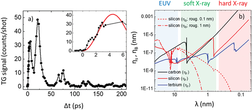
The high absorption and low reflectivity of EUV light as compared with optical precludes the observation of the ‘spurious mixing’ between backward and forward diffraction due to the reflection of the optical probe from the back surface of an optically transparent sample, as explained in section 3.3.3 [218]. However, as explained above, it is possible to detect the dynamics of surface displacement in forward diffraction, since the spatially periodic surface displacement (and also thickness variations in thin samples) can produce diffraction in forward direction, and it is also possible to detect the effects of bulk modes, such as SSLW, in backward diffraction.

EUV TG at sub-100 nm wavelength in forward diffraction requires the use of sufficiently thin samples to enable a tangible transmission of the probe beam (see Equation 7(7) $\begin{array}{ll}F\left({\lambda }_i,{\theta }_i,L_i,d\right)=& \frac{cos{\theta }_{sig}}{cos{\theta }_{probe}}{\left[\pi n\left({\lambda }_{probe}\right)d/{\lambda }_{probe}cos\left({\theta }_{probe}\right)\right]}^2\\ & \times \frac{e^{-\left(d/2L^{\ast }\right)}-2cos\left(\mathrm{\Delta }{K}_{z}d\right)e^{-\left(d/2L^{\ast }\right)}+1}{{\left(d/2L^{\ast }\right)}^2+{\left(\mathrm{\Delta }{K}_{z}d\right)}^2}{e}^{-d/L_{abs,probe}cos{\theta }_{sig}},\end{array}$(7) ), which typically means thicknesses of 10s to 100s of nm. This is a relevant constraint, since not all samples can be fabricated as sub-um membranes. Thin films on bulk supports do not work as well, since the support should transmit the probe beam and there are no materials that transmit EUV light for several μm. Backward diffraction can be used on a larger variety of samples, since it permits to remove the strict requirement of the sample thickness while adding the one of a smooth surfaces, which is much easier to meet.

Neutron and X-ray spectroscopy, as well as FT-IXS, are not sensitive to surfaces. X-rays at grazing incidence can be used to probe optically excited surface modes [155], but these are limited to optical wavelengths. Therefore the $\left({\omega }_{exc},k_{exc}\right)$-range accessible by the various techniques shown in Figure 1 lacks all short-wavelength probes, making EUV TG with EUV probe in backward diffraction the only ‘contactless’ method to probe surface phonons at sub-100 nm wavelength, and potentially also surface electronic dynamics via resonant EUV probing. Most likely this uniqueness will be retained also after the envisionable extension of EUV TG towards the X-ray regime, with TG both generated and probed by X-ray pulses. In fact, the large decrease in reflectivity at X-ray wavelengths and the stronger detrimental effect of surface roughness (see Figure 19 b) will probably make X-ray TG in backward diffraction unfeasible, unless envisioning an unpractical grazing incidence geometry (the ${\eta }_B$ vs $\lambda$ curves in Figure 19 b correspond to 20° grazing angle), which might also be highly demanding in terms of X-ray pump intensity at sample (because of the likely large footprint of the pump). On the other hand, the longer penetration depth of X-ray light is expected to have two relevant benefits in forward diffraction: to remove the necessity of thin samples and to provide a much stronger signal (see Figure 19 b), which is essentially due to the possibility of using thicker samples because of the d² dependence in Equation 7(7) $\begin{array}{ll}F\left({\lambda }_i,{\theta }_i,L_i,d\right)=& \frac{cos{\theta }_{sig}}{cos{\theta }_{probe}}{\left[\pi n\left({\lambda }_{probe}\right)d/{\lambda }_{probe}cos\left({\theta }_{probe}\right)\right]}^2\\ & \times \frac{e^{-\left(d/2L^{\ast }\right)}-2cos\left(\mathrm{\Delta }{K}_{z}d\right)e^{-\left(d/2L^{\ast }\right)}+1}{{\left(d/2L^{\ast }\right)}^2+{\left(\mathrm{\Delta }{K}_{z}d\right)}^2}{e}^{-d/L_{abs,probe}cos{\theta }_{sig}},\end{array}$(7) The trend of ${\eta }_F$ shown in Figure 19 b) assumes a given amplitude of the lattice temperature grating ($\mathrm{\Delta }T=$ 100 K in this case) that is in the estimated range for typical EUV TG experiments. However, since $L_{abs}$ substantially increases towards the X-ray range, the X-ray fluence needed to reach the same value of $\mathrm{\Delta }T$ should increase correspondingly. Most likely, in realistic conditions X-ray TG experiments in forward diffraction would not show an increase in efficiency as large as the one displayed in Figure 19 b).

3.5.4 Magnetic dynamics through resonant EUV probing

Among the electronic related phenomena that can be observed with TG, magnetism is of particular relevance. Studying magnetic properties at the nanoscale is an open and appealing topic with fallouts in various technological fields ranging from efficient computation techniques to data storage. In a uniformly magnetised sample, EUV TG can cause periodic demagnetization due to the electronic temperature increase that ultimately turns into a periodic arrangement of the refractive index, as schematized in Figure 20 a). In magnetic materials, the complex refractive index depends on both magnetization and the polarisation of light [246]: Equation 18(18) $n_{\pm }=1-\left(\delta \pm \mathrm{\Delta }\delta \right)+i\left(\beta \pm \mathrm{\Delta }\beta \right),$(18)

Figure 20. a) Sketch of the experiment: at $\mathrm{\Delta }\text{t}<0$ the CoGd sample is uniformly magnetized (aligned orange arrows) by a saturating magnetic field (H). At $\mathrm{\Delta }\text{t}=0$ it is excited by the nanoscale EUV TG (${\text{L}}_{\text{TG}}$= 44 nm), the thermal grating drives ultrafast demagnetization (disordered orange arrows) in the constructive interference (hot) regions. For $\mathrm{\Delta }\text{t,}⩾\text{,}0$ the probe beam (red arrow) resonant with the Co M-edge (${\lambda }_{\text{probe}}\text{,}=$ 20.8 nm) and linearly polarized (orthogonally to the plane is diffracted by the spatially modulated magnetization via the refractive index variation (see Equation 19(19) $\mathrm{\Delta }{n}_{CR,CL}\left({\lambda }_{probe};x,\mathrm{\Delta }t\right)=\pm \left(\mathrm{\Delta }\delta \left({\lambda }_{probe}\right)+i\mathrm{\Delta }\beta \left({\lambda }_{probe}\right)\right)\frac{\mathrm{\Delta }M\left(\mathrm{\Delta }t\right)}{M_0}cos\left(k_{TG}x\right)$(19) ), generating a signal beam with in-plane linear polarization. At longer time scales ($\mathrm{\Delta }\text{t}\to \mathrm{\infty }$) the initial magnetic state is restored by H. b) Black circles connected by lines are the EUV TG signal due to magnetization dynamics, collected with the saturating magnetic field ON. The waveform is strongly non-sinusoidal, with $\approx$ 1 ps rise time and a 10 ps decay. Red points connected by lines are the EUV TG signal collected with the H=0 (saturating magnetic field OFF). In this case the magnetic signal averages to zero and the electronic signal at $\mathrm{\Delta }\text{t}=$ 0 is clearly visible, as well as a weaker signal at $\mathrm{\Delta }\text{t}>$ 0, likely due to the thermoelastic response. Figure adapted from [217].

(18) $n_{\pm }=1-\left(\delta \pm \mathrm{\Delta }\delta \right)+i\left(\beta \pm \mathrm{\Delta }\beta \right),$(18)

where the subfix $\pm$ corresponds, respectively, to the parallel and antiparallel orientation of the photon helicity with respect to the sample magnetization, while $\mathrm{\Delta }\delta$ and $\mathrm{\Delta }\beta$ are the magneto-optical constants. The spatial variation of magnetization induced by the thermal grating hence reflects in a sinusoidal variation of the refractive index that can be written as: Equation 19(19) $\mathrm{\Delta }{n}_{CR,CL}\left({\lambda }_{probe};x,\mathrm{\Delta }t\right)=\pm \left(\mathrm{\Delta }\delta \left({\lambda }_{probe}\right)+i\mathrm{\Delta }\beta \left({\lambda }_{probe}\right)\right)\frac{\mathrm{\Delta }M\left(\mathrm{\Delta }t\right)}{M_0}cos\left(k_{TG}x\right)$(19)

(19) $\mathrm{\Delta }{n}_{CR,CL}\left({\lambda }_{probe};x,\mathrm{\Delta }t\right)=\pm \left(\mathrm{\Delta }\delta \left({\lambda }_{probe}\right)+i\mathrm{\Delta }\beta \left({\lambda }_{probe}\right)\right)\frac{\mathrm{\Delta }M\left(\mathrm{\Delta }t\right)}{M_0}cos\left(k_{TG}x\right)$(19)

where $\mathrm{\Delta }M\left(t\right)/M_0$ is the relative variation of the magnetization and the subfix $CR/CL$ stands for circular right and circular left polarisation of the probing light. A linearly polarised pulse can be decomposed into a superposition of CR and CL polarised beams, and effectively sees simultaneously two gratings that diffract the two components differently. The unbalance between the diffraction of CL and CR components leads to a 90° rotation of the polarisation of the signal beam with respect to that of the probe beam [217], see Figure 20 a). Since thermoelastic and electronic signals are not expected to rotate the polarisation, the EUV TG signal of magnetic nature can be isolated through a polarization analysis of the signal beam.

Figure 20 illustrates the EUV TG experiment when the first magnetic signal was observed [217]. The sample was a 9 nm thick ferrimagnetic film of Co_0.81Gd_0.19 alloy on a 100 nm thick Si₃N₄ membrane, showing perpendicular magnetic anisotropy and placed in a saturating out-of-plane magnetic field (H) in order to force a spatially uniform magnetization state before the interaction with the pump pulses; see panel a). The value of ${\lambda }_{probe}$ was tuned to 20.8 nm in order to match the cobalt M-edge; data shown in Figure 20 b) was obtained by setting ${\lambda }_{pump}={\lambda }_{probe}$ and $2\theta =$ 27.6°, corresponding to $L_{TG}\approx$ 44 nm. The EUV TG signal waveform (black dataset) is non-sinusoidal, with $\approx$ 1 ps rise time and $\approx$ 10 ps decay, and no oscillations typical of the thermoelastic response (see Figures 17–19) can be perceived. Red points connected by lines indicate the EUV TG signal collected with H = 0; in this case the magnetic signal averages to zero, since the magnetic domains that are naturally present in the sample have sizes comparable to $L_{TG}$. In this condition the electronic signal at $\mathrm{\Delta }t=$ 0 is clearly visible, as expected in the case of resonant EUV probing, while the weaker signal at $\mathrm{\Delta }t>$ 0 is likely due to the thermoelastic response. This result demonstrates the possibility to generate nanoscale modulations of magnetization and probe their time dependence with ultrafast time resolution. Furthermore, these initial results show how the amplitude of the magnetic EUV TG signal can be larger than the one associated with the thermoelastic response. We observe that Equation 19(19) $\mathrm{\Delta }{n}_{CR,CL}\left({\lambda }_{probe};x,\mathrm{\Delta }t\right)=\pm \left(\mathrm{\Delta }\delta \left({\lambda }_{probe}\right)+i\mathrm{\Delta }\beta \left({\lambda }_{probe}\right)\right)\frac{\mathrm{\Delta }M\left(\mathrm{\Delta }t\right)}{M_0}cos\left(k_{TG}x\right)$(19) has the same structure as Equation 14(14) $\frac{\partial n\left(\lambda \right)}{\partial \rho }\mathrm{\Delta }\rho =\mathrm{\Delta }{n}_{\rho }\left(\lambda \right)=\left(\frac{r_e{\lambda }^2}{2\pi }f{}^{\prime }\left(\omega \right)+\frac{i{r}_e{\lambda }^2}{2\pi }f{}^{\prime \prime }\left(\omega \right)\right)\mathrm{\Delta }\rho =\left(\delta +i\beta \right)\frac{\mathrm{\Delta }\rho }{\rho }$(14) , where $\delta$ and $\beta$ are replaced by $\mathrm{\Delta }\delta$ and $\mathrm{\Delta }\beta$ and $\mathrm{\Delta }\rho /\rho$ is replaced by $\mathrm{\Delta }M/M$. While the value of $\mathrm{\Delta }\delta$ and $\mathrm{\Delta }\beta$ can be on the same order as $\delta$ and $\beta$, the value of $\mathrm{\Delta }M/M$ can be in the few % to several 10s % with moderate EUV excitation fluences, comparable with those used to collect the thermoelastic signals reported in Figures 17–19. For the same excitation fluence the values of $\mathrm{\Delta }\rho /\rho$ are instead in the 0.1% range (assuming $\mathrm{\Delta }T\approx 100$ K and $\alpha \approx$ 10⁻⁵ K⁻¹) or even lower. Recalling that the EUV TG signal is quadratic in the refractive index variation, the ratio between the magnetic and the thermoelastic response in the EUV TG signal can easily exceed a factor 10.

Similarly to the thermoelastic case, EUV TG excitation is expected to launch propagating spin waves, or magnons, at a given $k_{exc}=k_{TG}$. The coherent excitation of magnons was not yet observed since, in all experiments performed to date, H was aligned parallel to the perpendicular magnetic anisotropy of the investigated ferrimagnetic alloys; in this configuration, thermal excitation by either optical or EUV pulses does not initiate the precession of the magnetization. To excite a coherent magnon in a ferromagnet via thermal mechanism one needs a tilted external magnetic field as was shown in optical pump-probe experiments, where magnons at $k_{exc}\approx$ 0 were detected. Optical TG was also used to excite spin waves at optical wavevectors, whose dynamics were probed in a very effective way and in real-space by ultrafast Lorentz transmission electron microscopy [216].

Additional magnetic length scales that can match the spatial periodicity of EUV TG are the exchange coupling and spin diffusion length scales, as well as the intrinsic dimension of magnetic domains. Therefore, ultrafast experiments as a function of $L_{TG}$ in the sub-100 nm range may reveal fundamental details of magnetic processes. Finally, it is worth mentioning that, while transient magnetization gratings with periodicity in the 100s of nm range have been excited with optical light by permanently nanostructuring the sample with near field masks [247], EUV TG excitation provides a unique and contactless mean of controlling magnetic properties.

4 Showcase of sub-100 nm TG examples

In the previous section we illustrated the dynamics that can be determined in EUV TG experiments with both optical and EUV probes, showing the first measurements carried out with values of $L_{TG}$ in the sub-100 nm range. Further below we discuss other examples of applications of EUV TG at the sub-100 nm scale.

4.1 Thermoelastic response vs phonon wavelength

In Figure 21 a) we show the first EUV TG dataset collected as a function of $k_{TG}$ [6]. The sample was a 100 nm thick amorphous Si₃N₄ membrane and the value of $k_{TG}$ was changed by changing ${\lambda }_{pump}$ (53.4, 39.9 and 13.3 nm) while keeping the value of $\theta$ fixed. ${\lambda }_{probe}$ was also kept fixed at 13.3 nm, a value far from any core hole resonance in the sample. The signal waveforms are qualitatively similar to the ones shown in Figures 17 and 18, consisting in a slow thermal decay with modulations due LA phonons, as expected from non-resonant EUV probing. The values of ${\tau }_{th}$ and ${\omega }_{LA}$ were respectively extracted from the waveforms by exponential fits (red lines in Figure 21 a) and Fourier transforms. These indicate other minor frequency contents besides ${\omega }_{LA}$, as also evident by the beatings visible in the waveforms. However, the quality of these data was not sufficient to carry out a proper analysis and we initially neglected these additional frequencies. Nevertheless,, as will be discussed in detail in the next section, multiple frequencies related to different vibrational modes of the Si₃N₄ membrane are actually expected since the thickness of the sample is comparable to $L_{TG}$. Figure 21 b) and c) show, respectively, ${{\tau }^{-1}}_{th}$ and ${\omega }_{LA}$ as a function of $k_{TG}$, showing a linear trend for ${\omega }_{LA}$ and a quadratic one for ${{\tau }^{-1}}_{th}$. The latter indicates a diffusive transport and is expected in amorphous solids at this still relatively long length-scales. The coefficient of the linear dispersion of ${\omega }_{LA}$vs $k_{TG}$ matches well the expected value of the LA sound velocity ($c_{LA}=$ 10.4 km/s).

Figure 21. Black dots connected by lines in panels a), b) and c) are the EUV TG signal from a 100 nm thick SiN sample collected, respectively, at110, 85 and 28 nm. The red lines indicate the slow signal decay. Panel d) and e) report, respectively, the angular frequency of the oscillations (${\omega }_{L}A$) and the decay rate of the signal $({{\tau }^{-1}}_T)$ as a function of. Blue lines in Panels d) and e) are, respectively, quadratic and linear trends with coefficients cLA = 10.4 km/s and DT = 1.05 nm2/ps. Figure adapted from [6].

These results demonstrated stimulated Brillouin scattering of EUV light, using a time domain methodology to overcome the limitations imposed by the finite energy resolution of EUV spectrometers, the capability to detect phonon modes in the 10s of nm wavelength range, previously inaccessible, and nanoscale heat transport dynamics without the need to modify or contact the specimen.

4.2 Thermoelasticity in confined systems

In order to analyse the EUV TG signal dependencies on the finite dimension of samples, which is relevant when studying membranes and coatings with thickness comparable to $L_{TG}$, higher quality EUV TG data in forward diffraction from Si₃N₄ membranes were collected more recently for different values of both $L_{TG}$ and membrane thickness (d) [248]. Examples of experimental waveforms are shown in Figure 22 a) and c). In both cases d = 100 nm while $L_{TG}$ was 84 nm (Panel a) and 44 nm (Panel c), obtained by changing ${\lambda }_{pump}$ from 39.9 nm to 20.8 nm at fixed $2\theta =$27.6°; ${\lambda }_{probe}$ was also changed from 13.3 nm to 20.8 nm. The change in ${\lambda }_{pump}$ implied a change in $L_{abs,pump}$, which resulted in a different amplitude of the lattice temperature grating and thus in a different sample heating due to the FEL pump. One can readily appreciate a prominent beating at $L_{TG}=$84 nm while on reducing $L_{TG}$ to 44 nm the waveform becomes more similar to a simple sinusoidal oscillation. This is also evident from the Fourier transforms reported in the insets.

Figure 22. Black dots connected by lines in panels a) and b) are the EUV TG signal from Si3N4 collected, respectively, at ${\text{k}}_{\text{exc}}\text{d}\approx$ 7.5 and 14. The red lines are best fits of the data using Equation 20(20) $I_{TG}={\left|A_T{e}^{-\mathrm{\Delta }t/{\tau }_T}+{\mathrm{\Sigma }}_i{A}_{i}cos\left({\omega }_i\mathrm{\Delta }t\right)e^{-\mathrm{\Delta }t/{\tau }_i}\right|}^2,$(20) , while insets show the Fourier transform of the experimental waveform. Panels c) and b) are the dispersion relations calculated from Lamb wave theory (only symmetric modes are considered), the blue circles are the frequencies extracted from the fit while the straight red line is the LA frequency; for a given value of ${\text{k}}_{\text{exc}}$ the brightest Lamb modes in the EUV TG signal are those closer to such frequency. Figure adapted from [248].

In the usual treatment of elastic fields in solid media, the stress-free boundary condition is set at infinity. In the case of membranes, this does not hold anymore and stress-free conditions happen at the surfaces which are separated by the membrane thickness ‘d’. The finite system then supports a greater number of modes that can be classified as symmetric or antisymmetric depending on the geometry of the deformation with respect to the sample median plane [136]. These waves, usually referred to as Lamb waves, are a combination of the usual transverse acoustic (TA) and LA modes that can be detected in thick solids and their dispersion relations can be expressed as a function of $k_{exc}d$, i.e. the product of their wavevector and the sample thickness. Exemplificative dispersion curves are shown in Figure 23 b) to d). At large values of $k_{exc}d$ the system recovers the bulk behaviour (this is usually assumed to occur for $k_{exc}d>$ 10), with all the dispersion curves collapsing in the LA and SAW modes [136,249].

Figure 23. In both main panels we plot the EUV TG data shown in Figure 22a in the time delay range $\mathrm{\Delta }\text{t,}$= 270–520 ps, while insets show the same data for $\mathrm{\Delta }\text{t,}$= −20–320 ps. The red lines are best fits of the data using Equation 20(20) $I_{TG}={\left|A_T{e}^{-\mathrm{\Delta }t/{\tau }_T}+{\mathrm{\Sigma }}_i{A}_{i}cos\left({\omega }_i\mathrm{\Delta }t\right)e^{-\mathrm{\Delta }t/{\tau }_i}\right|}^2,$(20) , by assuming ${\tau }_{\text{ph}}=\mathrm{\infty }$ (Panel a) or letting this parameter free to vary (Panel b). The latter fit describes much better the data for $\mathrm{\Delta }\text{t,}$= 270–520 ps (main panels), while both fits well describe the data for $\mathrm{\Delta }\text{t,}$= 270–520 ps (insets). Figure adapted from [248].

Both the waveforms of panels a) and c) can be explained in terms of interference between Lamb modes and their temporal evolution can be reproduced with the function: Equation 20(20) $I_{TG}={\left|A_T{e}^{-\mathrm{\Delta }t/{\tau }_T}+{\mathrm{\Sigma }}_i{A}_{i}cos\left({\omega }_i\mathrm{\Delta }t\right)e^{-\mathrm{\Delta }t/{\tau }_i}\right|}^2,$(20)

(20) $I_{TG}={\left|A_T{e}^{-\mathrm{\Delta }t/{\tau }_T}+{\mathrm{\Sigma }}_i{A}_{i}cos\left({\omega }_i\mathrm{\Delta }t\right)e^{-\mathrm{\Delta }t/{\tau }_i}\right|}^2,$(20)

where $A_i$, ${\omega }_i$ and ${\tau }_i$ are respectively the amplitude, frequency and decay time of the single Lamb modes.

The fit to the data in Figure 22, with Equation 20(20) $I_{TG}={\left|A_T{e}^{-\mathrm{\Delta }t/{\tau }_T}+{\mathrm{\Sigma }}_i{A}_{i}cos\left({\omega }_i\mathrm{\Delta }t\right)e^{-\mathrm{\Delta }t/{\tau }_i}\right|}^2,$(20) yields two modes with $A_1=1.6$ and 1.7 and ${\omega }_1=$ 0.7 THz and ${\omega }_2=$ 0.78 THz; the similar amplitudes and frequencies give rise to the observed beating pattern. A comparison with the theoretical dispersion curves (Figure 22) reveals that two symmetric modes, both close to the LA frequency, are expected. In this plot we report only symmetric modes, which should provide the most sizable contributions in these experimental conditions. Though contemplated by the calculations, we do not observe additional modes in the waveform since the value of $k_{exc}b$ is already quite large and, therefore, Lamb modes with significant amplitudes are predicted to be the ones closer to LA and SAW frequency (the latter being eventually observable in backward diffraction, not employed in the present experiment). The magnitude of this frequency splitting is essentially related to the effect of TA-LA coupling. Figure 22 shows how for larger values of $k_{exc}d$ (about 14 in this case) the waveform approximates, as expected, a single oscillation. The Fourier transform exhibits a single peak, albeit with a little asymmetry that may hide a weak additional frequency content. A careful fit of the waveform in fact reveals the presence of two modes, close in $\omega$ with $A_1=2$ and $A_2=0.3$. The unbalance of the mode amplitudes generates a less evident beating pattern. Please note that, although calculated for the same sample, the dispersion curves of panel b) are slightly shifted with respect to those in panel d) to take into account different sample temperatures associated with a slight difference in the deposited pump energy. The comparison with the calculated dispersion relation (Figure 22d) displays two modes very close to each other and to the LA frequency. The trend of ${{\tau }_T}^{-1}$ vs $k_{TG}$ is in agreement with the results reported in Figure 21e).

Lamb waves, even though requiring a more complex data analysis, are a valuable tool to extract information about modes not normally visible. For example, LA phonons are expected to be observable in transmission geometry, while TA modes are not. The finite dimension of the sample results in a coupling between LA and TA mode, allowing for the simultaneous extraction of information about the transversal and longitudinal elastic modulus at the nanoscale. In the case of amorphous materials this fully characterizes the elastic tensor, in solids with lower symmetries one may need to detect more modes, which is envisionable by working at lower values of $k_{exc}d$ or by measuring the sample under different orientations. Furthermore, the excitation and detection of symmetric and asymmetric modes depends on the polarisation and absorption length of both excitation and probe beams. As shown in [136,250], for values of $L_{abs}<d$, antisymmetric modes can also be excited. In the optical regime, by changing $L_{abs}$ by about a factor of three [136] the signal changes from being composed of only symmetric modes to being dominated by antisymmetric ones. In EUV TG, for a given sample thickness, $L_{abs,pump}$ can easily be changed by an order of magnitude or so by changing ${\lambda }_{abs}$. By simultaneously changing both $\theta$ and ${\lambda }_{exc}$ one can therefore perform measurements at fixed $k_{exc}$ and variable $L_{abs}$, which allows to selectively excite symmetric or antisymmetric modes and study their role independently. Similarly, the use of a weakly or strongly absorbed (resonant) probe can alter the modes visible in the diffracted signal, thus providing another degree of freedom to conduct such kinds of studies [136]. In a broader context, understanding the nanoscale mechanical properties in confined systems and layered structures is a vibrant research field that can have fallouts for example in energy harvesting [251] and material nanotexturing [252]

EUV TG measurements as the ones shown in Figure 22 can be very important to investigate amorphous samples. We underline that the dynamics of amorphous materials is expected to show the most interesting behaviour in the 100 GHz to 1 THz frequency range. This range corresponds to the temperature ($T^{\ast }=\hslash \omega /k_B$, with $k_B$ the Boltzmann constant) at which an anomalous excess in specific heat is observed with respect to the crystalline counterpart. This feature, also known as Boson peak, is present in all amorphous solids and is likely related to the behaviour of vibrational modes in this specific frequency range [253–256]. For instance, possible explanations for this feature rely upon an interplay between anharmonicity and disorder-induced Rayleigh scattering at the nm scale or on the hypothesis that in glasses the elastic medium has nanoscale heterogeneities in the shear elastic modulus [8,117,257]. In order to detect TA (shear) modes at the nanoscale via short wavelength spectroscopies (IXS and INS) high order Brillouin zones would be necessary. However, such Brillouin zones are ill-defined in amorphous solids, thus hampering the determination of TA phonons. In this context, the strategy of using nanoscale TG on confined samples may enable their detection. Such a strategy is not pursuable by IXS and INS since they require large amounts of material to generate a tangible scattered signal. Moreover, EUV TG can cover the intermediate ($k_{exc}$,${\omega }_{exc}$) range where the collective vibrational excitations ‘feel’ in a similar way the effects of the anharmonicity in the interatomic potential and the structural disturbance due to the non-periodic distributions of atoms [258–260].

4.2.1 Decay of acoustic modes

The analysis of EUV TG data in principle permits to extract the values of ${\tau }_i$, although attention has to be made when determining these parameters. Two situations may occur, depending on whether ${\tau }_i\gg {\tau }_T$, ${\tau }_i\approx {\tau }_T$ or ${\tau }_i\ll {\tau }_T$. In the first case only the phonon signal survives for $\mathrm{\Delta }t\gg {\tau }_T$ due to the rapid disappearance of the temperature grating, leading to the appearance of oscillations at the second harmonic ($2{\omega }_i$) and mixed frequency signals (${\omega }_i\pm {\omega }_j$), see Equation 20(20) $I_{TG}={\left|A_T{e}^{-\mathrm{\Delta }t/{\tau }_T}+{\mathrm{\Sigma }}_i{A}_{i}cos\left({\omega }_i\mathrm{\Delta }t\right)e^{-\mathrm{\Delta }t/{\tau }_i}\right|}^2,$(20) ,and no other phenomena can influence the extracted decay time. In the opposite case the phonon signal appears on top of a signal offset due to the thermal relaxation and oscillates at ${\omega }_i$. This situation also permits to easily visualize the phonon decay, since when ${\tau }_i\ll {\tau }_T$ the thermal signal is only partially decayed while the phonon signal totally decays; this condition is frequently found in optical TG [261–263]. In the case of Figure 22 a) and c), ${\tau }_i\approx {\tau }_T$ and the data analysis has to be carefully executed to correctly interpret the EUV TG waveform. For instance, Figure 23 compares the large differences in the fit results when ${\tau }_i$ was fixed to ${\tau }_i\to \mathrm{\infty }$ (panel a) and when it was allowed to vary (panel b). Instead, the fit results are essentially identical in the first 300 ps, as shown in the insets. Also, the case of beating is particularly tricky, since interference between the acoustic modes can cause a decrease in the oscillation amplitudes (see e.g. Figure 22c) that looks like a decay but it is not.

4.3 High frequency surface acoustic waves

Implementation of EUV TG with EUV probe in backward diffraction permitted to study SAW at the nanoscale. SAWs hold a primary role in microelectromechanical systems being their frequency very well defined and in piezoelectric materials are used as filters: a noisy electrical signal is converted in vibrations and after a certain distance reconverted back into an electrical one [264]. Given the precision in the SAW frequency, only them can efficiently propagate and reconvert through the surface; on the contrary, other disturbances are strongly suppressed. The data obtained through nanoscale EUV TG are thus crucial to develop smaller and higher frequency devices. Indeed, the sub-100 nm $L_{TG}$ range can stimulate SAWs possessing frequencies higher than those achievable by optical methods [265].

Figure 24 shows the EUV TG signal ($L_{TG}=$84 nm) in backward diffraction from a bulk STO sample, the waveform clearly shows a situation compatible with the condition ${\tau }_{SAW}\gg {\tau }_T$ mentioned above. After an initial decay of the EUV TG signal (modulated at ${\omega }_{SAW}$) the waveform shows modulations at $2{\omega }_{SAW}$, since the term $\propto {\tau }_T$ in Equation 20(20) $I_{TG}={\left|A_T{e}^{-\mathrm{\Delta }t/{\tau }_T}+{\mathrm{\Sigma }}_i{A}_{i}cos\left({\omega }_i\mathrm{\Delta }t\right)e^{-\mathrm{\Delta }t/{\tau }_i}\right|}^2,$(20) vanished. The decay of the $2{\omega }_{SAW}$ oscillations is thus directly related to ${\tau }_{SAW}$. This allowed us to reliably extract ${\tau }_{SAW}=$470 $\pm$ 20 ps at the high frequency ${\omega }_{SAW}=$ 0.32 THz, which was not previously possible by other means. The ability to control SAW excitations at such high frequency and short length-scales holds great potential in various contexts, for instance in driving the magnetization of thin films via stimulated magnetoacoustic waves, which have the intriguing perspective of long distance propagation of the information encoded in a magnetic pattern [164,165].

Figure 24. The black line is the EUV TG signal in backward diffraction from a bulk StTiO₄ sample. The red line in the main figure represents the ${\text{e}}^{-\mathrm{\Delta }\text{t}/{\tau }_{\text{T}}}$ term (see Equation 20(20) $I_{TG}={\left|A_T{e}^{-\mathrm{\Delta }t/{\tau }_T}+{\mathrm{\Sigma }}_i{A}_{i}cos\left({\omega }_i\mathrm{\Delta }t\right)e^{-\mathrm{\Delta }t/{\tau }_i}\right|}^2,$(20) ), while the red line in the inset is the damped sinusoidal oscillations due to the term $\text{ex}{\text{p}}^{-2\mathrm{\Delta }\text{t}/{\tau }_{\text{SAW}}}\text{cos}{\left({\omega }_{\text{SAW}}\mathrm{\Delta }\text{t}\right)}^2$, which is the only one left once the thermal decay is over (see Equation 20(20) $I_{TG}={\left|A_T{e}^{-\mathrm{\Delta }t/{\tau }_T}+{\mathrm{\Sigma }}_i{A}_{i}cos\left({\omega }_i\mathrm{\Delta }t\right)e^{-\mathrm{\Delta }t/{\tau }_i}\right|}^2,$(20) ). While the amplitude of the thermal relaxation decays, the oscillation frequency changes from from ${\omega }_{\text{SAW}}$ to $2{\omega }_{\text{SAW}}$, as highlighted by the red segments. The green line in the inset illustrates the time decay of the SAW. Figure adapted from [265].

4.4 Nanoscale magnetic dynamics

As discussed in section 3.4.4, to date EUV TG provides a unique opportunity for nanoscale spatial control of magnetism with light. In the easiest scenario the sample is thermally demagnetized at the TG maxima, creating transient periodic magnetic structures. Following Equation 20(20) $I_{TG}={\left|A_T{e}^{-\mathrm{\Delta }t/{\tau }_T}+{\mathrm{\Sigma }}_i{A}_{i}cos\left({\omega }_i\mathrm{\Delta }t\right)e^{-\mathrm{\Delta }t/{\tau }_i}\right|}^2,$(20) , the time evolution of the diffracted signal will contain information of the square of the magnetization variation $(\mathrm{\Delta }M\left(t\right)/M_o{)}^2$ and its decay mechanism. Figure 25 show the comparison between two TG signals measured on the same ferrimagnetic CoGd alloy for two different TG periodicities [217].

Figure 25. EUV TG signal from a Co₈₁Gd₁₉ sample, collected in forward diffraction by using L_TG = 87 nm (blue dots connected by lines) and 44 nm (black dots connected by lines), orange dotted lines are exponential decay functions. Figure adapted from [217].

Clearly, the relaxation time decreases with decreasing periodicity, with a decay time that goes from 21 ps at $L_{TG}=87.2$ nm to 10 ps at $L_{TG}=43.6$ nm. This dependence on $L_{TG}$ indicates that the relaxation involves some sort of transport process, which could be either thermal or spin diffusion. The first is more likely to explain this particular case since the estimate of the diffusion constant is compatible with typical values of thermal diffusivity and also because the spatial periodicity under consideration is still far from the characteristic lengths of spin mean free path. This said, nanoscale TG, especially if pushed towards even smaller length-scales, promises to be a unique tool for the investigation of spin transport, also thanks to the possibility of isolating the magnetic from the thermal transport component by polarization selective measurements.

In a well-defined and narrow pump fluence window the ultrafast heating of the electronic system does not only lead to the demagnetization of the excited areas but to a full reversal of the magnetic ordering, a process that is called all-optical switching (AOS) [33]. To exploit AOS in technological applications it is however fundamental to understand how the process competes with electron diffusion and superdiffusion or lateral spin transport, which could define an intrinsic size limit to the device. Again, before the advent of nanoscale TG the only way to access the relevant length-scale to investigate these competing processes was the use of artificial nanostructures. EUV TG provides not only the required length scale to investigate AOS at the nanoscale but, due to the threshold nature of the process, was demonstrated to become a unique and universal measure of the switching occurrence over several lengthscales [215]. In fact, the excitation light pattern imposed by the TG is inherently sinusoidal; however, when the variation of a dynamic variable is not linearly proportional to the light intensity (as in the AOS process), then the resulting spatial modulation is no longer a sinusoidal grating, see Figure 26 a). The deviation from the sinusoidal shape produces a proportional increase of the ratio (R₁₂) between the intensity of the 1^st and 2^nd diffraction order. Figure 26 b) sketches an EUV TG experiment carried out on a 20 nm thick film of a GdFe alloy with a spatially uniform (out-of-plane) magnetization, where the 1^st and 2^nd diffraction order of an EUV probe beam with ${\lambda }_{probe}=$ 8.34 nm (corresponding to the Gd N-edge) diffracted by an EUV TG with $L_{TG}=$ 87.4 nm were simultaneously recorded; see Figure 26 c). The analysis of the fluence dependence of R₁₂, combined with optical TG experiments with real-space magneto-optical microscopy probe, allowed the identification of AOS driven by nanoscale EUV excitation, as shown in Figure 26 d). Here the value of R₁₂ at $\mathrm{\Delta }t=$ 50 ps, i.e. well after the AOS occurrence, is reported as a function of the EUV excitation fluence. Two regimes can be clearly identified: (i) below threshold, where we have the simple thermal ultrafast demagnetization scenario described above and (ii) the AOS regime, where the threshold fluence is reached only in a fraction of the sinusoidal profile around the maxima of the light interference pattern. This turns into a non-sinusoidal grating with the consequent increase of R₁₂. The fluence-dependent trend becomes a universal measure of the occurrence on AOS.

Figure 26. a) Intensity (I) of a sinusoidal excitation pattern as a function of the spatial coordinate (black wave). This pattern can drive a sinusoidal variation of a dynamical variable ($\mathrm{\Delta }\text{A}$ - red wave) if it is linearly proportional to I. When the dependence is not linear the sinusoidal excitation may result in a non-sinusoidal variation of $\mathrm{\Delta }\text{A}$ (blue wave). While the former has a single Fourier component, the latter may show several (even and odd) diffraction orders. b) Scheme of the EUV TG experiment used to study nanoscale AOS, the detector was placed to simultaneously collect both 1^st and 2^nd diffraction orders, as displayed in a representative CCD image (panel c). d) Red circles are the dependence of R₁₂ on the EUV excitation fluence, the red curve is the convolution of a step function and the FEL intensity fluctuations. The labels (i) and (ii) identify, respectively, the below threshold and AOS regimes. Panels b)-d) are adapted from [217].

5 EUV TG instruments

As mentioned several times across the paper, nanoscale EUV TG was pioneered at the FERMI FEL, where two dedicated instruments were built and the technique was developed step by step in a concerted effort with the user community. This section describes the two instruments, mini-TIMER and TIMER, their challenges and their evolution over the last five years.

5.1 Instrumental challenges for EUV TG

Any wave mixing scheme requires the ability of 1) splitting the incoming beam to generate the required number of pulses, 2) delay these pulses with respect to each other and precisely control their arrival time and 3) overlap them in space at the sample.

Figure 27 explains why extending TG spectroscopy, and more in general FWM, to short wavelengths has some technical challenges. Firstly, as depicted in panel a), the absorption length of EUV photons is extremely short in almost all materials. Besides leading to the necessity of performing all the experiments in vacuum conditions, this also implies the absence of efficient transmission optics. The choice for beam-splitting and focussing is thus limited to mirrors or diffractive optics in reflection. The latter naturally induces a frequency chirp in ultrafast, large bandwidth, pulses, which can result in a temporal stretching and limited time-resolution. Additionally, diffractive optics are chromatic both in terms of geometry, i.e. the output direction is wavelength dependent, as well as in terms of efficiency. The easiest solution that grants achromaticity, allowing to exploit the whole wavelength range of the source, and maximises the output is to use exclusively reflective optics. This was the choice made for the two instruments, mini-TIMER and TIMER, that have pioneered EUV TG in the last seven years. Nevertheless, the mirror reflectivity drops at short wavelength and small grazing angles are required to have a sufficient photon throughput at the sample. This implies further technical limitations especially if one wants to push the technique towards shorter wavelengths.

Figure 27. a) Dependence of absorption length (${\text{L}}_{\text{abs}}$; blue lines – left vertical scale) and reflectivity (R; red lines – right vertical scale) of silicon (full lines) and platinum (dashed lines); R was computed assuming 10 degree grazing angle and 0.1 nm surface roughness. b) Scheme of the reflective split-recombination system used at the EUV TG instrument presently available at FERMI. M1-M3 are EUV mirrors, the ratio between the intensity of the two split beams after M0 is equal to R₀, while the wavefront tilt is equal to $2\theta$.C) TG intensity for three representative values of ${\text{I}}_2/{\text{I}}_1$, the TG visibility is substantially reduced at ${\text{I}}_2/{\text{I}}_1=$ 0.05. d) Wavefront tilt at the sample position of two crossed pulses with wavevector k₁ and k₂ its main effect is the reduction in the size of the interaction region (${\text{L}}_{\text{int}}$) for short values of $\mathrm{\Delta }{\text{t}}_{\text{pump}}$ and large values of $2\theta$. Panels a) and d) adapted from [118].

Figure 27 b) displays a generic fully reflective split and recombination setup: the plane mirror M0 is geometrically cutting the incoming beam in a transmitted and a reflected half, which are recombined at the sample by M1 and M2. The first consequence of this scheme is that the two beams have different intensity. The half beam not reflected by M0, called pump 1, has an intensity $I_1=I_0/2$, where $I_0$ is the beam intensity upstream M0, while the reflected half, pump 2, has $I_2=R_0{I}_0/2$, where R₀ is the reflectivity of M0. As shown in panel c), an imbalance in the pump intensity leads to a decrease in the TG contrast, and consequently in the diffraction efficiency. The decrease becomes important ($\approx$ 50%) for $I_2/I_1=R_0$ of about 0.1. A reflectivity substantially larger than 10% mitigates the decrease in the TG contrast and in the EUV is easily achieved at large grazing angles, which facilitates the realization of the setups.

The second consequence is that the two pump wavefronts are tilted with respect to each other by an angle equal to $2\theta$, as shown in panel d). This intrinsically limits the size of the interaction region to $L_{int}=c\mathrm{\Delta }{t}_{FEL}/tan\left(\theta \right)$ and the contrast of the fringes decreases along the spatial coordinate x. This reduction of efficiency is taken into account in evaluating ${\eta }_F$ and ${\eta }_B$ through the dependence of $\xi \left({\sigma }_i,\mathrm{\Delta }{t}_p\right)$; see Equation 6(6) ${\eta }_F\left(\mathrm{\Delta }t\right)=\frac{I_{sig}}{I_{probe}}={\left|\mathrm{\Delta }n\left({\lambda }_{probe};\mathrm{\Delta }t\right)\right|}^{2}F\left({\lambda }_i,{\theta }_i,L_i,d\right)\xi \left({\sigma }_i,\mathrm{\Delta }{t}_{pump}\right),$(6) and 9(9) $\begin{array}{ll}{\eta }_B\left(\mathrm{\Delta }t\right)=& \left[R{\left(2\frac{\pi u_z\left(\mathrm{\Delta }t\right)}{{\lambda }_{probe}}\right)}^{2}cos\left({\theta }_{sig}\right)cos\left({\theta }_{probe}\right)+\mathrm{\Delta }{n}_{surf}^2\left({\lambda }_{probe};\mathrm{\Delta }t\right)/4\right]\\ & \times \xi \left({\sigma }_i,\mathrm{\Delta }{t}_p\right),\end{array}$(9) . Clearly, this effect is stronger for the larger values of $2\theta$, which are required to achieve the shortest possible values of $L_{TG}$. Moreover, tilted wavefronts imply that different portions of the wavefront have different arrival times at the sample surface, thus limiting the time resolution to $\mathrm{\Delta }t>{\sigma }_{pump}\tan \left(\theta \right)/c$.

5.2 The mini-Timer system

The mini-TIMER instrument was originally conceived to demonstrate EUV TG generation and is based on optical probing. It is a compact setup of about 15 × 30 cm [196,197,219], hosted in the DiProI end-station [266]. In the standard configuration the system generates EUV TG with $L_{TG}\approx 280$ nm and probe it with an optical pulse at ${\lambda }_{probe}\approx$400 nm and ${\theta }_{probe}\approx$ 45°. The setup (Figure 28 a) follows the fully reflective scheme described above (Figure 27 b) and is based on three carbon-coated mirrors installed on top of four fully encoded piezoelectric actuators that allow their along-beam translation and horizontal positioning. The height can be controlled by moving the whole base plate on top of which the mini-TIMER set-up is hosted. The movements of the mirrors are completed by rotations used to steer the beams horizontally and vertically. Focussing is delegated to the active Kirkpatrick – Baez mirrors of the endstation [267]. Along-beam translations are fundamental for the set-up since they allow to equalise the half beams path-lengths, permitting to achieve not only the spatial superposition but also the temporal one [197].

Figure 28. a) sketch of the mini-TIMER setup; here the EUV TG generated by two interfering FEL pulses (labelled as FEL₁ and FEL₂) is probed by an optical pulse; the image of the EUV-optical TG signal detected by the CCD camera is also shown. Panels b) and c) display, respectively, a side and top view of the setup used at mini-TIMER for parallel detection of EUV TG signals in backward and forward diffraction; $\phi$ is a small angle in the plane orthogonal to the scattering one. Figure adapted from [197].

The mini-TIMER compactness and reliability of encoded mechanics permits to use it not only as a TG facility for low $k_{TG}$ studies, where the optical probe can be profitably used to detect electronic dynamics [268], but also as a test facility to benchmark new classes of experiments. For instance, after the demonstration of EUV TG excitation [269], it was used to analyze backward vs forward EUV TG diffraction [218]. In order to detect backward diffracted signals, a metallic folding mirror (FM) equipped with motorized translations and rotations is placed just below the incoming probe trajectory to collect the backward diffracted TG signal, which is vertically offset in angle by a small tilt angle ($\varphi$) of the sample in the vertical plane. FM routes the signal to the detector via an optical telescope made out of two lenses; see Figure 29 b) and c). As discussed in section 3.3.3, TG in reflection geometry is not only mandatory to investigate samples opaque to the probe, but can be also used with transparent samples to discriminate contributions from surface excitations. The robustness of the mini-TIMER set-up permits to scan a large range in ${\lambda }_{pump}$ while keeping constant the value of $L_{TG}$, by appropriately changing $2\theta$ (see Equation 2(2) $L_{TG}={\lambda }_{pump}/\left[2sin\left(\theta \right)\right].$(2) ), thus decoupling the effect of $L_{TG}$ from those of ${\lambda }_{pump}$. This capability was exploited to study the effect of core hole excitations on the decay of the TG signal, as shown in Figure 14 [228].

Figure 29. a) schematics of the optical TG experiment with the relevant quantities (see text) for the measurement of the FEL-FEL cross correlation. b) Intensity of the TG signal as a function of time delay between the two FEL pulses $(\mathrm{△}t\ast )$ normalised to $\mathrm{△}t\ast =0$ The orange curve indicates a Gaussian with FWHM of 70 fs and the magenta one with FWHM of 330 fs, compatible with the rise of the electronic signal in the sample. c) Evolution of the FEL pulse coherence time as a function of the dispersive session current R₅₆ showing a clear indication of coherence loss upon increasing dispersion; red and blue marks are, respectively, the width of TG signal vs $\mathrm{△}t\ast$ (see panel b)) and the coherence time evaluated from the FEL spectral bandwidth; the grey line is a guide to the eyes. Panels a) and b) adapted from [273].Panel c) adapted from [269].

5.2.1 Applications to FEL pulse diagnostics

The mini-TIMER instrument was also successfully used in the context of FEL pulse diagnostics. The use of TG as a tool for measuring second order intensity autocorrelation functions and coherence lengths of ultrafast pulses in wavelength regimes where nonlinear crystals are not available was proposed already in the 80s [270,271]. Indeed, two different time delays can be scanned in a TG experiment: the time delay $\mathrm{\Delta }t$ between pump and probe and the time delay $\mathrm{\Delta }{t}^{\ast }$ between the two pumps (see Figure 30 a). The first is the one we have considered until now, which gives information on the photoexcited dynamics. Here, we discuss the results of scanning $\mathrm{\Delta }{t}^{\ast }$ while keeping the value of $\mathrm{\Delta }t$ fixed at a positive delay. This concept was used to measure the pulse duration of the FERMI FEL, which coincides with the coherence time as long as Fourier limited pulses are concerned [272]. Figure 29 b), shows the normalized TG signal intensity as a function of $\mathrm{\Delta }{t}^{\ast }$. The orange curve is a gaussian fit with FWHM of 70 fs, which is consistent with the autocorrelation of a transform-limited 50–60 fs long pulses. The magenta curve reproduces a gaussian peak with a FWHM of 330 fs, compatible with the rise-time of the electronic dynamics in the sample, similarly to what shown in section 3.3.1. Figure 39 c), depicts the evolution of the FEL pulse coherence time as a function of the current applied to the dispersive section of the FEL (R₅₆; see also section 2.3.1). In fact, the R₅₆ current can significantly affect the temporal pulse shape and drastically reduce the overall coherence of the pulse for an excess of dispersion. For small R₅₆ values the FERMI pulses are Fourier transform-limited, with a coherence time that essentially coincides with their temporal duration. For higher currents instead, the spectrum becomes more structured, up to resembling the self-amplified spontaneous FEL emission spectrum shown in Figure 3 b) and the pulse coherence time drops consequently. The red dots are evaluated from the TG autocorrelation and the blue squares from the spectral width, with the grey line indicating a guide to the eyes.

Figure 30. a) schematics of the TG FROG experiment. Due to the wavefront tilting the exact time overlap between the two pump pulses occurs only at the centre of the interaction region, while on one side the probe will see the FEL pulse 1 arriving first and on the other side FEL pulse 2 will arrive first. A probe with a wavefront tilted in order to be parallel to the sample surface will see the whole cross correlation in a single shot. b) Measured single shot TG FROG image with time delay on the bottom and wavelength on the left axis. On the right the reconstructed spectrum and temporal shape and their corresponding phases.

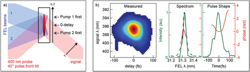
Although the mini-TIMER setup works at small values of $2\theta$, the smearing of the arrival time at the sample surface can be used to implement single-shot cross correlation measurements of the FEL pulse in a frequency resolved optical gating (FROG) configuration, as depicted in Figure 30 a) [273]. On one side of the interaction region the probe sees pump 1 first and pump 2 after, on the other side it is the other way around and only the centre corresponds to time zero. If the wave front of the probe is previously tilted to be parallel to the sample surface, it becomes possible to map the time delay as a function of the position along the detector where the interaction region is imaged. Moreover, dispersing the signal along the opposite direction with a grating allows to simultaneously map the frequency and extract single shot FROG images of the FEL pulses, as the one shown on the left of Figure 30 b). A successive reconstruction allows the extraction of shot by shot spectral and temporal shape of the pulses, as depicted on the right, where the intensities are plotted in green and their corresponding phases in red.

5.3 The TIMER system: exciting and probing EUV TG in the sub-100 nm scale

The TIMER instrument was designed to perform full EUV TG experiments, overcoming the limitation in the achievable $L_{TG}$ intrinsic of TG experiments involving optical pulses. The setup is depicted in Figure 31a, and is based on a fully reflective scheme to split and recombine the beams over a broad wavelength range. A plane mirror (PM1) is inserted vertically to reflect the probe beam half. The transmitted half constitutes the pump branches after being split, this time horizontally, by a second planar mirror (PM2).

Figure 31. a) Schematic drawing of the beamline. SM: switching mirror from the FERMI transport. PM1: plane mirror beam splitter dividing vertically the probe beam from the excitation beams. PM3,4: plane steering mirrors for the probe beam. PM2: plane mirror beam splitter separating horizontally the two excitation beams. 1A to 4A: focusing toroidal mirrors for the pump A. 1B to 4B: focusing toroidal mirrors for the pump B. 1P to 4P: focusing toroidal mirrors for the probe. $2\theta$: excitation crossing angle. ${\theta }_{\text{B}}$: probe incidence angle. Δt_A,B: indicates the relative delay between the two excitation beams. Δt: indicates the relative delay between excitation and probe. b) values of ${\text{L}}_{\text{TG}}$ as a function of ${\lambda }_{\text{pump}}$ for the case of FEL2. The different colours correspond to the four possible probe wavelengths (6.7- red, 8.34 - green, 13.3 - blue and 16.7 nm - black). The shapes indicate the four crossing angles: 18.4° - square, 27.6° - triangle, 79° - inverted triangle and 105° - circle. c) Values of ${\text{L}}_{\text{TG}}$ as a function of ${\lambda }_{\text{pump}}$ for the case of FEL1. The different colours correspond to the two available probe wavelengths (17.8 - blue and 20.6 nm - red). The shapes indicate the four crossing angles: 18.4° - square, 27.6° - triangle, 79° - inverted triangle and 105° - circle.

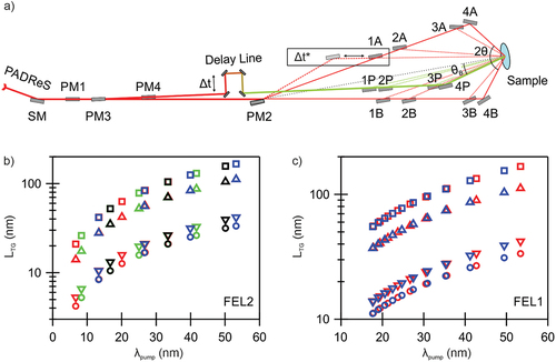
Then, the two pump beams (A and B, respectively reflected and transmitted) are recombined at the sample by sets of focusing toroidal mirrors (TM; 1–4 A and B in Figure 32 a), each hosted in a separate vacuum chamber and selected by vertical translation. The design allows for four possible pump crossing angles $2\theta =$ 18.4°, 27.6°, 79° and 105.4°. The temporal overlap is controlled by a translation of the TM of the branch A along the propagation direction, to conserve the incidence angle, and a corresponding pitch of PM2 and the TM itself, as schematized in Figure 31 a). In this way, the relative delay between the two pump pulses can be varied between −3 and + 7 ps with 1 fs precision but unfortunately with low mechanical reproducibility. The arrival time of the two pulses with respect to a reference optical laser pulse can be determined with ≈ 10 fs precision by EUV-optical pump-probe measurements, using the low-jitter optical laser system available at all beamlines of the FERMI FEL [274,275].

Figure 32. a) Transmission of the filters available along the pump beams transport. b) Transmission of the filters available in front of the detector. The arrows in both panel a) and b) indicate that, for an exemplary choice of λ_pump = 26.6 nm and λ_probe = 13.3 nm, a proper choice of filters allows for an almost full extinction of the probe along the excitation transport and of the pump scattered light at the detector. c) Transmission of the pump branch-line a (straight lines) and B (dashed lines) for the four crossing angles. 18.4° - red, 27.6° - blue, 79° - green and 105°- black. The two pump branch-line differ by the reflectivity of the splitting mirror PM2. d) Transmission of the probe beam for the four crossing angles (same colours as in panel c) without the delay line inserted.

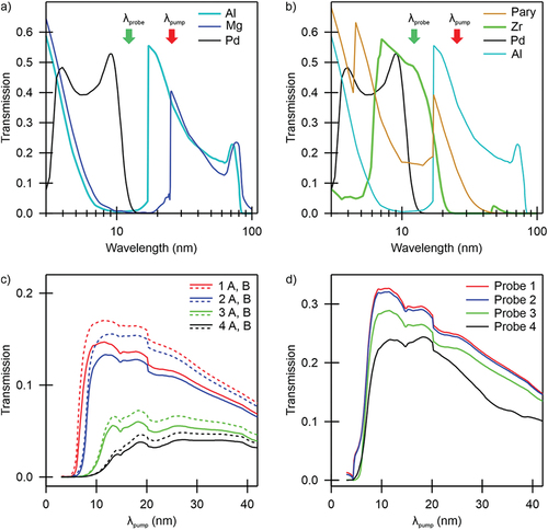
The vertically-split probe is steered back to be coplanar with the pump beams by two plane mirrors (PM3 and PM4) before reaching the delay line, used to precisely set its arrival time with respect to the pump. In order to investigate dynamics that last from a few femtoseconds to nanoseconds, the TIMER delay line is designed with four multilayer mirrors at 45° angle of incidence. This choice is made at the expenses of a broad tunability in ${\lambda }_{probe}$, which is limited to the design wavelength of the mirrors. The delay line is equipped with four sets of mirrors, currently at 8.34, 13.3, 16.7 and 20.6 nm. 6.7, 17.8 nm or other user-provided mirrors can be mounted upon request. Table 1 summarizes the main parameters for each set of mirrors.

Table 1. Parameters of the ML mirrors available for the TIMER delay line, summarising central wavelength ${\lambda }_{\text{probe}}$ , bandwidth $\mathrm{\Delta }{\lambda }_{\text{probe}}/{\lambda }_{\text{probe}}$ and transmission of the delay line after a full set of 4 mirrors. In bold the sets currently in use.

${\mathit{\lambda }}_{\mathit{p}\mathit{r}\mathit{o}\mathit{b}\mathit{e}}$	$\mathbf{\Delta }{\mathit{\lambda }}_{\mathit{p}\mathit{r}\mathit{o}\mathit{b}\mathit{e}}/{\mathit{\lambda }}_{\mathit{p}\mathit{r}\mathit{o}\mathit{b}\mathit{e}}$	Transmission
20.6	0.068	0.08
17.8	0.09	0.09
16.7	0.083	0.15
13.3	0.041	0.2
8.34	0.011	0.014
6.7	0.008	0.08

The condition on ${\lambda }_{probe}$ dictates the whole geometry of the beamline, designed to achieve Bragg conditions for ${\lambda }_{pump}=3{\lambda }_{probe}$. This also determines the incidence angle of the probe: ${\theta }_{probe}=$ 3.05°, 4.56°, 12.24° and 15.38°. Similarly to the pump branch lines, the probe beam is focused at the sample at the desired angle by using 1 of the 4 selectable TMs (1–4 P). It is worth mentioning that the combinations ($2\theta ,{\theta }_{probe})=\left({18.6}^{\circ },{4.6}^{\circ }\right)$ and $\left({27.6}^{\circ },{12.2}^{\circ }\right)$are not possible because of mechanical conflicts. We recall that the Bragg condition permits to maximise the signal intensity and, as shown in Equation 7(7) $\begin{array}{ll}F\left({\lambda }_i,{\theta }_i,L_i,d\right)=& \frac{cos{\theta }_{sig}}{cos{\theta }_{probe}}{\left[\pi n\left({\lambda }_{probe}\right)d/{\lambda }_{probe}cos\left({\theta }_{probe}\right)\right]}^2\\ & \times \frac{e^{-\left(d/2L^{\ast }\right)}-2cos\left(\mathrm{\Delta }{K}_{z}d\right)e^{-\left(d/2L^{\ast }\right)}+1}{{\left(d/2L^{\ast }\right)}^2+{\left(\mathrm{\Delta }{K}_{z}d\right)}^2}{e}^{-d/L_{abs,probe}cos{\theta }_{sig}},\end{array}$(7) , might be indispensable in low absorbing samples at short $L_{TG}$. Figure 31 b) plots the achievable values of $L_{TG}$ considering the FERMI FEL2 source with ${\lambda }_{pump}=N{\lambda }_{probe}$, where N is an integer number. Figure 31 c) shows the same plot when ${\lambda }_{probe}$ is in the FERMI FEL1 range, and${\lambda }_{pump}=\left(N_1/N_2\right){\lambda }_{probe}$, where N₁ and N₂ are integer numbers. In Figure 31 b) and c) we do not report ($2\theta ,{\lambda }_{pump},{\lambda }_{probe}$)-combinations that do not fulfil Equation 2(2) $L_{TG}={\lambda }_{pump}/\left[2sin\left(\theta \right)\right].$(2) and Equation 4(4) $L_{TG}\left[sin\left({\theta }_{sig}\right)+sin\left({\theta }_{probe}\right)\right]={\lambda }_{probe},$(4) for any of the available values of ${\theta }_{probe}$. Moreover, about 70% of these points do not fulfil Bragg conditions, here EUV TG experiments are still viable in many practical cases.

The experience gained so far indicates that the use of the two stages of FEL2 is preferable, since a more stable FEL operation can be achieved and it is easier to independently regulate the intensities of the pump and probe beams. In addition, to vary $L_{TG}$ it is generally preferred to work at a fixed value of $2\theta$ and exploit the capability of FERMI to flexibly change FEL wavelengths, in order to minimise the dead times. Normally, the pump is set at the longer wavelength (and the instrumental geometry is designed accordingly) because the $L_{abs}$ increases on decreasing $\lambda$, favouring the probe’s transmission through the sample, if no absorption edges are present between ${\lambda }_{pump}$ and ${\lambda }_{probe}$. However, for a subset of ($2\theta ,{\theta }_{probe}$) combinations, it is possible to work in the condition ${\lambda }_{pump}<{\lambda }_{probe}$. The use of different wavelengths for exciting and probing the EUV TG allows employing filters for increasing the S/N. In fact, although in principle TG spectroscopy is background free since the signal is scattered at large angles with respect to the transmitted pump and probe beams, the EUV TG signal can be on the same intensity level as the straylight coming from the beamline or spurious scattering from surface roughness. Moreover, the signal decay often contains important dynamical information, e.g. on the phonon decay (see sections 4.2.1 and 4.3), therefore the S/N plays a critical role to determine the EUV TG waveform at long $\mathrm{\Delta }t$, when the signal is much weaker. Figure 32 a) and b), display the transmission of the (solid-state) filters that can be inserted, respectively, in front of the detector and along the pump branch-lines; other kinds of filters can be installed if needed. For example, when ${\lambda }_{pump}$ and ${\lambda }_{probe}$ are respectively set to 26.6 and 13.3 nm (red and green arrows in Figure 32 a), and Figure 32 b), the spurious radiation at ${\lambda }_{probe}$ that propagates along the pump branch-lines can be removed by the Al filter and the radiation at ${\lambda }_{pump}$ scattered by the sample roughness is strongly attenuated by the Zr filter at the detector. The only remaining source of spurious background is due to diffuse scattering of the probe beam.

Figure 32 c) and d) display the transmission of the pump and probe branch-lines, respectively. The transmission decreases at short wavelengths, stronger when larger angles are involved ($2\theta$: 79° and 105.4°). This makes reaching the shorter values of $L_{TG}$ shown in figure 31 b) very difficult. Special multilayer coatings can be realised on the TMs to mitigate this issue in a specific wavelength range, at the price of reducing the transmission outside this range. We mention that for each TM holder there is the possibility to swap between two mirrors, one with the conventional coating (resulting in the transmissions displayed in figure 32 c) and d) and another one, that is presently is a blank substrate but could host the required special multilayer coating.

5.3.1 Sample environment and EUV signal detection

The samples are hosted in the main experimental chamber on a 6-axis manipulator with three translational degrees of freedom (x, y, z, as defined in Figure 28d) and 3 rotations: $\theta$ around the y axis, $\phi$ around the x axis and ${\theta }^{\prime }$ around an axis lying in the yz plane and decoupled from the other rotations. Around the sample there are about 20 cm to host different sample environments. For example, it is possible to mount a cryostat coupled to the sample holder through a copper braid to cool the sample down to 40 K. Also, the sample can be kept in a magnetic field with the help of permanent magnets mounted either to special manipulator plates (with fields both perpendicular and parallel to the sample surface) or onto translational stages for variable fields perpendicular to the sample surface. Additionally, a cylindrical electromagnet with an on-axis field of ±80 mT was designed ad-hoc for the TIMER experiment (see Figure 33 b). It features a clear aperture of 120° to accommodate the largest pump crossing angle and most of the signal scattering angles, a 10 mm gap between coils to host the sample holder and a central hole aperture of 20 mm.

Figure 33. a) Sketch of the standard setup in the experimental chamber, when two CCD detectors are used to collect forward and backward diffracted signal. It is possible to use a single detector by installing it on a mechanical stage with sufficient stroke, but in this case the two signals cannot be acquired simultaneously. The optical laser beam and the detector normally used for timing the FEL pulses via EUV-optical pump-probe measurements are also sketched; detection in reflection geometry and signal polarization analysis (not shown) are also available. b) Picture of the electromagnet installed in the sample area. c) Picture of the standard setup for the detection of the backward diffracted EUV TG signal.

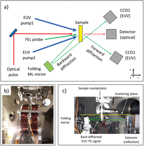
As sketched in Figure 33 a), TIMER is equipped for TG signal detection both in forward (Detector1) and in backward diffraction (Detector2) using two identical CCDs. Both detectors are hosted on translational stages to centre them at the signal position. The backwards scattering detection setup is depicted in Figure 33 a) and c), respectively from the top and from the side. To work in backscattering geometry the sample is tilted around the x axis by 10°, such that the signal can be picked by a multilayer mirror (ML) located below the scattering plane. This folding mirror reflects at almost normal incidence onto the detector placed behind the sample. This choice minimises both the lateral dimensions of the setup and the footprint of the signal on the detector. MLs are available for all probe wavelengths indicated in Table 1 and can be mounted in pairs inside the vacuum chamber to reduce downtime in case of wavelength changes. The drawback of normal-incidence schemes is that the reflectivity of both sample and ML mirror decreases drastically with decreasing wavelength. Schemes at grazing incidence can be employed in this case and are described elsewhere [197].

5.3.2 Polarization analysis of EUV TG signals

As discussed in section 3.4.4 for the case of magnetic samples and later on for other applications such as chiral molecules, sometimes it can be useful to selectively choose the signal polarisation to be detected. In the EUV regime, due to the lack of transmission optics, this is not a trivial task and is usually solved by exploiting the radically different reflectivity for s and p polarisation (see Figure 34 a) close to the Brewster angle, which in the EUV and X-ray range is close to 45°. Since the TIMER delay line transmits only vertical polarisation, i.e. on the xy plane, a mirror reflecting vertically at 90° will almost only reflect the rotated component, i.e. on the scattering plane as depicted in panel b) of Figure 34, and suppress the light with the original polarisation direction. The setup for polarisation analysis is depicted in Figure 34 c). It consists of one ML mirror at 45° that reflects the rotated signal onto a CCD detector (labelled as CCD A in the figure), while the total signal consisting of both the rotated and unrotated polarization components can be measured by another CCD (labelled as CCD B in Figure 34). Note that this setup does not allow to simultaneously measure both components but requires two subsequent measurements. Schemes for the simultaneous detection of s and p polarizations are currently being developed at other FERMI endstations [276,277].

Figure 34. a) Representative reflectivity of a ML mirror at 45° angle incidence as a function of $\mathit{\lambda }$ for S-polarized (black curve) and P-polarized (red curve) radiation; a moderate extinction ratio of about 20 is achieved. This specific mirror is used in combination with the ML set at 20.6 nm in the EUV delay line (see Table I). b) Sketch of the polarization analysis scheme. c) Picture of the standard setup for polarization analysis of the EUV TG signal. The two detectors are mounted on motorized stages and can be interchanged, in order to acquire (not simultaneously) the polarized and unpolarized EUV TG signals.

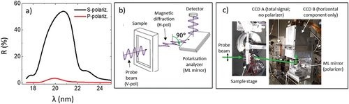
6 Perspectives

The first observation of EUV TG response has been possible thanks to the intense pulses produced by FERMI and, for this reason, is a relatively recent achievement [269]. Nonetheless, as reported in the previous sections, a consistent number of experiments carried out in various research fields demonstrates the great potential of this methodology, in particular to the broad research fields of nanoscale transport phenomena, ultrafast magnetism and elasticity. There are several future developments that will further extend the range of possible applications of transient grating at sub-optical wavelengths both from the point of view of investigated materials and of accessing to experimental conditions not yet fully exploited, which may enable to realize experiments based on the unique capability to control the interference of ultrafast EUV pulses.

6.1 Beyond “conventional” EUV TG

This is for example the case of crossing orthogonally polarised beams that produce, instead of the typical periodic intensity pattern (see Figure 35a), a periodic pattern of circular left, linear and circular right polarisation on top of a constant intensity profile, as shown in Figure 35b. This pattern could be beneficial to detect weak chiral centres by combining the difference in the absorption of dichroic molecules with the background-free detection capabilities peculiar to the transient grating technique [278]. The constant intensity profile will give rise to a non-modulated background which thus will not contribute to the signal. Moreover, exploiting core hole excitations, transient polarization gratings would permit carrying out resonant natural dichroism measurements that are particularly suited to monitor the local molecular chirality [279]. Magnetism as well could take advantage of the polarisation TG where spin waves are directly excited [280] without being coupled to thermal or magnetoelastic phenomena.

Figure 35. Spatial patterns of light intensity (red line) and polarization (thin black arrows) generated by two crossed beams (thick red arrows) with parallel (Panel a) and orthogonal polarization (Panel b). In the first case the light polarization is constant and parallel to the one of the excitation beams, in the second case the light intensity is constant while the polarization changes from linear, to right circular, linear rotated by 90 degree, left circular and so on.

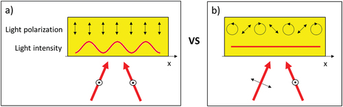
One more high-potential application of EUV TG is provided by the possibility of measuring the self-diffracted intensity of the pump beams, i.e. the scattering of the pump pulses by the grating that they generate, as shown in Figure 36. Not requiring the probe pulse and resulting in a wavelength independent emission angle, self-diffraction greatly simplifies the experimental design, enabling to easily vary the wavelength and exploit the background free power of TG, with the potential to identify structures normally hidden by the S/N in standard X-ray absorption spectroscopy (XAS) experiments or to access states normally forbidden by selection rules for single photon interactions. Moreover, as detailed above, TG accesses the squared modulus of the complex refractive index variation, while XAS is only sensitive to its imaginary part. Measuring simultaneously the XAS and the self-diffracted signal may lead to a new way of determining the EUV/X-ray refractive index, e.g. without the need to solve the Kramers-Kroening relations.

Figure 36. a) Experimental scheme for self-diffraction. Here the FWM signal is given by the diffraction of the pump beams by the grating they generate. The figure shows the first positive and negative diffraction orders of the beam propagating along P₁. The order m = +1 co-propagates with the transmitted beam along P₂. Placing two detectors into these directions allows measuring the XAS from P2 beam and the self-diffraction of P1 beam. b) Exploiting the FEL polychromatic emission opens the way to more complex schemes where the frequency of the diffracted signal is given by a linear combination of the ones of the incoming beams, thus being separated from the transmitted intensity.

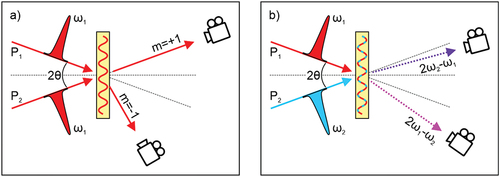
Furthermore, the scheme in Figure 36a, only requires a split and recombination system for the pump pulses, making it easier to extend other types of FWM techniques to the EUV/soft X-ray regime. In this context, an additional perspective is enabled by the capability of FELs to generate a two colours output (${\omega }_1$,${\omega }_2$), which can be splitted and recombined at the sample using the noncollinear setup adopted for EUV TG, as sketched in Figure 36b. This enables coherent anti-Stokes Raman scattering (CARS) [281,282], a powerful and fascinating technique where the time dependent ‘beatings’ at ${\omega }_1-{\omega }_2$ occuring during the pulsed illumination of the sample selectively drive sample excitations at a selected frequency ${\omega }_{exc}={\omega }_1-{\omega }_2$ and wavevector $\mathrm{\Delta }{k}_{exc}=|k_1-k_2|$. A third pulse of frequency ${\omega }_3$ (typically with ${\omega }_3={\omega }_1$), interrogates the system and generates a signal of frequency ${\omega }_1-{\omega }_2+{\omega }_3$. Such a Raman-shifted signal, emitted in the phase matched direction, encodes information on the generated excitations that, in optical CARS, are typically limited to vibrational modes. The use of EUV/soft X-ray photons can enlarge the exploitable range to valence-band electronic excitations, in addition, the use of core resonances allows to add chemical selectivity. The extension of CARS-like approaches to the soft X-ray was actually theoretically envisioned and its great potential still represents one of the stronger general motivations for X-ray FWM [231]. In a simple scheme like the one shown in Figure 36b, one may actually detect FWM signals at $2{\omega }_1-{\omega }_2$ or $2{\omega }_2-{\omega }_1$; indeed multicolor wave mixing signals have recently been observed [283,284]. Furthermore, the additional ability of FERMI to control the relative phase of multi-colour FEL pulses [211–213] may open the way of studying sub-fs phenomena in materials, such as electrons and/or energy transfer between different atomic species.

The non-collinear scheme provided by the EUV TG setups can also be exploited for imaging. For instance, when the two crossed beams are brought into interaction with an object they generate two diffraction patterns corresponding to two distinct illumination angles. Collecting simultaneously these two patterns the 3D structure of the object can be reconstructed, providing the basis for ultrafast 3D imaging with sub µm resolution [285]. The periodic illumination of the sample offers another potential breakthrough for imaging, that is to notably push forward the limit of structured illumination microscopy (SIM) [286]. This technique makes use of a sinusoidally shaped laser beam to image structures below the Abbe limit. The spatial wavevector ($k_b$) defined by the sinusoidal profile of the illuminating light interferes with the characteristic spatial wavevectors of the sample ($k_s$) and gives rise to Moiré fringes at ($k_b-k_s$), thus extending the maximum observable value of $k_s=k_{max}$ (that ultimately defines the spatial resolution) by an amount equal to $k_b$. This is sketched in Figure 37b), where the blue circle represents the range $k_s⩽k_{max}$ accessible by standard (Abbe limited) microscope, while the yellow circles are translated by $\left|k_b\right|$. The partial overlap between blue and yellow circles gives rise to the Moiré fringes that act as a reference to reconstruct the image, permitting access to a larger range in $k_s$. Optical TG excitation naturally provides sinusoidal illumination, though limited to values of $k_b\approx k_{max}$, which implies an increase in $k_s$ (and thus in the spatial resolution) of about a factor 2. This limitation can be removed using EUV TG, where in principle $k_b$ can be continuously varied from values $k_{max}$ up to the inverse nanometer range, in $k_b$-steps sufficiently small to preserve the overlap in $k_s$-space, as shown in Figure 37c). We recently used EUV TG to detect Moiré fringes obtained by illuminating a material grating of 260 nm period with a EUV TG of L_TG = 270 nm, in this case the Moiré pattern is a simple grating with 6.6 µm period that can be easily imaged by using a standard microscope objective.

Figure 37. Panel a) reports a sketch of standard SIM microscopy. Blue circle represents the spatial frequencies ${\text{k}}_{\text{s}}<{\text{k}}_{\text{max}}$ accessible by an optical microscope, while yellow circles are those accessible by using a sinusoidal structured illumination with characteristic wavevector ${\text{k}}_{\text{b}}$. The overlap areas give rise to the Moiré pattern. Using optical TGs the value of ${\text{k}}_{\text{b}}$ is on the same order as ${\text{k}}_{\text{max}}$. Panel b) illustrates the possibility to use EUV TG to progressively increase the accessible range in ${\text{k}}_{\text{s}}$ while maintaining the overlap in $\text{k}$-space.

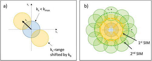
6.2 Beyond the EUV range

Though X-ray TG excitation has been recently demonstrated [227], the capability to both excite and probe the TG with short wavelength radiation is nowadays limited to the EUV range. This prevents reaching single-digit nm values for $L_{TG}$ and also limits spectroscopic applications to the few material edges lying in the EUV range. Single digit nm TGs can be extremely relevant for phenomena where the nuclear and electronic degrees of freedom are non-independent, like charge density waves. The current limit in $L_{TG}$ for the EUV TG instrument at FERMI is $\approx$ 13 nm, though the shortest value used so far is 16.7 nm; see Figure 18a). This limit is imposed by the insufficient reflectivity of the focusing toroidal mirrors (see Section 5.3) at large angles and short wavelengths. This problem can be mitigated by the constantly improving multilayer coating technology, which can be applied to toroidal mirrors to increase the reflectivity in a selected wavelength range. In the case of the TIMER instrument this would imply the possibility of reaching $L_{TG}\approx$ 6 nm, yet with the limitation of a small working range ${\lambda }_{pump}$ and, obviously, without solving the wavefront tilt issue (see Section 5.1). These limitations could be overcome by using X-ray diffractive optics (XDOs) to realize the X-ray analogue of the instrumental concept commonly used in optical TG [144]. The essence of this scheme is illustrated in Figure 38 b): a focusing zone plate (FZP) generates an X-ray spot on a phase mask (PhM), which is then imagined at the sample position by two off-axis zone plates (OAZP). Based on the current PM technology and possibly exploiting demagnification with properly designed OAZPs, sub-10 nm TG periodicities could be achieved, and the wavefront tilt issue is radically solved since the interfering pulses have parallel wavefonts at the sample. Remarkably, the use of these XDOs to manipulate the beam becomes more effective in the X-ray region, where the absorption of materials is lower and precise structures can be manufactured, thus potentially enabling the combination of nanoscale TGs with X-ray spectroscopy. A first step in this direction was made by using the X-ray Talbot effect, where a diamond PM was used to create a µm scale X-ray TG excitation, still without the possibility of X-ray probing [227]. In Figure 38b), we assume that the probe beam is another X-ray pulse (focused at the sample with the desired angle by OAZP_pr) parallel but not collinear with the pump beam impinging on FZP and PhM, which is possible to obtain with X-ray split-delay units. These devices can actually generate parallel X-ray beams with a variable delay, though with a little lateral separation; in principle this can be enlarged by a slightly different mechanical design.

Figure 38. Comparison between the all-reflective split-recombination principle presently used presently system used at the EUV TG instruments of FERMI (Panel a); same as Figure 28b) versus the one based on XDOs: FZP, PhM and OAZP. FZP generates an X-ray spot at PhM, which is imaged at the sample position by OAZP1 and OAZP2. This scheme will provide both equal intensity interfering pulses and parallel wavefronts at the sample position. A third OAZP (OAZP_pr in the sketch) can be used to focus the EUV/X-ray probe beam at the sample.

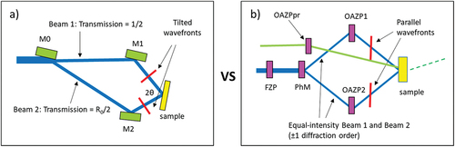
An interesting possibility offered by setups based on DOEs is to use purposely designed elements to generate more complex spatial excitation patterns, such as 2D gratings. Generation of ultrafast and nanoscale 2D patterns of light intensity would permit, e.g. to drive the nucleation of skyrmions in magnetic materials, whose dynamics would be probed by transient diffraction of the X-ray probe pulse.

6.3 Beyond solid state samples

Another natural step would be to extend the TG/FWM approach to gas phase samples. This would be of fundamental importance to investigate the basics of EUV/X-ray nonlinear optics and compare them with existing literature. As a matter of fact, the majority of theoretical works on EUV/X-ray nonlinear optics consider isolated and non-interacting molecules [229–231], i.e. gas phase samples. These samples are actually at the reach of present capabilities. Indeed, an order of magnitude estimate of the expected signal from gas phase samples can be made in comparison to what observed from solid state ones. The main differences are the sample density and thickness. To simply illustrate the effects of these two parameters, one can consider that in standard conditions helium has a density of about 1.7 × 10⁻⁴ g/cm³ , which is about 3 × 10³ times lower than lithium, the closest solid-state element in the periodic table. According to Equation 14(14) $\frac{\partial n\left(\lambda \right)}{\partial \rho }\mathrm{\Delta }\rho =\mathrm{\Delta }{n}_{\rho }\left(\lambda \right)=\left(\frac{r_e{\lambda }^2}{2\pi }f{}^{\prime }\left(\omega \right)+\frac{i{r}_e{\lambda }^2}{2\pi }f{}^{\prime \prime }\left(\omega \right)\right)\mathrm{\Delta }\rho =\left(\delta +i\beta \right)\frac{\mathrm{\Delta }\rho }{\rho }$(14) , this leads to a lower EUV TG signal by about 7 orders of magnitude. However, given the lower sample density, the sample thickness can be increased. For instance, for ${\lambda }_{pump}=$ 40 nm $L_{abs,pump}=$ 8 µm in helium and 0.8 µm in lithium. Assuming a spot size of 100 µm and beam crossing angle of about 10 deg, the spatial overlap of the interfering pulses is maintained along a sample thickness exceeding 8 µm and the quadratic dependence of the EUV TG signal from the sample thickness, might thus lead to 2 orders of magnitude more signal from the gaseous sample. In addition, gas phase samples do not suffer from sample damage and pump pulse energies exceeding 100 µJ can be envisioned, while in solid state samples pulse energies of about 1 µJ on 100 µm spot sizes typically already result in sample damage. The quadratic dependence of the EUV TG signal on the excitation fluence will thus lead to another 4 orders of magnitude in favour of the gas sample, overall balancing the 7 orders of magnitude lost because of the lower density. A more quantitative estimate can be done by considering the electronic signal observed from cobalt and shown in Figure 18b). Here ${\lambda }_{pump}=$ 20.8 nm, $L_{abs,pump}=$ 11 nm and the density was 8.9 g/cm³, scaling these numbers on the aforementioned helium density (and considering the different values of Z) one can expect a EUV TG signal decrease by a factor about 4 × 10³ for the same excitation fluence, on using helium instead of cobalt; a factor 100 increase in the excitation fluence could thus lead to an even larger EUV TG signal from the gaseous sample. However, this order of magnitude estimate does not consider high-field effects, which may alter significantly the molecules under investigation. On the other hand, the possibility to study such effects in FWM processes represents per se an interesting scientific opportunity.

Before moving to the conclusions, we mention possible industrial applications of the TG: the development of XDO-based TG, combined with bright HHG sources and possibly with µm-focusing capabilities, can lead to significantly more compact setups deployable by industry (other than being usable in academic and research laboratories, beyond the context of large scale research infrastructures where the method was pioneered). As shown in this review, TG can access a variety of nanoscale phenomena ranging from magnetism to heat diffusion and elasticity, which can be of great help in characterising and developing new materials or architectures for efficient computing and data storage. Moreover, similarly to what has been successfully implemented with other experimental techniques, such as Raman, Brillouin and optical TG, compact sub-100 nm TG setups based on HHG and driven by ‘turnkey’ lasers can be developed to become a diagnostic tool to map, point wise, material properties.

7 Conclusions

The advent of Free Electron Lasers provided the scientific community with short-wavelength, intense, coherent, ultrashort and tunable pulses. These features enabled nonlinear optical and spectroscopic methods in the short wavelength range, analogous to what occurred with terahertz to ultraviolet nonlinear optics over the past sixty years. The wavelength range of core-transitions provides element-specificity, orbital-selectivity, structural resolution down to the sub-nanometer scale and high momentum transfers. In addition, polarisation control and high temporal (attosecond to femtosecond) resolution open up new horizons in nonlinear optics and spectroscopy. This review is meant to describe the progress of this nascent field over the past ten years focussing on the results obtained extending the transient grating method, a third order nonlinear optical process, to the short-wavelength range accessible by the FERMI free electron laser.

Transient grating spectroscopy is an elegant method that uses two pulses to excite the medium producing a standing wave. Instead of the uniform excitation of the surface produced by a single pulse, the excitations are thus organised into parallel stripes. A third pulse is used to monitor the evolution in time of the modulation created by the pump pulses. The advantage to have scattered intensity only at the Bragg angle makes this technique extremely sensitive. The temporal evolution of the excited grating depends on many factors such as the sample material and the wavelength, intensity and polarisation of the pump pulses. We demonstrated how the use of short wavelength pulses provided by free electron lasers has brought the transient grating approach to the next level, allowing us to investigate nanoscale dynamics in a variety of systems of paramount importance for the condensed matter scientific community. The high sensitivity of the technique allows working with fluences which do not cause significant changes in the sample. One of the major limitations of the use of FELs in the study of materials of interest for condensed matter science is in fact often linked to the need to irradiate the sample with high-intensity pulses in order to obtain a good signal-to-noise ratio.

Understanding the dynamics at the nanoscale is at the basis of the advance towards new functional materials such as miniaturised thermal devices, superconductors, ultrafast magnetic switches, photocatalysts and ultrafast data storage elements. For instance, the study of thermal transport at the nanoscale is extremely important and is mostly motivated by current needs as, for example, the thermal management of micro/nano-electronic devices. Chip-level hotspots are troubling microelectronic designers who encounter severe thermal management problems at nanometer-length scales within individual transistors. When the mean free path of heat carrying phonons becomes larger than the hot spot regions the conventional heat diffusion theory does not apply and the so-called ballistic regime is reached. The general consensus is to shift towards novel, confined device geometries (ultrathin body, nanowires) and lower thermal conductivity materials (e.g. germanium). This will add complexity and motivate new methodologies to device design focused on nanoscale conduction physics coupled to electron and phonon transport modelling. In this scenario transient grating experiments are able to characterise thermal diffusion at the nanoscale as we demonstrated in [6]. Femtosecond All-Optical Switching (AOS) represents another hot area of research due to the interesting and potential application in the next generation of information technology. In the last years the understanding of the temporal control of AOS has progressed rapidly but it needs to be expanded into the nanometer range, where ultrafast lateral transport processes are expected to ultimately compete with AOS. Recently the transient grating approach has been employed to demonstrate the emergence of AOS on the nanometer length scale in a GdFe sample by looking at the nonlinear demagnetization response as a function of excitation fluence, a fingerprint of AOS, via the ratio between the second and first order diffraction intensities [215]. We mentioned these two examples of successful studies that manifest the enormous potential of the transient grating technique in material science.

Future investigations may span from multiferroic materials, to the study of chiral molecules. Multiferroics compounds exhibit order both in their magnetic and electronic systems. The existence of these multiple simultaneous interacting forms of order suggests that their dynamics might be related, and that an optical stimulus can provide the means to control both forms of order. Controlling the magnetic order in multiferroic materials is of particular interest due to potential applications in devices employing the dynamics of magnetism at the nanometer scale, termed spintronics. The frontier of spintronics involves developing the means to control magnetic order by electric fields at very short timescales. However, the underlying physics and ultimate speed of magnetoelectric coupling needed for this control remains largely unexplored. Concerning chiral molecules, transient polarisation grating may be employed to measure the X-ray natural circular dichroism and, exploiting the highly localised nature of core excitations, makes it an ideal probe of local chirality within molecules, providing a new method for chemical and biochemical analysis. Due to the low signal that can be obtained using linear spectroscopies such as absorption at synchrotrons, to date no X-ray natural circular dichroism studies have been performed on solutions, even though liquids are the natural medium of (bio)chemistry. Furthermore, for the latter, the detection of light elements (C, N, O,…) and of transition metals and their evolution in the course of a reaction are of central importance. Transient grating is one of four wave mixing nonlinear effects arising from a third-order optical nonlinearity. The results and perspectives discussed in this review allow us to imagine what repercussions may have the extension of all methods based on nonlinear optics at the short wavelength region accessible now by free electron lasers.

Disclosure statement

No potential conflict of interest was reported by the authors.

Appendix A

List of acronyms

Table

AOS	All-optical switching
BLS	Brillouin light scattering
CARS	Coherent anti-Stokes Raman scattering
CCD	Charge coupled detector
CL	Circular left
CR	Circular right
DECP	Displacive excitation of coherent phonons
EUV	Extreme ultraviolet
FEL	Free electron laser
FWHM	Full width at half maximum
FM	Folding mirror
FROG	Frequency resolved optical gating
FZP	Focusing zone plate
FWM	Four wave mixing
HHG	High harmonic generation
INS	Inelastic neutron scattering
IXS	Inelastic x-ray scattering
LA	Longitudinal acoustic
LINAC	Linear accelerator
ML	Multi-layer
OAZP	Off-axis zone plate
PM	Plane mirror
PhM	Phase mask
RLS	Raman light scattering
S/N	Signal to noise ratio
SASE	Self-amplified spontaneous emission
SAW	Surface acoustic wave
SIM	Structured illumination microscopy
SSLW	Surface skimming longitudinal wave
TA	Transverse acoustic
TG	Transient grating
XAS	X-ray absorption spectroscopy

References

- Kittel C. Introduction to solid state physics. Global edition, [9th ed. Hoboken, NJ: Wiley; 2018.
- Grüneisen E. Specific heat. Zusammenhang Zwischen Kompressibilität Thermischer Ausdehnung Atomvolumen Atomwärme Met. Ann. d. Phys. 1908;331:393.
- Leibfried G, Ludwig W. Theory of anharmonic effects in crystals. Solid State Phys. 1961;12:275–444.
- Casimir HBG. NoTe on the conduction of heat in crystals. Physica. 1938;5:495.
- Johnson JA, Maznev AA, Cuffe J, et al. Direct measurement of room-temperature nondiffusive thermal transport over micron distances in a silicon membrane. Phys Rev Lett. 2013;110:025901.
- Bencivenga F, Mincigrucci R, Capotondi F, et al. NanoScale transient gratings excited and probed by extreme ultraviolet femtosecond pulses. Sci Adv. 2019;5:eaaw5805.
- Kittel C. Interpretation of the thermal conductivity of glasses. Phys Rev. 1949;75:972.
- Schirmacher W. TheRmal conductivity of glassy materials and the “boson Peak”. Europhys Lett EPL. 2006;73:892.
- Martin JD, Goettler SJ, Fossé N, et al. Designing intermediate-range order in amorphous materials. Nature. 2002;419:381.
- Gibson JM, Treacy MMJ. DiminIshed medium-range order observed in annealed amorphous germanium. Phys Rev Lett. 1997;78:1074.
- De Gennes PG. Liquid dynamics and inelastic scattering of neutrons. Physica. 1959;25:825.
- Wu B, Iwashita T, Egami T. AtoMic dynamics in simple liquid: de Gennes narrowing revisited. Phys Rev Lett. 2018;120:135502.
- He Y, Donadio D, Galli G. Heat transport in amorphous silicon: interplay between morphology and disorder. Appl Phys Lett. 2011;98:144101.
- Zhou W, Cheng Y, Chen K, et al. TherMal conductivity of amorphous materials. Adv Funct Mater. 2020;30:1903829.
- Goodson KE. Ordering up the minimum thermal conductivity of solids. Science. 2007;315:342.
- Simoncelli M, Marzari N, Mauri F. UnifIed theory of thermal transport in crystals and glasses. Nat Phys. 2019;15:809.
- Fabian J, Allen PB. Anharmonic decay of vibrational states in amorphous silicon. Phys Rev Lett. 1996;77:3839.
- Braun JL, Baker CH, Giri A, et al. SIze effects on the thermal conductivity of amorphous silicon thin films. Phys Rev B. 2016;93:140201.
- Allen PB, Feldman JL. thermal conductivity of glasses: theory and application to amorphous Si. Phys Rev Lett. 1989;62:645.
- Mizuno H, Mossa S, Barrat J-L. BeatiNg the amorphous limit in thermal conductivity by superlattices design. Sci Rep. 2015;5:14116.
- Xie G, Ding D, Zhang G. Phonon coherence and its effect on thermal conductivity of nanostructures. Adv Phys X. 2018;3:1480417.
- Hoogeboom-Pot KM, Turgut E, Hernandez-Charpak JN, et al. NondEstructive measurement of the evolution of layer-specific mechanical properties in sub-10 Nm Bilayer films. Nano Lett. 2016;16:4773.
- Frazer TD, Knobloch JL, Hernández-Charpak JN, et al. Full characterization of ultrathin 5-Nm low- k dielectric bilayers: influence of dopants and surfaces on the mechanical properties. Phys Rev Mater. 2020;4:073603.
- Hernandez-Charpak JN, Hoogeboom-Pot KM, Li Q, et al. Full characterization of the mechanical properties of 11–50 Nm ultrathin films: influence of network connectivity on the poisson’s ratio. Nano Lett. 2017;17:2178.
- Beaurepaire E, Merle J-C, Daunois A, et al. UltRafast spin dynamics in ferromagnetic nickel. Phys Rev Lett. 1996;76:4250.
- Tauchert SR, Volkov M, Ehberger D, et al. Polarized phonons carry angular momentum in ultrafast demagnetization. Nature. 2022;602:73–77. DOI:10.1038/s41586-021-04306-4
- Dornes C, Acremann Y, Savoini M, et al. THe ultrafast einstein–de haas effect. Nature. 2019;565:209.
- Chen Z, Wang L-W. Role of initial magnetic disorder: a time-dependent ab initio study of ultrafast demagnetization mechanisms. Sci Adv. 2019;5:eaau8000.
- Ostler TA, Barker J, Evans RFL, et al. UltraFast heating as a sufficient stimulus for magnetization reversal in a ferrimagnet. Nat Commun. 2012;3:666.
- Battiato M, Carva K, Oppeneer PM. Superdiffusive spin transport as a mechanism of ultrafast demagnetization. Phys Rev Lett. 2010;105:027203.
- Reid AH, Shen X, Maldonado P, et al. BeYond a phenomenological description of magnetostriction. Nat Commun. 2018;9:388.
- Yazawa K, Leon Gil JA, Maze K, et al., Optical pump-probe thermoreflectance imaging for anisotropic heat diffusion, in 2018 17th IEEE Intersociety Conference on Thermal and Thermomechanical Phenomena in Electronic Systems (ITherm) (IEEE, San Diego, CA, 2018), pp. 59–66.
- Stanciu CD, Hansteen F, Kimel AV, et al. ALl-optical magnetic recording with circularly polarized light. Phys Rev Lett. 2007;99:047601.
- Mendil J, Nieves P, Chubykalo-Fesenko O, et al. Resolving the role of femtosecond heated electrons in ultrafast spin dynamics. Sci Rep. 2014;4:3980.
- Rudolf D, La-O-Vorakiat C, Battiato M, et al. UltraFast magnetization enhancement in metallic multilayers driven by superdiffusive spin current. Nat Commun. 2012;3:1037.
- Hofherr M, Häuser S, Dewhurst JK, et al. Ultrafast optically induced spin transfer in ferromagnetic alloys. Sci Adv. 2020;6:eaay8717.
- Willems F, von Korff Schmising C, Strüber C, et al. OPtical inter-site spin transfer probed by energy and spin-resolved transient absorption spectroscopy. Nat Commun. 2020;11:871.
- Göbel B, Mertig I, Tretiakov OA. Beyond skyrmions: review and perspectives of alternative magnetic quasiparticles. Phys Rep. 2021;895:1–28.
- Büttner F, Pfau B, Böttcher M, et al. ObservaTion of fluctuation-mediated picosecond nucleation of a topological phase. Nat Mater. 2021;20:30.
- Léveillé C, Burgos-Parra E, Sassi Y, et al. Ultrafast time-evolution of chiral néel magnetic domain walls probed by circular dichroism in x-ray resonant magnetic scattering. Nat Commun. 2022;13:1412.
- Kerber N, Ksenzov D, Freimuth F, et al. Faster chiral versus collinear magnetic order recovery after optical excitation revealed by femtosecond XUV scattering. Nat Commun. 2020;11:6304.
- Kirilyuk A, Kimel AV, Rasing T. Ultrafast optical manipulation of magnetic order. Rev Mod Phys. 2010;82:2731.
- Kirilyuk A, Kimel AV, Rasing T. Laser-induced magnetization dynamics and reversal in ferrimagnetic alloys. Rep Prog Phys. 2013;76:026501.
- CAN the U.S. COMPETE in basic energy sciences?, https://science.osti.gov/-/media/bes/pdf/reports/2021/International_Benchmarking-Report.pdf%20(2021).
- El Hadri MS, Pirro P, Lambert C-H, et al. Two types of all-optical magnetization switching mechanisms using femtosecond laser pulses. Phys Rev B. 2016;94:064412.
- Medapalli R, Afanasiev D, Kim DK, et al. Multiscale dynamics of helicity-dependent all-optical magnetization reversal in ferromagnetic Co/Pt multilayers. Phys Rev B. 2017;96:224421.
- Igarashi J, Remy Q, Iihama S, et al. EngineEring single-shot all-optical switching of ferromagnetic materials. Nano Lett. 2020;20:8654.
- Davies CS, Mentink JH, Kimel AV, et al. Helicity-independent all-optical switching of magnetization in ferrimagnetic alloys. J Magn Magn Mater. 2022;563:169851.
- Yamada KT, Kimel AV, Prabhakara KH, et al. EfficiEnt all-optical helicity dependent switching of spins in a Pt/Co/Pt film by a dual-pulse excitation. Front Nanotechnol. 2022;4:765848.
- Mukamel S. Principles of nonlinear optical spectroscopy. New York: Oxford University Press; 1995.
- Boyd RW. Nonlinear optics. 4th ed. San Diego: Academic Press is an imprint of Elsevier; 2019.
- Selenium and the Photophone. Nature. 1880;22:500. DOI:10.1038/022500a0
- Rolt KD. History of the flextensional electroacoustic transducer. J Acoust Soc Am. 1990;87:1340.
- Robbes D. Highly sensitive magnetometers—a review. Sens Actuators Phys. 2006;129:86–93.
- Eisenberg A, Eu BC. MecHanical spectroscopy: an introductory review. Annu Rev Mater Sci. 1976;6:335.
- Humphrey FB, Gyorgy EM. Flux reversal in soft ferromagnetics. J Appl Phys. 1959;30:935.
- Doyle WD, Flanderst PJ, He L, et al., MeasureMent of the switching speed limit in high coercivity magnetic media. In [1993] Digests of International Magnetics Conference (IEEE, Stockhom, Sweden, 1993), p. AB–AB.
- Chen J, Fei C, Lin D, et al. A review of ultrahigh frequency ultrasonic transducers. Front Mater. 2022;8:733358.
- Omar M, Aguirre J, Ntziachristos V. Optoacoustic mesoscopy for biomedicine. Nat Biomed Eng. 2019;3:354.
- Serpa C, Schabauer J, Piedade AP, et al. Photoacoustic measurement of electron injection efficiencies and energies from excited sensitizer dyes into nanocrystalline TiO2 films. J Am Chem Soc. 2008;130:8876.
- Wang LV, Hu S. PhotoaCoustic tomography: in vivo imaging from organelles to organs. Science. 2012;335:1458.
- Noimark S, Colchester RJ, Poduval RK, et al. Polydimethylsiloxane composites for optical ultrasound generation and multimodality imaging. Adv Funct Mater. 2018;28:1704919.
- Braslavsky SE, Heibel GE. TIme-resolved photothermal and photoacoustic methods applied to photoinduced processes in solution. Chem Rev. 1992;92:1381.
- Arnaut LG, Caldwell RA, Elbert JE, et al. Recent advances in photoacoustic calorimetry: theoretical basis and improvements in experimental design. Rev Sci Instrum. 1992;63:5381.
- Attia ABE, Balasundaram G, Moothanchery M, et al. A review of clinical photoacoustic imaging: current and future trends. Photoacoustics. 2019;16:100144.
- Leite RCC, Moore RS, Whinnery JR. Low absorption measurements by means of the thermal lens effect using an He–Ne laser. Appl Phys Lett. 1964;5:141.
- Kroll M. Molecular complexes and their spectra. XX. GaS-phase electron donor-acceptor complexes. J Am Chem Soc. 1968;90:1097.
- Xie Q, Mezil S, Otsuka PH, et al. ImagIng gigahertz zero-group-velocity lamb waves. Nat Commun. 2019;10:2228.
- Matsuda O, Larciprete MC, Li Voti R, et al. Fundamentals of picosecond laser ultrasonics. Ultrasonics. 2015;56. DOI:10.1016/j.ultras.2014.06.005
- Ross-Murphy SB. Dynamic light scattering. B. J. Berne and R. Pecora, John Wiley, New York, 1976, Pp. 376. Price £16.50. Br Polym J. 1977;9:177.
- Chiao RY, Townes CH, Stoicheff BP. Stimulated brillouin scattering and coherent generation of intense hypersonic waves. Phys Rev Lett. 1964;12:592.
- Fleury PA, Porto SPS, Cheesman LE, et al. Light scattering by spin waves in Fe F 2. Phys Rev Lett. 1966;17:84.
- Hisatomi R, Noguchi A, Yamazaki R, et al. HelIcity-changing brillouin light scattering by magnons in a ferromagnetic crystal. Phys Rev Lett. 2019;123:207401.
- Demidov VE, Demokritov SO, Hillebrands B, et al. Radiation of spin waves by a single micrometer-sized magnetic element. Appl Phys Lett. 2004;85:2866.
- Raman CV. A new radiation. Proc Ind Acad Sci Sec A. 1953;37:333.
- El Haddad J, Bousquet B, Canioni L, et al. RevIew in terahertz spectral analysis. TRAC. 2013;44:98.
- Masciovecchio M, Gessini, B, et al. Water dynamics at the nanoscale. Condens Matter Phys. 2008;11:47.
- D’Amico F, Saito M, Bencivenga F, et al. UV resonant raman scattering facility at Elettra. Nucl Instrum Methods Phys Res Sect Accel Spectro Detect Assoc Equip. 2013;703:33.
- Marshall W, Lovesey SW, Nelkin M. Theory of thermal neutron scattering. Am J Phys. 1972;40:1715.
- Press Release: The 1994 Nobel Prize in Physics - NobelPrize.Org, https://www.nobelprize.org/prizes/physics/1994/press-release/.
- Brockhouse BN, Stewart AT. NoRmal modes of aluminum by neutron spectrometry. Rev Mod Phys. 1958;30:236.
- Brockhouse BN. Scattering of neutrons by spin waves in magnetite. Phys Rev. 1957;106:859.
- Masciovecchio C, Bergmann U, Krisch M, et al. A perfect crystal x-ray analyser with Mev energy resolution. Nucl Instrum Methods Phys Res Sect B Beam Interact Mater At. 1996;111:181.
- Burkel E, editor. InelAstic scattering: of x-rays with very high energy resolutionVol. 125, Berlin, Heidelberg: Springer Berlin Heidelberg;1991. DOI:10.1007/BFb0045861
- Bonetti S. X-Ray imaging of spin currents and magnetisation dynamics at the nanoscale. J Phys Condens Matter. 2017;29:133004.
- Shvyd’ko YV, Stoupin S, Cunsolo A, et al. HIgh-reflectivity high-resolution x-ray crystal optics with diamonds. Nat Phys. 2010;6:196.
- Shvyd’ko Y, Stoupin S, Shu D, et al. High-contrast sub-millivolt inelastic x-ray scattering for nano- and mesoscale science. Nat Commun. 2014;5:4219.
- Reichert H, Bencivenga F, Wehinger B, et al. HiGh-frequency subsurface and bulk dynamics of liquid indium. Phys Rev Lett. 2007;98:096104.
- Dziarzhytski S, Biednov M, Dicke B, et al. The TRIXS end-station for femtosecond time-resolved resonant inelastic x-ray scattering experiments at the soft x-ray free-electron laser FLASH. Struct Dyn. 2020;7:054301.
- Ghiringhelli G, Piazzalunga A, Dallera C, et al. SAXES, a high resolution spectrometer for resonant x-ray emission in the 400–1600eV energy range. Rev Sci Instrum. 2006;77:113108.
- Beye M, Engel RY, Schunck JO, et al. NOn-linear soft x-ray methods on solids with MUSIX—The multi-dimensional spectroscopy and inelastic x-ray scattering endstation. J Phys Condens Matter. 2019;31:014003.
- https://lcls.Slac.Stanford.Edu/Instruments/Sxr/End-Stations/Momentum-Resolved-Resonant-Inelastic-Scattering-End-Station, n.d.
- https://www.Xfel.Eu/News_and_events/News/Index_eng.Html?OpenDirectAnchor=2046&two_columns=0, n.d.
- Dhar L, Rogers JA, Nelson KA. Time-resolved vibrational spectroscopy in the impulsive limit. Chem Rev. 1994;94:157.
- Disa AS, Nova TF, Cavalleri A. PubliSher correction: engineering crystal structures with light. Nat Phys. 2022;18:219.
- Först M, Manzoni C, Kaiser S, et al. Nonlinear phononics as an ultrafast route to lattice control. Nat Phys. 2011;7:854.
- Pezeril T, Saini G, Veysset D, et al. DirEct visualization of laser-driven focusing shock waves. Phys Rev Lett. 2011;106:214503.
- Dehoux T, Wright OB, Li Voti R, et al. Nanoscale mechanical contacts probed with ultrashort acoustic and thermal waves. Phys Rev B. 2009;80:235409.
- Ortíz O, Esmann M, Lanzillotti-Kimura ND. PhonOn engineering with superlattices: generalized nanomechanical potentials. Phys Rev B. 2019;100:085430.
- Balandin AA, Pokatilov EP, Nika DL. Phonon engineering in hetero- and nanostructures. J Nanoelectron Optoelectron. 2007;2:140.
- Qian X, Zhou J, Chen G. PhoNon-engineered extreme thermal conductivity materials. Nat Mater. 2021;20:1188.
- Tomoda M, Matsuda O, Wright OB, et al. Tomographic reconstruction of picosecond acoustic strain propagation. Appl Phys Lett. 2007;90:041114.
- Danworaphong S, Tomoda M, Matsumoto Y, et al. Three-dimensional imaging of biological cells with picosecond ultrasonics. Appl Phys Lett. 2015;106:163701.
- Cahill DG. AnaLysis of heat flow in layered structures for time-domain thermoreflectance. Rev Sci Instrum. 2004;75:5119.
- Huxtable S, Cahill DG, Fauconnier V, et al. Thermal conductivity imaging at micrometre-scale resolution for combinatorial studies of materials. Nat Mater. 2004;3:298.
- Rausch T, Gage E, Dykes J. Heat assisted magnetic recording. In: Bigot J-Y, Hübner W, Rasing T Chantrell R, editors. Ultrafast magnetism I. Vol. 159. Cham: Springer International Publishing; 2015. pp. 200–202.
- Liu C, Chen J, Liu T, et al. LoNg-distance propagation of short-wavelength spin waves. Nat Commun. 2018;9:738.
- Küß M, Porrati F, Hörner A, et al. Forward volume magnetoacoustic spin wave excitation with micron-scale spatial resolution. APL Mater. 2022;10:081112.
- Mashkovich EA, Grishunin KA, Dubrovin RM, et al. Terahertz light–driven coupling of antiferromagnetic spins to lattice. Science. 2021;374:1608.
- Henighan T, Trigo M, Bonetti S, et al. GenerAtion mechanism of terahertz coherent acoustic phonons in Fe. Phys Rev B. 2016;93:220301.
- Klieber C, Pezeril T, Andrieu S, et al. Optical generation and detection of gigahertz-frequency longitudinal and shear acoustic waves in liquids: theory and experiment. J Appl Phys. 2012;112:013502.
- Chou T-H, Lindsay L, Maznev AA, et al. Long mean free paths of room-temperature THz acoustic phonons in a high thermal conductivity material. Phys Rev B. 2019;100:094302.
- Legrand R, Huynh A, Jusserand B, et al. DiRect measurement of coherent subterahertz acoustic phonons mean free path in GaAs. Phys Rev B. 2016;93:184304.
- Li Q, Hoogeboom-Pot K, Nardi D, et al. Generation and control of ultrashort-wavelength two-dimensional surface acoustic waves at nanoscale interfaces. Phys Rev B. 2012;85:195431.
- Siemens ME, Li Q, Yang R, et al. QuaSi-ballistic thermal transport from nanoscale interfaces observed using ultrafast coherent soft X-Ray beams. Nat Mater. 2010;9:26.
- Hoogeboom-Pot KM, Hernandez-Charpak JN, Gu X, et al. A new regime of nanoscale thermal transport: collective diffusion increases dissipation efficiency. Proc Natl Acad Sci USA. 2015;112:4846.
- Ferrante C, Pontecorvo E, Cerullo G, et al. AcouStic dynamics of network-forming glasses at mesoscopic wavelengths. Nat Commun. 2013;4:1793.
- Foglia L, Mincigrucci R, Maznev AA, etal. Extreme ultraviolet transient gratings: a tool for nanoscale photoacoustics. Photoacoustics. 2023;29:100453.
- Fayer MD. Dynamics of molecules in condensed phases: picosecond holographic grating experiments. Annu Rev Phys Chem. 1982;33:63.
- Nelson KA, Fayer MD. Laser induced phonons: a probe of intermolecular interactions in molecular solids. J Chem Phys. 1980;72:5202.
- Eichler H-J, Günter P, Pohl DW. Laser-Induced Dynamic Gratings, Springer Series in Optical Sciences 50. Berlin Heidelberg: Berlin Heidelberg GmbH; 2013.
- Nelson KA, Miller RJD, Lutz DR, et al. Optical generation of tunable ultrasonic waves. J Appl Phys. 1982;53:1144.
- Phillion DW, Kuizenga DJ, Siegman AE. SubnAnosecond relaxation time measurements using a transient induced grating method. Appl Phys Lett. 1975;27:85.
- Salcedo JR, Siegman AE, Dlott DD, et al. Dynamics of energy transport in molecular crystals: the picosecond transient-grating method. Phys Rev Lett. 1978;41:131.
- Sjodin T, Petek H, Dai H-L. UltrAfast carrier dynamics in silicon: a two-color transient reflection grating study on a (111) surface. Phys Rev Lett. 1998;81:5664.
- Cameron AR, Riblet P, Miller A. Spin gratings and the measurement of electron drift mobility in multiple quantum well semiconductors. Phys Rev Lett. 1996;76:4793.
- Osada N, Oshima T, Kuwahara S, et al. Photoexcited carrier dynamics of double-layered cds/cdse quantum dot sensitized solar cells measured by heterodyne transient grating and transient absorption methods. Phys Chem. 2014;16:5774.
- Yang L, Koralek JD, Orenstein J, et al. CohErent propagation of spin helices in a quantum-well confined electron gas. Phys Rev Lett. 2012;109:246603.
- Dougherty TP, Wiederrecht GP, Nelson KA. Impulsive stimulated raman scattering experiments in the polariton regime. J Opt Soc Am B. 1992;9:2179.
- Deeg FW, Fayer MD. AnalYsis of complex molecular dynamics in an organic liquid by polarization selective subpicosecond transient grating experiments. J Chem Phys. 1989;91:2269.
- Ravichandran NK, Zhang H, Minnich AJ. Spectrally resolved specular reflections of thermal phonons from atomically rough surfaces. Phys Rev X. 2018;8:041004.
- Huberman S, Duncan RA, Chen K, et al. ObserVation of second sound in graphite at temperatures above 100 K. Science. 2019;364:375.
- Torchinsky DH, Mahmood F, Bollinger AT, et al. Fluctuating charge-density waves in a cuprate superconductor. Nat Mater. 2013;12:387.
- Leblanc A, Denoeud A, Chopineau L, et al. PlaSma holograms for ultrahigh-intensity optics. Nat Phys. 2017;13:440.
- Kasinski JJ, Gomez‐Jahn LA, Faran KJ, et al. Picosecond dynamics of surface electron transfer processes: surface restricted transient grating studies of the n ‐TiO 2/H 2O interface. J Chem Phys. 1989;90:1253.
- Meth JS, Marshall CD, Fayer MD. ExperiMental and theoretical analysis of transient grating generation and detection of acoustic waveguide modes in ultrathin solids. J Appl Phys. 1990;67:3362.
- Genberg L, Bao Q, Gracewski S, et al. Picosecond transient thermal phase grating spectroscopy: a new approach to the study of vibrational energy relaxation processes in proteins. Chem Phys. 1989;131:81.
- Boechler N, Eliason JK, Kumar A, et al. InteraCtion of a contact resonance of microspheres with surface acoustic waves. Phys Rev Lett. 2013;111:036103.
- Rose TS, Wilson WL, Wackerle G, et al. Picosecond transient grating experiments in sodium vapor: velocity and polarization effects. J Phys Chem. 1987;91:1704.
- Mairesse Y, Zeidler D, Dudovich N, et al. HiGh-order harmonic transient grating spectroscopy in a molecular jet. Phys Rev Lett. 2008;100:143903.
- Ermolov A, Valtna-Lukner H, Travers J, et al. CharaCterization of few-Fs deep-UV dispersive waves by ultra-broadband transient-grating XFROG. Opt Lett. 2016;41:5535.
- Tang S, Wang M, Olsen BD. Anomalous self-diffusion and sticky rouse dynamics in associative protein hydrogels. J Am Chem Soc. 2015;137:3946.
- Wiersma DA, Duppen K. PicoSecond holographic-grating spectroscopy. Science. 1987;237:1147.
- Maznev AA, Crimmins TF, Nelson KA. How to make femtosecond pulses overlap. Opt Lett. 1998;23:1378.
- Fidler AP, Camp SJ, Warrick ER, et al. Nonlinear XUV signal Generation Probed by Transient Grating Spectroscopy with Attosecond Pulses. Nat Commun. 2019;10:1384.
- Lee D, Akturk S, Gabolde P, et al. ExpeRimentally simple, extremely broadband transient-grating frequency-resolved-opticalgating arrangement. Opt Express. 2007;15:760.
- Iacopi F, Brongersma SH, Mazurenko A, et al., Surface acoustic waves as a technique for in-line detection of processing damage to low-k dielectrics, in Proceedings of the IEEE 2005 International Interconnect Technology Conference, 2005. (IEEE, Burlingame, CA, USA, 2005), pp. 217–219.
- Maznev AA, Mazurenko A, Gostein M, et al., Monitoring thickness, resistivity and grain structure of electroplated copper films with laser-based surface wave metrology, in 2004 IEEE/SEMI Advanced Semiconductor Manufacturing Conference and Workshop (IEEE Cat. No.04CH37530) (IEEE, Boston, MA, USA, 2004), pp. 477–481.
- Tobey RI, Siemens ME, Murnane MM, et al. Transient grating measurement of surface acoustic waves in thin metal films with extreme ultraviolet radiation. Appl Phys Lett. 2006;89:091108.
- Abad B, Knobloch JL, Frazer TD, et al. NondestRuctive measurements of the mechanical and structural properties of nanostructured metalattices. Nano Lett. 2020;20:3306.
- Cao W, Warrick ER, Fidler A, et al. Near-resonant four-wave mixing of attosecond extreme-ultraviolet pulses with near-infrared pulses in neon: detection of electronic coherences. Phys Rev A. 2016;94:021802.
- Sistrunk E, Grilj J, Jeong J, et al. BroadBand extreme ultraviolet probing of transient gratings in vanadium dioxide. Opt Express. 2015;23:4340.
- Schoenlein R, Elsaesser T, Holldack K, et al. Recent advances in ultrafast x-ray sources. Phil Trans R Soc A. 2019;377:20180384.
- Zayko S, Kfir O, Heigl M, et al. UltraFast high-harmonic nanoscopy of magnetization dynamics. Nat Commun. 2021;12:6337.
- Sander M, Herzog M, Pudell J, et al. Spatiotemporal coherent control of thermal excitations in solids. Phys Rev Lett. 2017;119:075901.
- Fons P, Rodenbach P, Mitrofanov KV, et al. Picosecond strain dynamics in Ge 2 Sb 2 Te 5 monitored by time-resolved x-ray diffraction. Phys Rev B. 2014;90:094305.
- Bargheer M, Zhavoronkov N, Woerner M, et al. REcent progress in ultrafast X-Ray diffraction. Chem Eur J Chem Phys. 2006;7:783.
- Schick D, Herzog M, Bojahr A, et al. Ultrafast lattice response of photoexcited thin films studied by X-Ray diffraction. Struct Dyn. 2014;1:064501.
- Nicoul M, Shymanovich U, Tarasevitch A, et al. Picosecond acoustic response of a laser-heated gold-film studied with time-resolved x-ray diffraction. Appl Phys Lett. 2011;98:191902.
- Burian M, Marmiroli B, Radeticchio A, et al. PicoSecond pump–probe X-Ray scattering at the Elettra SAXS beamline. J Synchrotron Radiat. 2020;27:51.
- Costantini R, Cilento F, Salvador F, et al. Photo-induced lattice distortion in 2h-mote 2 probed by time-resolved core level photoemission. Faraday Dis. 2022;236:429.
- Sorgenfrei NLAN, Giangrisostomi E, Jay RM, et al. PhoTodriven transient picosecond top‐layer semiconductor to metal phase‐transition in p‐doped molybdenum disulfide. Adv Mater. 2021;33:2006957.
- Meier G, Bolte M, Eiselt R, et al. Direct imaging of stochastic domain-wall motion driven by nanosecond current pulses. Phys Rev Lett. 2007;98:187202.
- Casals B, Statuto N, Foerster M, et al. Generation and imaging of magnetoacoustic waves over millimeter distances. Phys Rev Lett. 2020;124:137202.
- Foerster M, Macià F, Statuto N, et al. DirEct imaging of delayed magneto-dynamic modes induced by surface acoustic waves. Nat Commun. 2017;8:407.
- Büttner F, Moutafis C, Schneider M, et al. Dynamics and inertia of skyrmionic spin structures. Nat Phys. 2015;11:225.
- Noske M, Gangwar A, Stoll H, et al. Unidirectional sub-100-Ps magnetic vortex core reversal. Phys Rev B. 2014;90:104415.
- Bailey WE, Cheng L, Keavney DJ, et al. PrecEssional dynamics of elemental moments in a ferromagnetic alloy. Phys Rev B. 2004;70:172403.
- Bonfim M, Ghiringhelli G, Montaigne F, et al. Element-selective nanosecond magnetization dynamics in magnetic heterostructures. Phys Rev Lett. 2001;86:3646.
- Bonetti S, Kukreja R, Chen Z, et al. Direct observation and imaging of a spin-wave SolIton with p-like symmetry. Nat Commun. 2015;6:8889.
- Yu XW, Pribiag VS, Acremann Y, et al. ImAges of a spin-torque-driven magnetic nano-oscillator. Phys Rev Lett. 2011;106:167202.
- Vogel J, Kuch W, Bonfim M, et al. TiMe-resolved magnetic domain imaging by x-ray photoemission electron microscopy. Appl Phys Lett. 2003;82:2299.
- Sirotti F, Bosshard R, Prieto P, et al. Time-resolved surface magnetometry in the nanosecond scale using synchrotron radiation. J Appl Phys. 1998;83:1563.
- Huang X. CouPled beam motion in a storage ring with crab cavities. Phys Rev Accel Beams. 2016;19:024001.
- Zholents A, Heimann P, Zolotorev M, et al. GeneraTion of subpicosecond X-Ray pulses using RF orbit deflection. Nucl Instrum Methods Phys Res Sect Accel Spectro Detect Assoc Equip. 1999;425:385.
- Teitelbaum SW, Henighan T, Liu H, et al. Frequency-selective excitation of high-wavevector Phonons. Appl Phys Lett. 2018;113:171901.
- Lee T, Rhee H, Cho M. FemtoSecond vibrational sum-frequency generation spectroscopy of chiral molecules in isotropic liquid. J Phys Chem Lett. 2018;9:6723.
- Trigo M, Fuchs M, Chen J, et al. FoUrier-transform inelastic x-ray scattering from time- and momentum-dependent phonon–phonon correlations. Nat Phys. 2013;9:790.
- Zhou Hagström N, Jangid R, Madhavi M, et al. Symmetry-dependent ultrafast manipulation of nanoscale magnetic domains. Phys Rev B. 2022;106:224424.
- Zhou Hagström N, Schneider M, Kerber N, et al. Megahertz-rate ultrafast X-ray scattering and holographic imaging at the European XFEL. J Synchrotron Radiat. 2022;29:1454.
- Turenne D, Yaroslavtsev A, Wang X, et al. Nonequilibrium sub–10 Nm spin-wave soliton formation in FePt nanoparticles. Sci Adv. 2022;8:eabn0523.
- von Korff Schmising C, Pfau B, Schneider M, et al. Imaging ultrafast demagnetization dynamics after a spatially localized optical excitation. Phys Rev Lett. 2014;112:217203.
- Wang T, Zhu D, Wu B, et al. Femtosecond single-shot imaging of nanoscale ferromagnetic order in Co/Pd multilayers using resonant X-Ray holography. Phys Rev Lett. 2012;108:267403.
- Eisebitt S, Lüning J, Schlotter WF, et al. LenSless imaging of magnetic nanostructures by X-Ray spectro-holography. Nature. 2004;432:885.
- Stöhr J, Scherz A. Creation of X-Ray transparency of matter by stimulated elastic forward scattering. Phys Rev Lett. 2015;115:107402.
- Schneider M, Pfau B, Günther CM, et al. UltrAfast demagnetization dominates fluence dependence of magnetic scattering at Co M edges. Phys Rev Lett. 2020;125:127201.
- Müller L, Gutt C, Pfau B, et al. Breakdown of the X-Ray resonant magnetic scattering signal during intense pulses of extreme ultraviolet free-electron-laser radiation. Phys Rev Lett. 2013;110:234801.
- Seddon EA, Clarke JA, Dunning DJ, et al. Short-wavelength free-electron laser sources and science: a review. Rep Prog Phys. 2017;80:115901.
- Casolari F, Bencivenga F, Capotondi F, et al. Role of multilayer-like interference effects on the transient optical response of Si3 N4 films pumped with free-electron laser pulses. Appl Phys Lett. 2014;104:191104.
- Durbin SM. X-RAy induced optical reflectivity. AIP Adv. 2012;2:042151.
- Durbin SM, Clevenger T, Graber T, et al. X-Ray pump optical probe cross-correlation study of GaAs. Nat Photonics. 2012;6:111.
- Mincigrucci R, Bencivenga F, Capotondi F, et al. Role of the ionization potential in nonequilibrium metals driven to absorption saturation. Phys Rev E. 2015;92:011101.
- Nagler B, Zastrau U, Fäustlin RR, etal. Turning solid aluminium transparent by intense soft X-Ray photoionization. Nat Phys. 2009;5:693.
- Vinko SM, Ciricosta O, Cho BI, et al. CreatIon and diagnosis of a solid-density plasma with an X-Ray free-electron laser. Nature. 2012;482:59.
- Chalupský J, Hájková V, Altapova V, et al. DaMage of amorphous carbon induced by soft X-Ray femtosecond pulses above and below the critical angle. Appl Phys Lett. 2009;95:031111.
- Bencivenga F, Zangrando M, Svetina C, etal. Experimental setups for FEL-Based four-wave mixing experiments at FERMI. J Synchrotron Radiat. 2016;23:132.
- Mincigrucci R, Foglia L, Naumenko D, et al. Advances in instrumentation for FEL-BaSed four-wave-mixing experiments. Nucl Instrum Methods Phys Res Sect Accel Spectro Detect Assoc Equip. 2018;907:132.
- Madey JMJ. StimUlated emission of bremsstrahlung in a periodic magnetic field. J Appl Phys. 1971;42:1906.
- Deacon DAG, Elias LR, Madey JMJ, et al. First operation of a free-electron laser. Phys Rev Lett. 1977;38:892.
- Emma P, Akre R, Arthur J, et al. FIrst lasing and operation of an Ångstrom-wavelength free-electron laser. Nat Photonics. 2010;4:641.
- Allaria E, Appio R, Badano L, et al. Highly coherent and stable pulses from the FERMI seeded free-electron laser in the extreme ultraviolet. Nat Photonics. 2012;6:699.
- Penco G, Perosa G, Allaria E, et al. Enhanced seeded free electron laser performance with a “cold” ELECTRON beam. Phys Rev Accel Beams. 2020;23:120704.
- Mirian NS, Di Fraia M, Spampinati S, et al. GenEration and measurement of intense few-femtosecond superradiant extreme-ultraviolet free-electron laser pulses. Nat Photonics. 2021;15:523.
- Allaria E, Castronovo D, Cinquegrana P, et al. Two-stage seeded soft-x-ray free-electron laser. Nat Photonics. 2013;7:913.
- Penco G, Perosa G, Allaria E, et al. NonliNear harmonics of a seeded free-electron laser as a coherent and ultrafast probe to investigate matter at the water window and beyond. Phys Rev A. 2022;105:053524.
- Rebernik Ribič P, Roussel E, Penn G, et al. ECho-enabled harmonic generation studies for the FERMI free-electron laser. Photonics. 2017;4:19.
- Elettra Sincrotrone Trieste. https://www.elettra.eu/lightsources/fermi.html
- FLASH2020+ Making FLASH brighter, faster and more flexible conceptual design report, (n.d.).
- Beye M, Gühr M, Hartl I, et al. FLASH and the FLASH2020+ project—current status and upgrades for the free-electron laser in Hamburg at DESY. Eur Phys J Plus. 2023;138:193.
- Ferrari E, Spezzani C, Fortuna F, et al. WidEly tunable two-colour seeded free-electron laser source for resonant-pump resonant-probe magnetic scattering. Nat Commun. 2016;7:10343.
- Maroju PK, Grazioli C, Di Fraia M, et al. Attosecond pulse shaping using a seeded free-electron laser. Nature. 2020;578:386.
- Maroju PK, Di Fraia M, Plekan O, et al. AttosEcond coherent control of electronic wave packets in two-colour photoionization using a novel timing tool for seeded free-electron laser. Nat Photonics. 2023;17:200.
- Prince KC, Allaria E, Callegari C, et al. Coherent control with a short-wavelength free-electron laser. Nat Photonics. 2016;10:176.
- Dementjev AS, Mikhaĭlov AV. ElectrOstrictive and thermal excitation of hypersonic vibrations by nearly opposite picosecond YAG: nd laser pulses. Sov J Quantum Electron. 1987;17:1061.
- Yao K, Steinbach F, Borchert M, et al. All-optical switching on the nanometer scale excited and probed with femtosecond extreme ultraviolet pulses. Nano Lett. 2022;22:4452.
- Cao G, Jiang S, Åkerman J, et al. FemtoSecond laser driven precessing magnetic gratings. Nanoscale. 2021;13:3746.
- Ksenzov D, Maznev AA, Unikandanunni V, et al. Nanoscale transient magnetization gratings created and probed by femtosecond extreme ultraviolet pulses. Nano Lett. 2021;21:2905.
- Maznev AA, Bencivenga F, Cannizzo A, et al. GeneraTion of coherent phonons by coherent extreme ultraviolet radiation in a transient grating experiment. Appl Phys Lett. 2018;113:221905.
- Bencivenga F, Calvi A, Capotondi F, et al. Four-wave-mixing experiments with seeded free electron lasers. Faraday Dis. 2016;194:283.
- Medvedev N, Jeschke HO, Ziaja B. NonthErmal phase transitions in semiconductors induced by a femtosecond extreme ultraviolet laser pulse. New J Phys. 2013;15:015016.
- de Vera P, Garcia-Molina R. Electron inelastic mean free paths in condensed matter down to a few electronvolts. J Phys Chem C. 2019;123:2075.
- Mincigrucci R, Naumenko D, Foglia L, etal. OptIcal constants modelling in silicon nitride membrane transiently excited by EUV radiation. Opt Express. 2018;26:11877.
- Gandolfi M, Benetti G, Glorieux C, et al. Accessing temperature waves: a dispersion relation perspective. Int J Heat Mass Transf. 2019;143:118553.
- Joseph DD, Preziosi L. Heat waves. Rev Mod Phys. 1989;61:41.
- Zeiger HJ, Vidal J, Cheng TK, et al. Theory for displacive excitation of coherent Phonons. Phys Rev B. 1992;45:768.
- Cheng TK, Vidal J, Zeiger HJ, et al. Mechanism for displacive excitation of coherent Phonons in Sb, Bi, Te, and Ti 2 O 3. Appl Phys Lett. 1991;59:1923.
- Rouxel JR, Fainozzi D, Mankowsky R, et al. Hard X-Ray transient grating spectroscopy on Bismuth germanate. Nat Photonics. 2021;15:499.
- Bohinc R, Pamfilidis G, Rehault J, et al. Nonlinear XUV-Optical transient grating spectroscopy at the Si L 2,3 –edge. Appl Phys Lett. 2019;114:181101.
- Zhang Y, Healion D, Biggs JD, et al. Double-core excitations in formamide can be probed by X-Ray Double-Quantum-coherence spectroscopy. J Chem Phys. 2013;138:144301.
- Zhang Y, Hua W, Bennett K, et al. NonlInear spectroscopy of core and valence excitations using short x-ray pulses: simulation challenges. In: Ferré N, Filatov M Huix-Rotllant M, editors. Density-functional methods for excited states. Vol. 368. Cham: Springer International Publishing; 2014. pp. 273–345.
- Tanaka S, Mukamel S. X-Ray four-wave mixing in molecules. J Chem Phys. 2002;116:1877.
- Lutman AA, Maxwell TJ, MacArthur JP, et al. Fresh-slice multicolour X-Ray free-electron lasers. Nat Photonics. 2016;10:745.
- De Ninno G, Mahieu B, Allaria E, et al. ChirPed seeded free-electron lasers: self-standing light sources for two-color pump-probe experiments. Phys Rev Lett. 2013;110:064801.
- Campbell LT, McNeil BWJ, Reiche S. Two-colour free electron laser with wide frequency separation using a single monoenergetic electron beam. New J Phys. 2014;16:103019.
- Lutman AA, Coffee R, Ding Y, et al. Experimental demonstration of Femtosecond two-Color X-Ray free-electron lasers. Phys Rev Lett. 2013;110:134801.
- Attwood DT. Soft X-Rays and extreme ultraviolet radiation: principles and Applications, 1. paperback version, digitally printed (with amendments). Cambridge: Cambridge Univ. Press; 2007.
- Principi E, Giangrisostomi E, Cucini R, et al. Free electron laser-driven ultrafast rearrangement of the electronic structure in Ti. Struct Dyn. 2016;3:023604.
- Principi E, Krylow S, Garcia M, et al. AtOmic and electronic structure of solid-density liquid carbon. Phys Rev Lett. 2020;125:155703.
- Vega-Flick A, Duncan RA, Eliason JK, et al. Thermal transport in suspended silicon membranes measured by laser-induced transient gratings. AIP Adv. 2016;6:121903.
- Chiloyan V, Huberman S, Ding Z, et al. Green’s functions of the Boltzmann transport equation with the full scattering matrix for phonon nanoscale transport beyond the relaxation-time approximation. Phys Rev B. 2021;104:245424.
- Cammarata M, Bertoni R, Lorenc M, etal. Sequential activation of molecular breathing and bending during spin-crossover photoswitching revealed by femtosecond optical and X-Ray absorption spectroscopy. Phys Rev Lett. 2014;113:227402.
- Bacellar C, Kinschel D, Mancini GF, et al. SPin cascade and doming in Ferric Hemes: femtosecond X-Ray absorption and X-Ray emission studies. Proc Natl Acad Sci USA. 2020;117:21914.
- Huse N, Cho H, Hong K, et al. Femtosecond soft X-Ray spectroscopy of solvated transition-metal complexes: deciphering the interplay of electronic and structural dynamics. J Phys Chem Lett. 2011;2:880.
- Mincigrucci R, Rouxel JR, Rossi B, etal. Element- and enantiomer-selective visualization of molecular motion in real-time. Nat Commun. 2023;14:386.
- CXRO. https://henke.Lbl.Gov/Optical_constants/, (n.d.).
- Valencia S, Gaupp A, Gudat W, et al. Faraday rotation spectra at shallow core levels: 3 p edges of Fe, Co, and Ni. New J Phys. 2006;8:254.
- Weder D, von Korff Schmising C, Günther C M, etal. Transient magnetic gratings on the nanometer scale. Struct Dyn. 2020;7:054501.
- Milloch A, Mincigrucci R, Capotondi F, et al. NanOscale thermoelasticity in silicon nitride membranes: implications for thermal management. ACS Appl Nano Mater. 2021;4:10519.
- Auld BA. Acoustic fields and waves in solids. 2nd ed. 1990 (Krieger Publishing Company, Malabar, Florida, USA).
- Rogers JA, Yang Y, Nelson KA. ElAstic modulus and in-plane thermal diffusivity measurements in thin polyimide films using symmetry-selective real-time impulsive stimulated thermal scattering. Appl Phys Solids Surf. 1994;58:523.
- Tennyson EM, Gong C, Leite MS. Imaging energy harvesting and storage systems at the nanoscale. ACS Energy Lett. 2017;2:2761.
- ‘Nanoarchitected’ Materials Could Be Key to Ultralight Armour, https://www.imeche.org/news/news-article/nanoarchitected-materials-could-be-key-to-ultralight-armour.
- Chumakov AI, Monaco G, Monaco A, et al. EquivalEnce of the boson peak in glasses to the transverse acoustic van hove singularity in crystals. Phys Rev Lett. 2011;106:225501.
- Hu Y-C, Tanaka H. Origin of the boson peak in amorphous solids. Nat Phys. 2022;18:669.
- Sette F, Krisch MH, Masciovecchio C, et al. DynAmics of glasses and glass-forming liquids studied by inelastic X-Ray scattering. Science. 1998;280:1550.
- Shintani H, Tanaka H. Universal link between the boson peak and transverse phonons in glass. Nat Mater. 2008;7:870.
- Schirmacher W, Ruocco G, Scopigno T. Acoustic attenuation in glasses and its relation with the Boson peak. Phys Rev Lett. 2007;98:025501.
- Monaco G, Giordano VM. Breakdown of the debye approximation for the acoustic modes with nanometric wavelengths in glasses. Proc Natl Acad Sci USA. 2009;106:3659.
- Rufflé B, Guimbretière G, Courtens E, et al. Glass-specific behavior in the damping of acousticlike vibrations. Phys Rev Lett. 2006;96:045502.
- Ruocco G, Sette F, Di Leonardo R, et al. Nondynamic origin of the high-frequency acoustic attenuation in glasses. Phys Rev Lett. 1999;83:5583.
- Yang Y, Nelson KA. T c of the mode coupling theory evaluated from impulsive stimulated light scattering on Salol. Phys Rev Lett. 1995;74:4883.
- Cheng L, Yan Y, Nelson KA. Ultrasonic and hypersonic properties of molten KNO3–Ca(NO3)2 mixture. J Chem Phys. 1989;91:6052.
- Yan Y, Cheng L, Nelson KA. The temperature‐dependent distribution of relaxation times in glycerol: time‐domain light scattering study of acoustic and mountain‐mode behavior in the 20 MHz–3 GHz frequency range. J Chem Phys. 1988;88:6477.
- Chen P, Li G, Zhu Z. Development and application of SAW filter. Micromach. 2022;13:656.
- Maznev AA, Mincigrucci R, Bencivenga F, et al. Generation and detection of 50 GHz surface acoustic waves by extreme ultraviolet pulses. Appl Phys Lett. 2021;119:044102.
- Capotondi F, Pedersoli E, Bencivenga F, etal. Multipurpose end-station for coherent diffraction imaging and scattering at FERMI@Elettra free-electron laser facility. J Synchrotron Radiat. 2015;22:544.
- Pedersoli E, Capotondi F, Cocco D, etal. Multipurpose modular experimental station for the DiProI beamline of Fermi@Elettra free electron laser. Rev Sci Instrum. 2011;82:043711.
- Foglia L, Capotondi F, Höppner H, etal. Exploring the multiparameter nature of EUV-Visible wave mixing at the FERMI FEL. Struct Dyn. 2019;6:040901.
- Bencivenga F, Cucini R, Capotondi F, etal. Four-wave mixing experiments with extreme ultraviolet transient gratings. Nature. 2015;520:205.
- Nighan WL, Gong T, Liou L, et al. SElf-diffraction: a new method for characterization of ultrashort laser pulses. Opt Commun. 1989;69:339.
- Eichler HJ, Klein U, Langhans D. Coherence time measurement of picosecond pulses by a light-induced grating method. Appl Phys. 1980;21:215.
- Capotondi F, Foglia L, Kiskinova M, et al. CharActerization of ultrafast free-electron laser pulses using extreme-ultraviolet transient gratings. J Synchrotron Radiat. 2018;25:32.
- Peters WK, Jones T, Efimov A, et al. All-optical single-shot complete electric field measurement of extreme ultraviolet free electron laser pulses. Optica. 2021;8:545.
- Bronsch W, Tuniz M, Crupi G, et al. Ultrafast dynamics in (TaSe 4) 2 I triggered by valence and core-level excitation. Faraday Dis. 2022;237:40.
- Danailov MB, Bencivenga F, Capotondi F, et al. TowArds jitter-free pump-probe measurements at seeded free electron laser facilities. Opt Express. 2014;22:12869.
- Caretta A, Laterza S, Bonanni V, et al. A novel free-electron laser single-pulse wollaston polarimeter for magneto-dynamical studies. Struct Dyn. 2021;8:034304.
- Pancaldi M, Strüber C, Friedrich B, et al. The COMIX polarimeter: a compact device for XUV polarization analysis. J Synchrotron Radiat. 2022;29:969.
- Terazima M. A new method for circular Dichroism detection using cross-polarized transient grating. J Phys Chem. 1995;99:1834.
- Zhang Y, Rouxel JR, Autschbach J, et al. X-Ray circular Dichroism signals: a unique probe of local molecular chirality. Chem Sci. 2017;8:5969.
- Wang G, Liu BL, Balocchi A, et al. Gate control of the electron spin-diffusion length in semiconductor quantum wells. Nat Commun. 2013;4:2372.
- Laubereau A, Kaiser W. Vibrational dynamics of liquids and solids investigated by picosecond light pulses. Rev Mod Phys. 1978;50:607.
- Begley RF, Harvey AB, Byer RL. Coherent anti‐stokes raman spectroscopy. Appl Phys Lett. 1974;25:387.
- Bencivenga F, Mincigrucci R, Capotondi F, etal., An approach for realizing four-wave-mixing experiments stimulated by two-color extreme ultraviolet pulses, in International Conference on X-Ray Lasers 2020, editor Bleiner D (SPIE, Online Only, Switzerland, 2021), p. 28.
- Rottke H, Engel RY, Schick D, et al. Probing electron and hole colocalization by resonant four-wave mixing spectroscopy in the extreme ultraviolet. Sci Adv. 2022;8:eabn5127.
- Fainozzi D, Ippoliti M, Billè F, et al. Three-dimensional coherent diffraction snapshot imaging using extreme ultraviolet radiation from a free electron laser. https://doi.org/10.48550/arXiv.2303.18166
- Heintzmann R, Huser T. Super-resolution structured illumination microscopy. Chem Rev. 2017;117:13890.