The Maxwell’s equations for a mechano-driven media system (MEs-f-MDMS)

ABSTRACT

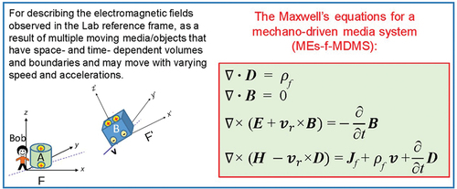
In classical electrodynamics, by motion, it always means a relative movement of two observers in inertia reference frames, so that the covariance of the Maxwell’s equations is preserved respectively in two spaces under Lorentz transformation. The energy is thus conservative for the electromagnetic system. The theory for describing the electromagnetic behavior of the charged particles in vacuum space can be well described using the special relativity because of the invariance of the speed of light in vacuum. However, for engineering applications, the media have shapes and sizes and may move with acceleration, and a system may have multiple moving objects that may be correlated or independently under external mechanical triggering. This paper presents the theory for describing the electromagnetic phenomena in this electro-magnetic-mechano system. We mainly introduce the Maxwell’s equations for a mechano-driven media system (MEs-f-MDMS) under low-speed approximation (v << c). We concluded that the MEs-f-MDMS are required for describing the electrodynamics inside a moving object that moves not only with accelerated translation motion but also has rotation motion. The classical Maxwell’s equations are to describe the electrodynamics in the region where there is no local medium movement. The full solutions of the two regions satisfy the boundary conditions, so that the rotation of the object affects the electromagnetic field at vicinity. The theoretical approaches for solving the MEs-f-MDMS are also presented.

Keywords:

• Maxwell’s equations for a mechano-driven media system (MEs-f-MDMS)
• Lorentz transformation
• moving medium/object
• Wang formulation
• special relativity

MATHEMATICS SUBJECT CLASSIFICATION:

• Y-Miscellaneous Categories
• Y4-Dissertations

1. Introduction

Studying the electrodynamics of a moving medium has a long-lasting interest and importance. For a general medium that moves with a uniform speed along a straight line, it is sufficient to use the standard differential-form Maxwell′s equations (MEs) and the approximate Minkowski constitutive equations for describing its electromagnetic behavior [1–3]. Using the Lorentz transformation, the electromagnetic fields observed in a moving frame (S′) can be derived from a non-moving observer′s reference frame (S) by preserving the covariance of the MEs with the use of Lorentz transformation [3,4]. This is the standard and well-received special relativity in classical electrodynamics. Since an important parameter in the Lorentz transformation is the speed of light, which usually means the speed of light in vacuum, therefore, the special relativity is about the same electromagnetic phenomenon observed by two independent observers located in two inertial reference frames that have a relative movement at a constant speed, and the entire space is either vacuum or filled with one type of isotropic medium without boundary. An observer named Alice is in a moving inertial frame S′ that moves at a velocity $v_0$ relative to the non-moving frame S (Lab frame). If there is a point charge +q that is at rest in the S frame, what Bob in the rest inertial frame S observes is only a Coulomb field. While for Alice, the point charge is moving at a relative velocity of –$v_0$, so that she will detect not only an electric field but also a magnetic field as caused by the moving charge +q. The magnetic field and electric field observed by Alice (B′, E′), and that by Bob (B, E) are correlated by the Lorentz transformation under the assumption of the covariance of the Maxwell’s equations.

To calculate the electromagnetic fields of a moving medium, one must have the constitutive relations of materials that are treated as supplemental conditions to solve the MEs in matter. Minkowski’s views are grounded on an assumption that the properties of the medium and the corresponding constitution equations in the rest inertial frame remain the same. There are two requirements: moving with uniform speed along a straight line or movement occurring in inertial reference frame, and the corresponding constitution equations being pre-determined in advance [3]. However, if the medium moves along a complex trajectory with acceleration (Figure 1b), and the velocity could be a function of time and position for shape-deformable materials or liquid, it would be mathematically impossible to describe the electromagnetic fields of the moving medium in this case. More importantly, practical media/materials could be anisotropic with their permittivity strongly depends on frequency and even crystal orientations, thus, the medium dispersion relationship should be considered [5]. Such cases occur a lot in engineering applications for practical materials.

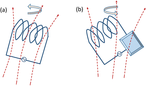
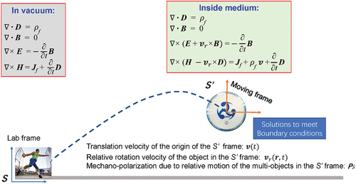
Figure 1. Two approaches for dealing with the electrodynamics of moving medium. (a) Special relativity theory is about the experience of two independent observers, Bob and Alice, who are located in different reference frames (Lab frame S, Moving frame S’) that are relatively moving at a constant velocity and along a straight line. Bob and Alice observe the same electromagnetic phenomenon occurring in vacuum space, but with different measurement results. Such an approach is most effective for describing the electrodynamics in the universe. (b) Maxwell’s equations for a mechano-driven media system (MEs-f-MDMS) is about one observer who is observing two electromagnetic phenomena, which are associated with two moving objects/media located in the two reference frames that may relatively move at v << c. In general, the media/objects have sizes and boundaries, and they may move with acceleration along complex trajectories as driven by an external force. Such theory is most effective for engineering applications, but it can go beyond. We need to point out that special relativity may not be easily adopted for describing the case shown in (b) due to the change in speed of light across medium boundary.

2. Galilean space and time

In general, there are two fundamental approaches for developing the electrodynamics of a moving medium (Figure 1). The first method is through Einstein’s relativity and Minkowski constitutive equations, forming the basis of field theory [3,6]. The relativity approach works extremely well for describing the electromagnetic behavior in vacuum, especially for universe, in which all of the stars are treated as ‘points’ without boundaries and volumes. The second approach is based on Galilean transformation, in which the space and time are independent [7,8]. So, there exists an absolute space and all inertial frames share a universal time, which are essentially different from special relativity, but it works well for engineering applications. Here, we explore the conditions under which the two approaches give the same results.

Special relativity is most powerful for treating the electromagnetic behavior observed in the Lab frame (at rest) $\left(\mathit{r},\mathit{t}\right)$ (E, B, D, H) and the moving frame affixed to the medium $({\mathit{r}}^{\mathit{\prime }},t^{\mathit{\prime }})$ (${\mathit{E}}^{\mathit{\prime }}$, ${\mathit{B}}^{\mathit{\prime }}$, ${\mathit{D}}^{\mathit{\prime }}$, ${\mathit{H}}^{\mathit{\prime }}$) that is moving at a constant velocity $v_0$ along the x-axis, which are correlated by the Lorentz transformation (Figure 2a).

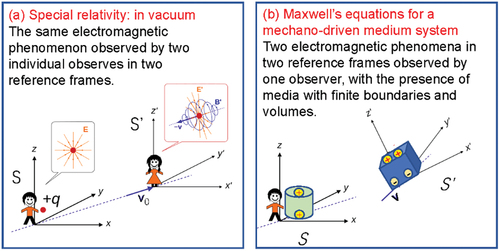
Figure 2. (a) Case for special relativity: Schematic diagram representing the general approach in special relativity, in which the fields observed by an observer who is moving at a constant velocity v about the fields (${\mathbf{\text{E}}}^{\mathit{\prime }}$, ${\mathbf{\text{B}}}^{\mathit{\prime }}$) that was first generated in the Lab frame (E, B). The Lorentz transformed relationships between the fields in the two reference frame in parallel to $\mathit{v}$ and perpendicular to v are inset. (b) Mechano-driven moving media system in non-inertia frame: A general case in which the observer is on the ground frame (called Lab frame), with several media moving at complex velocities along various trajectories as represented by the dashed lines. The medium can translate, rotate, expand and even split. The co-moving frames for the media are: (x₁, y₁, z₁), (x₂, y₂, z₂). in such a case, the Lorentz transformation for special relativity cannot be easily applied, and the only realistic approach is to express all of the fields in the frame where the observation is done (Lab frame) and all of the fields are expressed in the variables in the Lab frame.

(1a) $\mathit{x\prime }=\mathit{\gamma }\left(\mathit{x}-v_0\mathit{t}\right)$(1a)

(1b) $\mathit{y\prime }=\mathit{y}$(1b)

(1c) $\mathit{z}\mathit{\prime }=\mathit{z}$(1c)

(1d) $\mathit{t\prime }=\mathit{\gamma }(\mathit{t}-\mathit{x}{\nu }_0/c^2)$(1d)

Or equivalently:

(1e) $\frac{\partial }{\mathit{\partial t\prime }}=\mathit{\gamma }(\frac{\partial }{\mathit{\partial t}}+v_0\frac{\partial }{\mathit{\partial x}})$(1e)

(1f) $\frac{\partial }{\partial x^{\prime }}=\mathit{\gamma }(\frac{\partial }{\mathit{\partial x}}+v_0/c^2\frac{\partial }{\mathit{\partial t}})$(1f)

(1g) $\frac{\partial }{\mathit{\partial }{\mathit{y}}^{\mathit{\prime }}}=\frac{\partial }{\mathit{\partial y}}$(1g)

(1h) $\frac{\partial }{\mathit{\partial }{\mathit{z}}^{\mathit{\prime }}}=\frac{\partial }{\mathit{\partial z}}$(1h)

where $\mathit{\gamma }=1/{(1-v_0^2/c^2)}^{1/2}$, and c is the speed of light in vacuum. In the relativistic theory, space and time are unified and correlated. By assuming the covariance of the MEs and use the Lorentz transformation as stated in Equation (1a(1a) $\mathit{x\prime }=\mathit{\gamma }\left(\mathit{x}-v_0\mathit{t}\right)$(1a) –1h(1h) $\frac{\partial }{\mathit{\partial }{\mathit{z}}^{\mathit{\prime }}}=\frac{\partial }{\mathit{\partial z}}$(1h) ), the relationship between the fields observed in a moving frame in the term of those in the Lab frame can be correlated by following relationship for the fields in

(2a) ${\mathit{E}}_{//}^{\mathit{\prime }}={\mathit{E}}_{//},{\mathit{B}}_{//}^{\mathit{\prime }}={\mathit{B}}_{//},D_{//}^{\mathit{\prime }}={\mathit{D}}_{//},{\mathit{H}}_{//}^{\mathit{\prime }}={\mathit{H}}_{//},$(2a)

(2b) ${\mathit{E}}_{\mathit{\text{⟂}}}^{\prime }=\mathit{\gamma }(\mathit{E}+{\mathit{v}}_0\times \mathit{B}{)}_{\mathit{\text{⟂}}}$(2b)

(2c) ${\mathit{B}}_{\mathit{\text{⟂}}}^{\prime }=\mathit{\gamma }(\mathit{B}-{\mathit{v}}_0\times \mathit{E}/c^2{)}_{\mathit{\text{⟂}}}$(2c)

(2d) ${\mathit{D}}_{\mathit{\text{⟂}}}^{\prime }=\mathit{\gamma }(\mathit{D}+{\mathit{v}}_0\times \mathit{H}/c^2{)}_{\mathit{\text{⟂}}}$(2d)

(2e) ${\mathit{H}}_{\mathit{\text{⟂}}}^{\prime }=\mathit{\gamma }{(\mathit{H}-{\mathit{v}}_0\times \mathit{D})}_{\mathit{\text{⟂}}}$(2e)

For the purpose of our discussion, we now consider the results for low moving speed case, $v_0\ll \mathit{c}$, the fields in the two reference frames are related approximately by [9]:

(3a) ${\mathit{E}}^{\mathit{\prime }}\approx \mathit{E}+{\mathit{v}}_0\times \mathit{B}$(3a)

(3b) ${\mathit{B}}^{\mathit{\prime }}\approx \mathit{B}-{\mathit{v}}_0\times \mathit{E}/c^2$(3b)

(3c) ${\mathit{D}}^{\mathit{\prime }}\approx \mathit{D}+{\mathit{v}}_0\times \mathit{H}/c^2$(3c)

(3d) ${\mathit{H}}^{\mathit{\prime }}\approx \mathit{H}-{\mathit{v}}_0\times \mathit{D}$(3d)

(3e) ${\mathit{J}}_{\mathit{f}\mathit{\prime }}\approx \mathit{J}-\mathit{\rho }{\mathit{v}}_0$(3e)

(3f) $\mathit{\rho }\mathit{\prime }\approx \mathit{\rho }-{\mathit{v}}_0\cdot \mathit{J}/c^2$(3f)

In the Galilean transformation:

(4a) $\mathit{x}\mathit{\prime }=\mathit{x}-v_0\mathit{t}$(4a)

(4b) $\mathit{y}\mathit{\prime }=\mathit{y}$(4b)

(4c) $\mathit{z}\mathit{\prime }=\mathit{z}$(4c)

(4d) $t^{\mathit{\prime }}=\mathit{t}$(4d)

where the space and time are absolutely independent. Galilean space and time are most frequently used in classical physics and engineering applications. The fields in the two reference frames are related by:

(5a) ${\mathit{E}}^{\mathit{\prime }}=\mathit{E}+{\mathit{v}}_0\times \mathit{B}$(5a)

(5b) ${\mathit{B}}^{\mathit{\prime }}=\mathit{B}$(5b)

(5c) ${\mathit{D}}^{\mathit{\prime }}=\mathit{D}$(5c)

(5d) ${\mathit{H}}^{\mathit{\prime }}=\mathit{H}-{\mathit{v}}_0\times \mathit{D}$(5d)

(5e) ${\mathit{J}}^{\mathit{\prime }}=\mathit{J}-\mathit{\rho }{\mathit{v}}_0$(5e)

(5f) $\mathit{\rho }\mathit{\prime }=\mathit{\rho }$(5f)

The results for Galilean transformation (Equation (5a–5e) are the same as that from Lorentz transformation (Equations (3a–3d)) if $v_0\ll \mathit{c}$. This means that the electromagnetic behavior of slow-moving objects can be effectively described in the Galilean transformation. This is the case that we care about for engineering applications, as shown in Figure 2b.

The conditions under which the results from the Lorentz transformation is equivalent to that of the Galilean transformation are as following [10]:

1. The relative speed between two inertial frames of reference is much smaller than the speed of light in vacuum: $v_0\ll \mathit{c}$, so $\mathit{\gamma }\approx 1$; and

2. Galilean phenomenon takes place in an arena, the spatial extension of which is much smaller than the distance traveled by light during the duration of the phenomenon: $\mathit{x}\ll \mathit{ct}$. This condition can be understood based on following discussion. From Equation (1)(1a) $\mathit{x\prime }=\mathit{\gamma }\left(\mathit{x}-v_0\mathit{t}\right)$(1a) , under the approximation of $v_0\ll \mathit{c}$, the Lorentz transformation for time becomes $t^{\mathit{\prime }}\approx (\mathit{t}-\frac{x{v}_0}{c^2})=\frac{1}{c}(\mathit{ct}-\mathit{x}\frac{v_0}{\mathit{c}})$. If $\mathit{x}\ll \mathit{ct}$, the space caused correction to time is so small and it can completely ignored, resulting $t^{\mathit{\prime }}\approx \mathit{t}$, which is the result of Galilean transformation.

These two conditions warrant the applications of treating electromagnetic phenomena in practical engineering using Galilean transformation, so that the complication introduced by Lorentz transformation can be avoided.

3. Galilean electromagnetism

The classical MEs satisfy the covariance under Lorentz transformation, which is the foundation for correlating the electromagnetic fields observed in a moving frame S′ with that observed in the Lab frame for motions without acceleration. In the inertia reference frame, there is no external input force, so that the total electromagnetic energy is conserved. For engineering applications, approximated methods are always effective for treating practical electromagnetism in the most feasible approach. As a result, Galilean electromagnetism has been developed based on the work by Le Belllac and Levy-Léblond in 1975 [7] for describing the electromagnetic phenomenon of charged medium moving at nonrelativistic speeds. According to Rousseaux: Galilean electromagnetism is not an alternative to special relativity but is precisely its low-velocity limit in classical electromagnetism [8]. Galilean electromagnetics mainly includes two quasi-static limits of MEs: the magneto-quasi-static (MQS) limit which neglects the displacement current, and the electro-quasi-static (EQS) limit which ignores the magnetic induction. The former is a space-like limit with E$\ll$cB, while the latter is a time-like limit with E$\gg$cB. We now present the theoretical schemes of the two limit cases.

3.2.1. Electric limit

In the first case, if E$\gg$cB, one can ignore the $\frac{\partial }{\mathit{\partial t}}\mathit{B}$ term in Faraday’s law in MEs, because the time variation of the small magnetic field does not produce much electric field. Using the subscript ‘e’ to represent this case, the MEs are approximated as:

(6a) $\mathrm{\nabla }\cdot {\mathit{D}}_{\mathrm{e}}=\mathit{\rho }$(6a)

(6b) $\mathrm{\nabla }\cdot {\mathit{B}}_e=0$(6b)

(6c) $\mathrm{\nabla }\times {\mathit{E}}_e\approx 0$(6c)

(6d) $\mathrm{\nabla }\times {\mathit{H}}_e=\mathit{J}+\frac{\partial }{\mathit{\partial t}}{\mathit{D}}_{\mathrm{e}}$(6d)

The law of conservation of charges becomes:

(6e) $\mathrm{\nabla }\cdot \mathit{J}+\frac{\partial }{\mathit{\partial t}}\mathit{\rho }=0$(6e)

In Galilean transformation, we have the following operations:

(7a) $\frac{\partial }{\mathit{\partial t}\mathit{\prime }}=\frac{\partial }{\mathit{\partial t}}+{\mathit{v}}_0\cdot \mathrm{\nabla }$(7a)

(7b) $\mathrm{\nabla }\mathit{\prime }=\mathrm{\nabla }$(7b)

Using which, we can prove that Equations (6a–6d) are covariant under the Galilean transformation, and the corresponding fields in the two reference frames are correlated by:

(8a) ${\mathit{E}}_e^{\mathit{\prime }}\approx {\mathit{E}}_e$(8a)

(8b) ${\mathit{B}}_e^{\mathit{\prime }}\approx {\mathit{B}}_e-{\mathit{v}}_0\times {\mathit{E}}_e/c^2$(8b)

(8c) ${\mathit{D}}_e^{\mathit{\prime }}\approx {\mathit{D}}_e$(8c)

(8d) ${\mathit{H}}_e^{\mathit{\prime }}\approx {\mathit{H}}_e-{\mathit{v}}_0\times {\mathit{D}}_e$(8d)

(8e) ${\mathit{J}}^{\mathit{\prime }}\approx \mathit{J}-\mathit{\rho }{\mathit{v}}_0$(8e)

(8f) ${\rho }^{\mathit{\prime }}\approx \mathit{\rho }$(8f)

which are just the result from the Lorentz transformation under the approximations of E$\gg$cB and $v_0\ll$c.

3.2.2. Magnetic limit

In the first case, if E$\ll$cB, one can ignore the ${\displaystyle \frac{\partial }{\mathit{\partial t}}{\mathit{D}}^{\mathit{\prime }}}$ term in Ampere’s law in MEs, because the small displacement current does not produce a significant magnetic field. Using the subscript m to represent this case, we have:

(9a) $\mathrm{\nabla }\cdot {\mathit{D}}_m=\mathit{\rho }$(9a)

(9b) $\mathrm{\nabla }\cdot {\mathit{B}}_m=0$(9b)

(9c) $\mathrm{\nabla }\times {\mathit{E}}_m=-\frac{\partial }{\mathit{\partial t}}{\mathit{B}}_m$(9c)

(9d) $\mathrm{\nabla }\times {\mathit{H}}_m\approx \mathit{J}$(9d)

The law of the conservation of charges becomes:

(9e) $\mathrm{\nabla }\cdot \mathit{J}=0$(9e)

Physically, the theory based on these equations will describe situations where the electric current is the dominant source of electromagnetic behavior. Accordingly, from Equations (3a–3f), the fields in the moving frame S′ and that in Lab frame S are correlated by:

(10a) ${\mathit{E}}_m^{\mathit{\prime }}\approx {\mathit{E}}_m+{\mathit{v}}_0\times {\mathit{B}}_m$(10a)

(10b) ${\mathit{B}}_m^{\mathit{\prime }}\approx {\mathit{B}}_m$(10b)

(10c) ${\mathit{D}}_m^{\mathit{\prime }}\approx {\mathit{D}}_m+{\mathit{v}}_0\times \mathit{H}/c^2$(10c)

(10d) ${\mathit{H}}_m^{\mathit{\prime }}\approx {\mathit{H}}_m$(10d)

(10e) ${\mathit{J}}^{\mathit{\prime }}\approx \mathit{J}$(10e)

(10f) ${\rho }^{\mathit{\prime }}\approx \mathit{\rho }-{\mathit{v}}_0\cdot \mathit{J}/c^2$(10f)

One can prove that Equations (8a(8a) ${\mathit{E}}_e^{\mathit{\prime }}\approx {\mathit{E}}_e$(8a) –8d(8d) ${\mathit{H}}_e^{\mathit{\prime }}\approx {\mathit{H}}_e-{\mathit{v}}_0\times {\mathit{D}}_e$(8d) ) and (10a(10a) ${\mathit{E}}_m^{\mathit{\prime }}\approx {\mathit{E}}_m+{\mathit{v}}_0\times {\mathit{B}}_m$(10a) –10c(10c) ${\mathit{D}}_m^{\mathit{\prime }}\approx {\mathit{D}}_m+{\mathit{v}}_0\times \mathit{H}/c^2$(10c) ) satisfy the Galilean covariance.

The two limiting cases shown in this section satisfy the Galilean covariance, and the results are very useful for dealing with many electromagnetic phenomena in engineering, and they have been very useful for many cases. For a general case in which the approximations we made above may not be valid if one considers the relative strengths of the fields, a more general theory is thus required.

4. Faraday’s law for a moving object

The general equation for the Faraday’s law is for stationary medium with only considering the time-dependent behavior of the electromagnetic field. We now start from the physics principle to derive the equation for a moving medium/object, instead of from equations to equations. The mathematical expression of the Faraday’s law of electromagnetic induction is the Lentz’s flux-rule: the reducing rate of the magnetic flux is the electromotive force (EMF):

(11) ${\xi }_{\mathit{EMF}}=-\frac{\mathit{d}{\mathit{\Phi }}_{\mathit{B}}}{\mathit{dt}}=-\frac{d}{\mathit{dt}}{\iint }_{\mathit{s}(\mathit{t})}\mathit{B}\cdot \mathit{d}\mathit{s}$(11)

where the integral is over an open surface s(t) whose shape and open edge could be time-dependent, which represents a moving object with deformable shape. Equation (11)(11) ${\xi }_{\mathit{EMF}}=-\frac{\mathit{d}{\mathit{\Phi }}_{\mathit{B}}}{\mathit{dt}}=-\frac{d}{\mathit{dt}}{\iint }_{\mathit{s}(\mathit{t})}\mathit{B}\cdot \mathit{d}\mathit{s}$(11) is the flux – rule and it can be used to describe most of the electromagnetic phenomena, especially for power generation and electric motor. Figure 3a represents a general case that can be well described using the flux-rule, in which a thin-wire circuit has a fixed shape but may move as a solid translation.

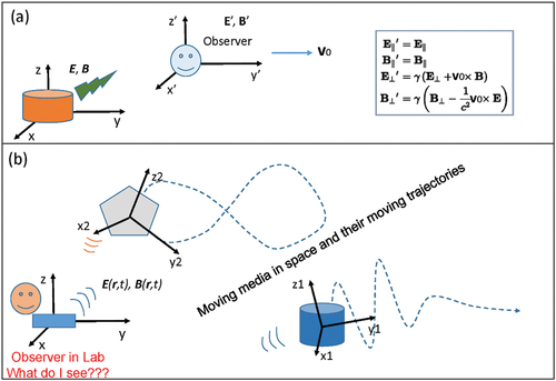
Figure 3. Several cases regarding to the flux rule for electromagnetic induction. (a): A typical example of thin wire circuit that is moving with acceleration with respect to the Lab frame in a time- and space- dependent magnetic field. (b): A conductive fan that is rotating inside a uniform magnetic field. (c) A rectangular thin wire circuit that is at stationary in a uniform magnetic field, but with one end sliding on the edge of a rotating conductive disc at t = 0 and t = t, and the other end is connected to the axis of the disc. The unit charge within the macroscopic size object can move, which leads to an additional term in the Faraday’s law for electromagnetic induction.

However, there are a few cases that appear to be ‘anti-flux-rule’, as presented by Feynman [11]. The anti-flux rule examples occur in cases that there are a large conductive piece appearing in the electric circuit that rotates around an axis, such as the two cases shown in Figures 3b,c, which has been referred as one-piece Faraday generator [12,13]. A common characteristic of the ‘anti-flux’ examples is that the circuit contains a large-size metal piece, in which the moving trajectory of a point charge depends on the force acting on it besides the geometrical ‘confining effect’ of the transport circuit. Take the case in Figure 3c as an example, in which a rotating metal disc is present in a magnetic field, and part of the circuit is a sliding needle at its edge. Once the disc rotates, the total magnetic flux goes through the circuit may not change, so that there would be no EMF according to Equation (11)(11) ${\xi }_{\mathit{EMF}}=-\frac{\mathit{d}{\mathit{\Phi }}_{\mathit{B}}}{\mathit{dt}}=-\frac{d}{\mathit{dt}}{\iint }_{\mathit{s}(\mathit{t})}\mathit{B}\cdot \mathit{d}\mathit{s}$(11) , but the EMF does exist experimentally! This paradox was not clearly explained by Feynman. In his text book, he said ‘It must be applied to circuits in which the material of the circuit remains the same. When the material of the circuit is changing, we must return to the basic laws. The correct physics is always given by the two basic laws $\mathrm{\nabla }\times \mathit{E}=-\frac{\partial }{\mathit{\partial t}}\mathit{B}$, F = q(E + v×B).’ [11]. It appears that such examples were not clearly explained by Feynman. Here the addition of Lorentz force is to make up the shortcoming of the MEs in treating the electromagnetic behavior of moving object. Therefore, we now present more detailed discussions about this case.

The ‘anti-flux-rule’ case is likely due to that the path of a unit charge moving in the disc (as indicated by a blue dashed line) deviates from the original rectangular ‘circuit’ (as indicated by black dashed line in Figure 3c,l), along which the integral for calculating the magnetic flux is done [14]. As the charge enters the disc at point P₁ at its edge at t = 0, it moves along the radial direction to point P₂ as the disc rotates to t = t; its moving path is indicated by a blue dashed line. Therefore, the area as defined by the two dashed lines in Figure 6cIIb is the effective area of change of magnetic flux. This change in flux is due to the deviation of the unit charge transport path from that of the geometrical path as the disc rotates. This is caused by the existence of the large metal disc in the circuit, and the rotation of which produces the observed EMF. To include this argument officially in the equation, we firstly focus on the expansion of the Faraday’s law.

To carry on the mathematical calculation in Equation (11)(11) ${\xi }_{\mathit{EMF}}=-\frac{\mathit{d}{\mathit{\Phi }}_{\mathit{B}}}{\mathit{dt}}=-\frac{d}{\mathit{dt}}{\iint }_{\mathit{s}(\mathit{t})}\mathit{B}\cdot \mathit{d}\mathit{s}$(11) , we use a flux theorem (see [15]): for a general functions G(r,t), the boundary surface of which moves at a velocity field $\mathit{v}\left(\mathit{r},\mathit{t}\right)$ [16], we have

(12) $\frac{\mathit{d}}{\mathit{d}t}\iint \mathit{C}\mathit{G}\cdot \mathit{\text{d}}\mathit{s}=\iint \mathit{C}[\frac{\partial }{\mathit{\partial t}}\mathit{G}+(\mathit{G}\cdot \mathrm{\nabla }\text{)}\mathit{v}+\left(\mathrm{\nabla }\cdot \mathit{G}\right)\mathit{v}-\left(\mathrm{\nabla }\cdot \mathit{v}\text{)}\mathit{G}\right]\cdot \mathit{\text{d}}\mathit{s}-\underset{C}{\oint }\left(\mathit{v}\times \mathit{G}\right)\mathit{\text{d}}\mathit{L}$(12)

Using this mathematical identity, Equation (11)(11) ${\xi }_{\mathit{EMF}}=-\frac{\mathit{d}{\mathit{\Phi }}_{\mathit{B}}}{\mathit{dt}}=-\frac{d}{\mathit{dt}}{\iint }_{\mathit{s}(\mathit{t})}\mathit{B}\cdot \mathit{d}\mathit{s}$(11) becomes [17]:

(13) ${\xi }_{\text{EMF}}=-\frac{d}{\mathit{dt}}{\iint }_{\mathit{s}(\mathit{t})}\mathit{B}\cdot \mathit{d}\mathit{s}\mathbf{=}-{\iint }_{\mathbf{s}(t)}\{\frac{\partial }{\mathit{\partial t}}\mathit{B}-\mathrm{\nabla }\times [\mathit{v}\times \mathit{B}]\}\cdot \mathit{d}\mathit{s}$(13)

where $\mathit{v}$ is the velocity at which the boundary surface moves. More general discussion has been given by Scanlon et al. [18]. Equation (11)(11) ${\xi }_{\mathit{EMF}}=-\frac{\mathit{d}{\mathit{\Phi }}_{\mathit{B}}}{\mathit{dt}}=-\frac{d}{\mathit{dt}}{\iint }_{\mathit{s}(\mathit{t})}\mathit{B}\cdot \mathit{d}\mathit{s}$(11) and Equation (11)(11) ${\xi }_{\mathit{EMF}}=-\frac{\mathit{d}{\mathit{\Phi }}_{\mathit{B}}}{\mathit{dt}}=-\frac{d}{\mathit{dt}}{\iint }_{\mathit{s}(\mathit{t})}\mathit{B}\cdot \mathit{d}\mathit{s}$(11) applies to the case that there is no change of the closed circuit, for instance, there is no relative sliding between the wire and the disc, such as in Figure 3a. While in Equation (13)(13) ${\xi }_{\text{EMF}}=-\frac{d}{\mathit{dt}}{\iint }_{\mathit{s}(\mathit{t})}\mathit{B}\cdot \mathit{d}\mathit{s}\mathbf{=}-{\iint }_{\mathbf{s}(t)}\{\frac{\partial }{\mathit{\partial t}}\mathit{B}-\mathrm{\nabla }\times [\mathit{v}\times \mathit{B}]\}\cdot \mathit{d}\mathit{s}$(13) , $\mathit{v}$ means the moving velocity of the circuit, and it allows a flexible or changeable contact between the wire and the disc. Most importantly, if the circuit is not a closed loop as in Figure 3b, Equation (13)(13) ${\xi }_{\text{EMF}}=-\frac{d}{\mathit{dt}}{\iint }_{\mathit{s}(\mathit{t})}\mathit{B}\cdot \mathit{d}\mathit{s}\mathbf{=}-{\iint }_{\mathbf{s}(t)}\{\frac{\partial }{\mathit{\partial t}}\mathit{B}-\mathrm{\nabla }\times [\mathit{v}\times \mathit{B}]\}\cdot \mathit{d}\mathit{s}$(13) should be used [19].

For the cases shown in Figures 3b,c, where the total flux does not change as the fan is rotating in a uniform magnetic field just based on the size of the geometrical area, but there is a potential drop generated along the fan blade due to the Lorentz force (e.g. motion generated potential) [20]. This is because the effective area swiped across by the fan blade as the unit charge travels along the fan blade, which causes a change in magnetic flux. As the fan rotates, the work done by the Lorentz force on the unit charge according to Equation (13)(13) ${\xi }_{\text{EMF}}=-\frac{d}{\mathit{dt}}{\iint }_{\mathit{s}(\mathit{t})}\mathit{B}\cdot \mathit{d}\mathit{s}\mathbf{=}-{\iint }_{\mathbf{s}(t)}\{\frac{\partial }{\mathit{\partial t}}\mathit{B}-\mathrm{\nabla }\times [\mathit{v}\times \mathit{B}]\}\cdot \mathit{d}\mathit{s}$(13) is: ${\xi }_{\text{EMF}}={\int }_0^a\mathit{r\omega }{B}_{\text{0}}\mathit{dr}=\frac{1}{2}\mathit{\omega }{a}^2{B}_0$.

For the case shown in Figure 3cII, the charge can move inside the conductive disc at a velocity of $v_r=\mathit{r\omega }$ perpendicular to the radial direction, where $\mathit{\omega }$is the angular velocity, thus the total electromotive force is along the entire radius a from P₁ to O, with a potential drop calculated using Lorentz force: ξ_EMF = $\underset{a}{\overset{0}{\int }}\left[{\mathit{v}}_r\times \mathit{B}\right]\cdot \text{d}\mathit{r}$= $\underset{0}{\overset{a}{\int }}\mathit{r\omega }{B}_0\mathit{dr}=\frac{1}{2}\mathit{\omega }{a}^2{B}_0,$and the current flowing in the circuit is $\frac{1}{2\mathit{R}}\mathit{\omega }{a}^2{B}_0$.

Alternatively, using the flux rule (Equation 10(10a) ${\mathit{E}}_m^{\mathit{\prime }}\approx {\mathit{E}}_m+{\mathit{v}}_0\times {\mathit{B}}_m$(10a) ), the area of the disc segment between the two dashed lines is: $\mathit{A}=\frac{1}{2}\mathit{\omega t}{a}^2$, so ξ_EMF = A$B_0/\mathit{t}$ =$\frac{1}{2}\mathit{\omega }{a}^2{B}_0$. The results are equivalent to that received using Lorentz force [14].

Therefore, the examples of the ‘anti-flux’ are likely due to that the path of the unit charge moving in the disc (blue dashed line) deviates from the original rectangular ‘circuit’ (as indicated by black dashed line in Figure 3c), along which the integral for calculating the magnetic flux is done. As the charge enters the disc at point P₁ at its edge at t = 0, it moves along the radial to point P₂ as the disc rotates at t = t (Figure 3c); its moving path is indicated by a blue dashed line. Therefore, the area as defined by the two dashed lines in Figure 3c is the effective area of change of magnetic flux. This change in flux is due to the deviation of the unit charge transport path from that of the geometrical path as the disc rotates. Therefore, the understanding of flux rule needs to consider the charge transport process if there is a relative movement in the conductive medium and a change in circuit structure, such as sliding.

The example illustrated in Figure 3c is a great example regarding to electrodynamics of a moving media system. The thin wire section is at stationary, but the metal disc is rotating, with a needle sliding on it edge. The moving velocities of the space points inside the disc are space (r)- and time-dependent, and there is acceleration during disc rotation. This is a good example of why we have to expand the Maxwell’s equations for a moving media system.

Now we derive the Faraday’s law in differential form starting from its integral form with considering the movement of object/medium [21]:

(14) ${\oint }_C{\mathit{E}}^{\mathit{\prime }}\cdot \mathit{d}\mathit{L}=-\frac{d}{\mathit{dt}}{\iint }_{\mathit{s}(\mathit{t})}\mathit{B}\cdot \mathit{d}\mathit{s}$(14)

where E′ represents the electric field in the rest frame of each segment dL of the path of integration. The Faraday’s law means that the reducing rate of the magnetic flux through an open surface is the circulation of the electric field around its looped edge. We now need to express $\mathit{E}\mathit{\prime }$in the terms of the field E and B in Lab frame. Using Equation (12)(12) $\frac{\mathit{d}}{\mathit{d}t}\iint \mathit{C}\mathit{G}\cdot \mathit{\text{d}}\mathit{s}=\iint \mathit{C}[\frac{\partial }{\mathit{\partial t}}\mathit{G}+(\mathit{G}\cdot \mathrm{\nabla }\text{)}\mathit{v}+\left(\mathrm{\nabla }\cdot \mathit{G}\right)\mathit{v}-\left(\mathrm{\nabla }\cdot \mathit{v}\text{)}\mathit{G}\right]\cdot \mathit{\text{d}}\mathit{s}-\underset{C}{\oint }\left(\mathit{v}\times \mathit{G}\right)\mathit{\text{d}}\mathit{L}$(12) , Equation (14)(14) ${\oint }_C{\mathit{E}}^{\mathit{\prime }}\cdot \mathit{d}\mathit{L}=-\frac{d}{\mathit{dt}}{\iint }_{\mathit{s}(\mathit{t})}\mathit{B}\cdot \mathit{d}\mathit{s}$(14) becomes:

(15) ${\oint }_C({\mathit{E}}^{\mathit{\prime }}\mathbf{-}\mathit{v}\mathbf{\times }\mathit{B})\cdot \mathit{d}\mathit{L}=-{\iint }_{\mathit{s}(\mathit{t})}\frac{\partial }{\mathit{\partial t}}\mathit{B}\cdot \mathit{d}\mathit{s}$(15)

The Lorentz force acting on a point charge q in the observer Bob’s frame is F = q ($\mathit{E}+{\mathit{v}}_t\times \mathit{B}$), where ${\mathit{v}}_t$is the total moving velocity of the point charge that may be different from the moving velocity $\mathit{v}$ of the circuit. Alternatively, the force acting on the same charge in its rest frame is $\mathit{F}\mathit{\prime }$ = q$\mathit{E}\mathit{\prime }$. In general, F ≠ $\mathit{F}\mathit{\prime }$ because of the accelerated movement of the circuitry surface boundary, unless the moving frame is an inertia frame [22], which means that we must have $\mathit{v}={\mathit{v}}_0.$Therefore, only when the medium movement is at a constant speed along a straight line, $\mathit{v}={\mathit{v}}_0,$ we can have $\mathit{F}\mathit{\prime }$ = q$\mathit{E}\mathit{\prime }$ for both inertia reference frames, which gives $\mathit{E}\mathit{\prime }$ = $\mathit{E}+{\mathit{v}}_t\times \mathit{B}$.

When the medium moves with an acceleration, the electromagnetic behavior of the moving medium becomes complex. We take a unit charge q as an example. If the medium that carriers the unit charge experiences an acceleration motion, the force acting on the unit charge should include the inertia force $\frac{\partial }{\mathit{\partial t}}\text{(}\mathit{\text{mv}}\text{)}$ besides the electromagnetic force, where m is the mass of the point charge. In this case, we have:

(16) $\mathit{q}\mathit{E}\mathit{\prime }-\frac{\partial }{\mathit{\partial t}}\left(\mathit{m}\mathit{v}\right)=\mathit{q}\mathit{E}+\mathit{q}{\mathit{v}}_t\times \mathit{B}$(16)

where ${\mathit{v}}_t$ is the total moving velocity of the unit charge in the S frame. ${\mathit{v}}_t$ can be split into two components for a general case: moving velocity $\mathit{v}$ of the origin of the reference frame $\mathit{S}\mathit{\prime }$, which is only time-dependent so that it can be viewed as a ‘rigid translation’, and ${\mathit{v}}_r$ is the relative moving velocity of the point charge with respect to the reference frame $\mathit{S}\mathit{\prime }$, which is space- and time-dependent

(17) ${\mathit{v}}_t=\mathit{v}\left(\mathit{t}\right)+{\mathit{v}}_r\left(\mathit{r},\mathit{t}\right)$(17)

The space dependence of ${\mathit{v}}_r$ represents the shape deformation and/or rotation of the medium, and time dependence represents the local acceleration. Substituting Equations (16)(3c) ${\mathit{D}}^{\mathit{\prime }}\approx \mathit{D}+{\mathit{v}}_0\times \mathit{H}/c^2$(3c) and (17(3d) ${\mathit{H}}^{\mathit{\prime }}\approx \mathit{H}-{\mathit{v}}_0\times \mathit{D}$(3d) ) into Equation (15)(15) ${\oint }_C({\mathit{E}}^{\mathit{\prime }}\mathbf{-}\mathit{v}\mathbf{\times }\mathit{B})\cdot \mathit{d}\mathit{L}=-{\iint }_{\mathit{s}(\mathit{t})}\frac{\partial }{\mathit{\partial t}}\mathit{B}\cdot \mathit{d}\mathit{s}$(15) , we have

(18) ${\oint }_C[\mathit{E}+{\mathit{v}}_r\mathbf{\times }\mathit{B}+\frac{1}{q}\frac{\partial }{\mathit{\partial t}}\left(\mathit{m}\mathit{v}\right)]\cdot \mathit{d}\mathit{L}=-{\iint }_s\frac{\partial }{\mathit{\partial t}}\mathit{B}\cdot \mathit{d}\mathit{s}$(18)

We now consider two cases [5,14]:

1). If the medium is a circuit that is a thin wire loop, so that the moving velocity ${\mathit{v}}_r$of a point charge inside the wire is parallel to the wire, e.g. ${\mathit{v}}_r$ is parallel to the integral path $\mathit{\text{dL}}$, the term $[{\mathit{v}}_r\times \mathit{B}]\cdot \mathit{d}\mathit{L}$ vanishes automatically [20]. In addition the motion of the reference is a solid translation so that $\mathit{v}\left(\mathit{t}\right)$ is only time-dependent, the third term in Equation (18)(18) ${\oint }_C[\mathit{E}+{\mathit{v}}_r\mathbf{\times }\mathit{B}+\frac{1}{q}\frac{\partial }{\mathit{\partial t}}\left(\mathit{m}\mathit{v}\right)]\cdot \mathit{d}\mathit{L}=-{\iint }_s\frac{\partial }{\mathit{\partial t}}\mathit{B}\cdot \mathit{d}\mathit{s}$(18) vanishes as well, resulting in the standard Maxwell’s equation. $\mathrm{\nabla }\times \mathit{E}=-\frac{\partial }{\mathit{\partial t}}\mathit{B}$. This means that the standard form of the Faraday’s law in differential form is valid for all thin-wire circuit case. This is the case presented in all of the text books, but it has a condition of thin wire approximation, which needs to be elaborated here. The thin wire circuit is an imaginary circuit whose shape is arbitrary. According to the flux rule, thin wire circuit means that the moving trajectory of the unit charge is exactly the integral path for calculating the magnetic flux, and the circuit is taken as an imaginary circuit when we convert the integral equation into differential form. If the imaginary circuit can be expanded to any space, the thin circuit assumption holds exactly if the circuit does not intercept with any conductive medium boundary, so that it is only exact for vacuum space case, but may not be applicable to the case if there is a moving macroscopic medium.

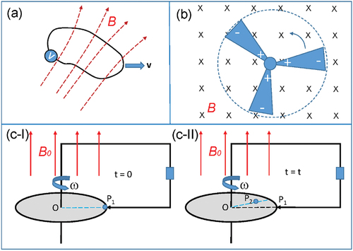
Therefore, in practice, if there are only rotating thin wires in the circuit without the presence of bulk medium on the path of electron flow, such as the case shown in Figure 4a, the MEs remain the same although the thin-wire circuit may rotate, move with acceleration, and/or have a varying shape. In this case, since the wire is so thin that there is no need to consider it as a separate medium in the calculation of electrodynamics.

Figure 4. Schematic diagram showing an accelerated moving circuit that is made of thin wires (a), and the case if there is a large bulk piece of medium incepting the circuit (b), with the presence of magnetic field.

2). The medium is large so that the relative velocity of the unit charge has a component perpendicular to the integral path in the segment where the integral loop intercepts with a conduction medium, such as the case shown in Figure 3c, such cases occur in engineering due to the size, shape and volume of the media, which cannot be ignored or taken as a point due to the space in which the electromagnetic behavior is considered.

The example in Figure 3c can be extrapolated to a general case in which $\underset{C}{\oint }\left[{\mathit{v}}_r\times \mathit{B}\right]\cdot \mathit{\text{d}}\mathit{L}$≠ 0 for the space inside the medium, because the charge moving trajectory does not coincidence with that of the integral path, so that the Lorentz force can acts on it locally although there is no change in total magnetic flux from geometrical point of view. This example also gives us an understanding about the meaning of the relative movement velocity ${\mathit{v}}_r$. Using the Stokes theorem, Equation (18)(18) ${\oint }_C[\mathit{E}+{\mathit{v}}_r\mathbf{\times }\mathit{B}+\frac{1}{q}\frac{\partial }{\mathit{\partial t}}\left(\mathit{m}\mathit{v}\right)]\cdot \mathit{d}\mathit{L}=-{\iint }_s\frac{\partial }{\mathit{\partial t}}\mathit{B}\cdot \mathit{d}\mathit{s}$(18) becomes

(19) $\mathrm{\nabla }\times [\mathit{E}+{\mathit{v}}_r\times \mathit{B}+\frac{1}{q}\frac{\partial }{\mathit{\partial t}}\left(\mathit{m}\mathit{v}\right)]=-\frac{\partial }{\mathit{\partial t}}\mathit{B}$(19)

Since the movement of the origin of the reference frame $\mathit{S}\mathit{\prime }$ that is affixed to the moving medium can be treated as a rigid translation so that it is only time-dependent, $\mathit{v}(\mathit{t}$), which means $\mathrm{\nabla }\times \left(\frac{\partial }{\mathit{\partial t}}(\mathit{m}\mathit{v}(\mathit{t}))\right)=\frac{\partial }{\mathit{\partial t}}[\mathit{m}\mathrm{\nabla }\times \mathit{v}(\mathit{t})]=0$, so that the inertia force term drops out naturally in the differential equation, we have [14]:

(20) $\mathrm{\nabla }\times (\mathit{E}+{\mathit{v}}_r\times \mathit{B})=-\frac{\partial }{\mathit{\partial t}}\mathit{B}$(20)

This case is rarely discussed in classical text books. Equation (20)(20) $\mathrm{\nabla }\times (\mathit{E}+{\mathit{v}}_r\times \mathit{B})=-\frac{\partial }{\mathit{\partial t}}\mathit{B}$(20) can be applied to cases that have a fan-blade shape rotating media and a rotation metal disc in a magnetic field as illustrated in Figures 3b,c. The finite size of the medium/circuit allows the charge to ‘wonder’ inside the conductive component, so that it is not easy to define where is the integral path of the circuit across the media.

In Equation (18)(18) ${\oint }_C[\mathit{E}+{\mathit{v}}_r\mathbf{\times }\mathit{B}+\frac{1}{q}\frac{\partial }{\mathit{\partial t}}\left(\mathit{m}\mathit{v}\right)]\cdot \mathit{d}\mathit{L}=-{\iint }_s\frac{\partial }{\mathit{\partial t}}\mathit{B}\cdot \mathit{d}\mathit{s}$(18) , when the integral path C is intercepted by a bulk size medium, inside which the practical moving velocity of the point charge may not be parallel to the integral path within the conductive medium, the term of ${\mathit{v}}_r$×B appears in the equation. It should be noticed that the relative velocity ${\mathit{v}}_r$ of the charge inside a medium may not be small in comparison to its moving velocity $\mathit{v}(\mathit{t}$) of the reference frame. This the case shown in Figure 4b.

Now let’s look at the case presented in Figure 3c. If the magnetic field is time-independent, $\frac{\partial }{\mathit{\partial t}}\mathit{B}=0$, from Equation (20)(20) $\mathrm{\nabla }\times (\mathit{E}+{\mathit{v}}_r\times \mathit{B})=-\frac{\partial }{\mathit{\partial t}}\mathit{B}$(20) , we have $\mathrm{\nabla }\times \mathit{E}=-\mathrm{\nabla }\times ({\mathit{v}}_{\mathit{\text{r}}}\times \mathit{B})$, which means that the movement of a medium in a magnetic field would generate an electric field, resulting in an electromotive force, which agrees with experimental observations. However, the situation is different if one use the classical MEs, one would have $\mathrm{\nabla }\times \mathit{E}=0$, which means E = 0, and there should be no electromotive force. This apparently disagrees with experimental observations. Such discrepancy is due to the fact that medium motion was not considered in classical MEs!

5. Ampere–Maxwell’s law for a moving object

5.2.1. Mathematical derivation

We now consider the Ampere–Macium case:

(21) ${\oint }_C{\mathit{H}}^{\mathit{\prime }}\cdot \mathit{d}\mathit{L}=\iint \mathit{s}\mathit{Jd}\mathit{s}+\frac{d}{\mathit{dt}}\iint \mathit{s}\mathit{D}\cdot \mathit{d}\mathit{s}$(21)

where the $H^{\mathit{\prime }}$ is the magnetic field on the moving medium in the frame where $\mathit{d}\mathit{L}$ is at rest. The Ampere–Maxwell’s law means that the total current through an open surface plus the increasing rate of the electric flux through an open surface is the circulation of the magnetic field around its looped edge. Using the flux theorem Equation (12)(12) $\frac{\mathit{d}}{\mathit{d}t}\iint \mathit{C}\mathit{G}\cdot \mathit{\text{d}}\mathit{s}=\iint \mathit{C}[\frac{\partial }{\mathit{\partial t}}\mathit{G}+(\mathit{G}\cdot \mathrm{\nabla }\text{)}\mathit{v}+\left(\mathrm{\nabla }\cdot \mathit{G}\right)\mathit{v}-\left(\mathrm{\nabla }\cdot \mathit{v}\text{)}\mathit{G}\right]\cdot \mathit{\text{d}}\mathit{s}-\underset{C}{\oint }\left(\mathit{v}\times \mathit{G}\right)\mathit{\text{d}}\mathit{L}$(12) , we have

(22) ${\oint }_C{\mathit{H}}^{\prime }\cdot \mathit{dL}={\iint }_s(\mathit{J}+\mathit{\rho }\mathit{v})\cdot \mathit{d}\mathit{s}+{\iint }_s\frac{\partial }{\mathit{\partial t}}\mathit{D}\cdot \mathit{d}\mathit{s}-{\oint }_C(\mathit{v}\times \mathit{D})\mathit{d}\mathit{L}$(22)

Using the Stokes theorem on the left-hand side of Equation (22)(22) ${\oint }_C{\mathit{H}}^{\prime }\cdot \mathit{dL}={\iint }_s(\mathit{J}+\mathit{\rho }\mathit{v})\cdot \mathit{d}\mathit{s}+{\iint }_s\frac{\partial }{\mathit{\partial t}}\mathit{D}\cdot \mathit{d}\mathit{s}-{\oint }_C(\mathit{v}\times \mathit{D})\mathit{d}\mathit{L}$(22) , we have

(23) $\mathrm{\nabla }\times ({\mathit{H}}^{\prime }+\mathit{v}\times \mathit{D})=\mathit{J}+\mathit{\rho }\mathit{v}+\frac{\partial }{\mathit{\partial t}}\mathit{D}$(23)

Under low speed limit, from Equation (5d)(5d) ${\mathit{H}}^{\mathit{\prime }}=\mathit{H}-{\mathit{v}}_0\times \mathit{D}$(5d) , the local magnetic field in the moving frame is

${\mathit{H}}^{\prime }\approx \mathit{H}-{\mathit{v}}_t\times \mathit{D},$

we have

(24) $\mathrm{\nabla }\times (\mathit{H}-{\mathit{v}}_r\times \mathit{D})\approx \mathit{J}+\mathit{\rho }\mathit{v}+\frac{\partial }{\mathit{\partial t}}\mathit{D}$(24)

The terms ${\mathit{v}}_r\times \mathit{D}$ is the electric field induced magnetization due to media movement. Accordingly, it is possible to produce the same magnetic field either by a conduction current, or by the motion of a charged body, or by ther motion of a polarized body.

5.2.2. Explanations of the Röntgen and Eichenwald experiments

We now consider a simple case in which the electric field is a constant, $\frac{\partial }{\mathit{\partial t}}\mathit{D}=0$, and there are no external current or charges, Equation (24)(24) $\mathrm{\nabla }\times (\mathit{H}-{\mathit{v}}_r\times \mathit{D})\approx \mathit{J}+\mathit{\rho }\mathit{v}+\frac{\partial }{\mathit{\partial t}}\mathit{D}$(24) gives, $\mathrm{\nabla }\times \mathit{H}\approx \mathrm{\nabla }\times \text{(}{\mathit{v}}_r\times \mathit{D}\text{)}$. This means that a magnetic field $\mathit{H}\approx {\mathit{v}}_r\times \mathit{D}$ would be generated if a medium is rotating inside an electric field. This is the results of the Röntgen and Eichenwald experiments, as shown in Figure 5 [23]. Such experiments are usually listed in the description of special relativity. In our opinion, they have no relationship with special relavitity since the moving velocity is extremely low, instead they are the result of the electromagnetism of moving objects/medium described by Equation (24)(24) $\mathrm{\nabla }\times (\mathit{H}-{\mathit{v}}_r\times \mathit{D})\approx \mathit{J}+\mathit{\rho }\mathit{v}+\frac{\partial }{\mathit{\partial t}}\mathit{D}$(24) .

Figure 5. (a) Set up of the Röntgen and Eichenwald experiments. (b) Measurement of the convention current ($\mathit{\rho }\mathit{v}$) that produces the same magnetic field as in (a). (c) Method of measuring the magnetic field produced by a polarization current represented by [$\mathrm{\nabla }\times ({\mathit{v}}_r\times \mathit{D})+\frac{\partial }{\mathit{\partial t}}\mathit{D}]$. Reproduced with permission from Dover Publications [23].

A circular hard rubber disc of thickness d is mounted on bearings so as to be free to rotate about a vertical axis, as shown in Figure 5a. Attached rigidly to it above and below are metal rings of radial width b. Each metal ring has been cut right through at one place by a narrow radial slit. The two metal rings are connected to the terminals of a voltage source and thus become charged to a potential difference V. The apparatus including the rubber disc and the metal rings may now be set in rotation motion as a single solid piece (the Rowland experiment), In any case, we have the following charges with which to reckon: true surface charges on the metal plates: σ₁ = εV/d; surface charges on the hard rubber disc: σ₂ = − (ε −1)V/d. If both disc and rings be placed in rotation, the upper metal ring carries a convection current vbσ₁ along the ring, where v is the linear rotation speed of the ring, and the adjacent surface of the hard rubber carries the current vbσ₂. In all, then, we have a convection current of vb (σ₁ +σ₂) = vbV/d. This current is represented by the second term at the right-hand side of Equation (24)(24) $\mathrm{\nabla }\times (\mathit{H}-{\mathit{v}}_r\times \mathit{D})\approx \mathit{J}+\mathit{\rho }\mathit{v}+\frac{\partial }{\mathit{\partial t}}\mathit{D}$(24) .

Alternatively, if the metal rings as shown in Figure 5a are unattached to the rubber disc, and the rotation is applied only to the rubber disc and the metal rings are at rest (the Röntgen experiment), and the connection of circuit is shown in Figure 5b. In this case, the convection current is only generated by the motion of the charges on the rubber disc surface, which is -vb(ε −1)V/d.

Furthermore, the correction to the local magnetic field arising from the motion of polarized medium is represented by the second term $-\mathrm{\nabla }\times \text{(}{\mathit{v}}_r\times \mathit{D}\text{)}$ in Equation (24)(24) $\mathrm{\nabla }\times (\mathit{H}-{\mathit{v}}_r\times \mathit{D})\approx \mathit{J}+\mathit{\rho }\mathit{v}+\frac{\partial }{\mathit{\partial t}}\mathit{D}$(24) . In the apparatus shown in Figure 5c, there is a rotating hard-rubber disc. It moves between two stationary and unattached metal rings, the upper of which is made up of two semicircular halves. The low ring is grounded while the two upper halves are connected to equal but opposite sources of an electric potential, +V, and –V. A dedicated pivoted magnetized needle free to rotate about the vertical axis is located above the disc in the neighborhood of the rotation axis for measuring the local magnetic field. The convention currents in the two semi-rings flow in opposite directions. Since the polarizations in the space below the two semi-rings are opposite, thus, a polarization current represented by the term $[\mathrm{\nabla }\times \text{(}{\mathit{v}}_r\times \mathit{D}\text{)}$ + $\frac{\partial }{\mathit{\partial t}}\mathit{D}$] is along a direction parallel to the axis of rotation, e.g. flowing from a to b (or from b to a’ on return) as marked in Figure 5c, which is needed to make the continuation of the convention current according to conservation of charges. Alternatively, the point a’ can be seen as a charge sink, the point a can be considered as a charge source, the conservation of charges is possible due to the presence of the displacement current. Here, the polarization current belongs to the displacement current, and the convention current belongs to the conduction current.

6. The Maxwell’s equations for a mechano-driven system

We now put all of the derivations in Sections 4 and 5 together, the electrodynamic behavior inside a moving medium can be described by [5,14]:

(25a) $\mathrm{\nabla }\cdot \mathit{D}={\rho }_f$(25a)

(25b) $\mathrm{\nabla }\cdot \mathit{B}=0$(25b)

(25c) $\mathrm{\nabla }\times (\mathit{E}+{\mathit{v}}_r\times \mathit{B})=-\frac{\partial }{\mathit{\partial t}}\mathit{B}$(25c)

(25d) $\mathrm{\nabla }\times (\mathit{H}-{\mathit{v}}_r\times \mathit{D})=\mathit{J}+\mathit{\rho }\mathit{v}+\frac{\partial }{\mathit{\partial t}}\mathit{D}$(25d)

Accompanying the four equations, the charge conservation law is also a must [11]:

(26) ${\text{∯}}_S\mathit{J}\mathbf{\cdot }\mathit{\text{ds}}+\frac{\mathit{\text{d}}}{\mathit{\text{dt}}}{\iiint }_V\mathit{\rho d}\mathit{r}=0$(26)

By using the mathematical identity for a volume that expands at velocity $\mathit{v}$,

$\frac{\mathit{\text{d}}}{\mathit{\text{dt}}}{\iiint }_V\mathit{gd}\mathit{r}={\iiint }_V(\frac{\partial }{\mathit{\partial t}}+\mathit{v}\cdot \mathrm{\nabla }\text{)}\mathit{gdr}={\iiint }_V\frac{\partial }{\mathit{\partial t}}\mathit{gdr}+{\text{∯}}_S\mathit{g}\mathit{v}\cdot \mathit{\text{ds}}$

The charge conservation law becomes:

(27) $\mathrm{\nabla }\cdot (\mathit{J}+\mathit{\rho }\mathit{v})+\frac{\partial }{\mathit{\partial t}}\mathit{\rho }=0$(27)

It can be proved that Equations (25a–25d) and Equation (27)(27) $\mathrm{\nabla }\cdot (\mathit{J}+\mathit{\rho }\mathit{v})+\frac{\partial }{\mathit{\partial t}}\mathit{\rho }=0$(27) are entirely self-consistent mathematically.

Traditionally, to make the MEs include the ‘anti-flux’ cases, besides the four physics laws, an additional requirement for the charge movement is the Lorentz force: F = q(E + v×B), using which the experimental results for ‘anti-flux’ cases can be explained. In fact, this operation is to make up the short-coming of the MEs as caused by the assumption that there is no moving medium or observer. In reality, the Lorentz force is included in the Faraday’s law if one uses the proper definition of the electromotive force. Now in the MEs-f-MDMS, the Lorentz force is fully included in Equation (25c)(25c) $\mathrm{\nabla }\times (\mathit{E}+{\mathit{v}}_r\times \mathit{B})=-\frac{\partial }{\mathit{\partial t}}\mathit{B}$(25c) , therefore, there is no need to have the Lorentz force as an additional requirement.

7. Displacement vector for multiple moving objects

7.1. Mechano-driven polarization

In classical electromagnetism, medium boundary and shape are time-independent, but the whole medium/object can move with a uniform speed along a straight line. In engineering applications, media can move with acceleration along complex trajectories and their shapes may vary with time. The surfaces of the media may have electrostatic charges, so that their relative movement may introduce an additional polarization term. Therefore, we need to find an effective approach to describe the polarization if there are multiple moving objects that have relative movement in the reference frame.

Taking the triboelectric nanogenerator (TENG) as an example, it needs at least one moving medium to generate electrostatic charges as caused by contact-electrification and excited by an external mechanical force. As a result, the media will be polarized due to the electric field generated by the electrostatic charges. And this polarization is essentially different from the P owing to an external electric field. In fact, variations in moving medium object and medium shape lead to not only a local time-dependent charge density but also a local ‘virtual’ electric current density. To account for these phenomena, an additional term P_s termed as the mechano-driven polarization is introduced [15,24]:

(28) $\mathit{D}\mathit{D}={\epsilon }_0\mathit{E}\mathit{E}+\mathit{P}\mathit{P}+{\mathit{P}\mathit{P}}_{\mathrm{s}}={\epsilon }_0\left(1+\mathit{\chi }\right)\mathit{E}\mathit{E}+{\mathit{P}\mathit{P}}_{\mathrm{s}}$(28)

where the first term ε₀E is due to the field created by the free charges, which is the field for exciting the media. The vector P is the medium polarization, and it is responsible for the screening effect of the medium to the external electric field. And the added term P_s is mainly due to the existence of the surface electrostatic charges and the time variation in boundary shapes as well as the relative movement of multiple object (Figure 6). The charges that directly contribute to the term P_s are neither free charges, not polarization induced charges, instead they are intrinsic surface bound electrostatic charges as introduced by external mechanical triggering to the media. This term is necessary for developing the theory of TENG [25]. The corresponding space charge density is

Figure 6. Schematic diagram showing the three terms in the newly defined displacement vector D, and their represented space charges in the diagram. The charge density corresponding to P_s is that from surface contact electrification effect in TENG. Reproduced with permission from Elsevier [15].

(29a) ${\rho }_{\text{s}}=-\mathrm{\nabla }\cdot {\mathit{P}}_{\text{s}}$(29a)

the surface electrostatic charge density is ${\sigma }_{\mathrm{s}}=\mathit{n}\cdot {\mathit{P}}_{\text{s}}$; and the displacement current density contributed by the bond electrostatic charges owing to medium movement is

(29b) ${\mathit{J}}_{\text{s}}=\frac{\partial }{\mathit{\partial t}}{\mathit{P}}_{\text{s}}$(29b)

7.2. Calculation of ${\mathit{P}}_{\text{s}}$

If the distribution or configuration of the electrostatic charges vary with time, the mechano-driven polarization ${\mathit{P}}_{\text{s}}$ is derived as follows. If the surface charge density function ${\sigma }_s$(r,t) on the surfaces of the media is defined by a shape function of f(r,t) = 0, where the time is introduced to represent the instantaneous shape of the media, the equation for defining ${\mathit{P}}_{\text{s}}$, can be expressed as [24]

(30) $\mathrm{\nabla }\cdot {\mathit{P}}_{\text{s}}=-{\sigma }_s(\mathit{r},\mathit{t})\mathit{\delta }\left(\mathit{f}(\mathit{r},\mathit{t})\right)$(30)

where δ($\mathit{f}\left(\mathit{r},\mathit{t}\right)$) is a delta function that is introduced to confine the shape of the media $\mathit{f}\left(\mathit{r},\mathit{t}\right)=0$ so that the polarization charges produced by non-electric field are confined on the medium surface, and which is defined as follows:

(31a) $\mathit{\delta }\left(\mathit{f}\left(\mathit{r},\mathit{t}\right)\right)=\{\begin{array}{l}\mathrm{\infty iff}\left(\mathit{r},\mathit{t}\right)=0\\ 0\text{otherwise}\end{array}$(31a)

(31b) $\underset{-\mathrm{\infty }}{\overset{\mathrm{\infty }}{\int }}\mathit{\delta }\left(\mathit{f}\left(\mathit{r},\mathit{t}\right)\right)\mathit{dn}=1$(31b)

where n is the normal direction of the local surface, and dn is an integral along the surface normal direction of the media. It is important to note that the shape of the dielectric media depends on time, because under external mechanical triggering, the shape and distribution of the dielectric media can vary, which is the reason for introducing the time t in $\mathit{f}\left(\mathit{r},\mathit{t}\right)$. If we define the ‘potential’ induced by ${\mathit{P}}_{\text{s}}$ by:

(32a) ${\mathit{P}}_{\text{s}}=-\mathrm{\nabla }{\phi }_s(\mathit{r},\mathit{t})$(32a)

(32b) ${\mathrm{\nabla }}^2{\phi }_s(\mathit{r},\mathit{t})={\sigma }_s(\mathit{r},\mathit{t})\mathit{\delta }\left(\mathit{f}(\mathit{r},\mathit{t})\right)$(32b)

Using the Green function method, the solution is given by

(33) ${\phi }_s(\mathit{r}\mathit{r},\mathit{t})=\frac{1}{4\mathit{\pi }}\int \int {\int }_V\frac{{\sigma }_s(\mathit{r\prime },\mathit{t\prime })\mathit{\delta }(\mathit{f}(\mathit{r\prime },\mathit{t\prime }))}{\left|\mathit{r}-\mathit{r\prime }\right|}\mathit{d}\mathit{r\prime }=\frac{1}{4\mathit{\pi }}\int {\int }_s\frac{{\sigma }_s\left(\mathit{r\prime },\mathit{t\prime }\right)}{\left|\mathit{r}-\mathit{r\prime }\right|}\mathit{d}\mathit{s\prime }$(33)

where $\mathit{d}{\mathit{s}}^{\mathit{\prime }}$ is an integral over the surface f(r,t) = 0 of the dielectric media. Therefore, the polarization arising from the surface charge density is

(34) $\mathit{P}{\mathit{P}}_{\text{s}}=-\mathrm{\nabla }{\phi }_s(\mathit{r}\mathit{r},\mathit{t})=\frac{1}{4\mathit{\pi }}\int {\int }_s{\sigma }_s(\mathit{r\prime },\mathit{t\prime })\frac{\mathit{r}-\mathit{r\prime }}{{\left|\mathit{r}-\mathit{r\prime }\right|}^3}\mathit{d}\mathit{s\prime }+\frac{1}{4\mathit{\pi c}}\int {\int }_s\int \frac{\partial {\sigma }_s(\mathit{r\prime \prime },\mathit{t\prime })}{\mathit{\partial t\prime }}\frac{\mathit{r}-\mathit{r\prime }}{{\left|\mathit{r}-\mathit{r\prime }\right|}^2}\mathit{d}\mathit{s\prime }$(34)

It is important to note that the shape of the dielectric boundaries/surfaces $\mathit{S}$(t) is a function of time since it is being triggered by an external force, so that the time differentiation also applies to the boundary of the dielectric media that changes under external mechanical triggering!

7.3. Maxwell’s equations for a mechano-driven multi-object system

If the motion induced mechano-polarization is considered, the MEs-f-MDMS equations are given by [5]:

(35a) $\mathrm{\nabla }\cdot \mathit{D}\mathit{D}=\mathit{\rho }$(35a)

(35b) $\mathrm{\nabla }\cdot \mathit{B}\mathit{B}=0$(35b)

(35c) $\mathrm{\nabla }\times (\mathit{E}+{\mathit{v}}_r\times \mathit{B})=-\frac{\partial }{\mathit{\partial t}}\mathit{B}$(35c)

(35d) $\mathrm{\nabla }\times (\mathit{H}-{\mathit{v}}_r\times \mathit{D})=\mathit{J}+\mathit{\rho }\mathit{v}+\frac{\partial }{\mathit{\partial t}}\mathit{D}$(35d)

where $\mathit{v}(\mathit{t}$) is only time-dependent, but ${\mathit{v}}_r={\mathit{v}}_r\left(\mathit{r},\mathit{t}\right)$ is more general; $\mathit{D}={\mathit{D}}^{\mathit{\prime }}+{\mathit{P}}_{\text{s}}$ and ${\mathit{D}}^{\mathit{\prime }}={\epsilon }_0\mathit{E}+\mathit{P}$. Note that Equation (35a(35a) $\mathrm{\nabla }\cdot \mathit{D}\mathit{D}=\mathit{\rho }$(35a) –35d(35d) $\mathrm{\nabla }\times (\mathit{H}-{\mathit{v}}_r\times \mathit{D})=\mathit{J}+\mathit{\rho }\mathit{v}+\frac{\partial }{\mathit{\partial t}}\mathit{D}$(35d) ) are regarded as the general MEs for shape-deformable, mechano-driven, slow-moving media at an arbitrary velocity field. This full MEs-f-MDMS describes the coupling among three fields: mechano–electricity–magnetism. The law of charge conservation is

(35e) $\mathrm{\nabla }\cdot (\mathit{J}+\mathit{\rho }\mathit{v})+\frac{\partial }{\mathit{\partial t}}\mathit{\rho }=0$(35e)

The physical meaning of each term in Equations (35d)(35d) $\mathrm{\nabla }\times (\mathit{H}-{\mathit{v}}_r\times \mathit{D})=\mathit{J}+\mathit{\rho }\mathit{v}+\frac{\partial }{\mathit{\partial t}}\mathit{D}$(35d) can be elaborated as follows. $\mathit{v}$ is the moving velocity of the origin of the moving reference frame $S^{\mathit{\prime }}$ in the rest frame S; ${\mathit{v}}_r$ is the relative movement velocity of the medium in the $S^{\mathit{\prime }}$ frame, P_s is the polarization introduced due to the relative movement of the objects in the $S^{\mathit{\prime }}$ frame if there are more than one object present.

Our approach for deriving the MEs-f-MDMS started from physical principles, which are more easy to understand and interpret. In the literature, the existing approaches are to use mathematical derivation in 4-D space based on Lorentz transformation for deriving the case there is a medium motion possibly with acceleration. In such a case, the derivation is rather complex and may not be straight to understand in most of cases [26,27]. Furthermore, we are not sure if the Lorentz transformation is applicable for space with medium boundary owing to the change of speed of light across the interface (see section 11.3). We follow the Feynman’s quotation that: Starting from the physics principles rather than starting from equations. This is because that physics is built based on the laws of nature that were first found and verified experimentally, and mathematics is just the language for expressing the nature laws. We may not just simply rely on mathematical transformation but forget about the nature of physics.

8. Boundary conditions

The boundary conditions for ${\mathit{D}}^{\mathit{\prime }}$ and B can be derived using the physical principles of the Maxwell’s equations. The integral forms of Equations (35a(35a) $\mathrm{\nabla }\cdot \mathit{D}\mathit{D}=\mathit{\rho }$(35a) –35b(35b) $\mathrm{\nabla }\cdot \mathit{B}\mathit{B}=0$(35b) ) can be received by using Stokes’ theorems [5]:

(36a) ${\text{∯}}_S\mathit{D}\cdot \mathit{\text{ds}}={\iiint }_V{\rho }_f\mathit{\text{dr}}$(36a)

(36b) ${\text{∯}}_S\mathit{B}\cdot \mathit{d}\mathit{s}=0$(36b)

(36c) ${\oint }_C(\mathit{E}+{\mathit{v}}_r\times \mathit{B})\cdot \mathit{d}\mathit{L}=-{\iint }_s\frac{\partial }{\mathit{\partial t}}\mathit{B}\cdot \mathit{\text{ds}}$(36c)

(36d) ${\oint }_C(\mathit{H}-{\mathit{v}}_r\times \mathit{D})\cdot \mathit{d}\mathit{L}={\iint }_s(\mathit{J}+\mathit{\rho }\mathit{v})\cdot \mathit{\text{ds}}+{\iint }_s\frac{\partial }{\mathit{\partial t}}\mathit{D}\cdot \mathit{\text{ds}}$(36d)

In Equations (36a(36a) ${\text{∯}}_S\mathit{D}\cdot \mathit{\text{ds}}={\iiint }_V{\rho }_f\mathit{\text{dr}}$(36a) –36d(36d) ${\oint }_C(\mathit{H}-{\mathit{v}}_r\times \mathit{D})\cdot \mathit{d}\mathit{L}={\iint }_s(\mathit{J}+\mathit{\rho }\mathit{v})\cdot \mathit{\text{ds}}+{\iint }_s\frac{\partial }{\mathit{\partial t}}\mathit{D}\cdot \mathit{\text{ds}}$(36d) ), the integral surfaces and paths can be arbitrary. Therefore, as for Equations (36a(36a) ${\text{∯}}_S\mathit{D}\cdot \mathit{\text{ds}}={\iiint }_V{\rho }_f\mathit{\text{dr}}$(36a) , 36b(36b) ${\text{∯}}_S\mathit{B}\cdot \mathit{d}\mathit{s}=0$(36b) ), we can choose the integral surface as a thin disc with its surfaces parallel to the boundary surface. As for Equations (36c(36c) ${\oint }_C(\mathit{E}+{\mathit{v}}_r\times \mathit{B})\cdot \mathit{d}\mathit{L}=-{\iint }_s\frac{\partial }{\mathit{\partial t}}\mathit{B}\cdot \mathit{\text{ds}}$(36c) , 36d(36d) ${\oint }_C(\mathit{H}-{\mathit{v}}_r\times \mathit{D})\cdot \mathit{d}\mathit{L}={\iint }_s(\mathit{J}+\mathit{\rho }\mathit{v})\cdot \mathit{\text{ds}}+{\iint }_s\frac{\partial }{\mathit{\partial t}}\mathit{D}\cdot \mathit{\text{ds}}$(36d) ), the line integral path can be a narrow rectangular circuit that is parallel and perpendicular to the boundary surface. The fields represented by subscript 1 and 2 for the two sides of the boundary, the full boundary conditions can be received as follows:

(37a) $({\mathit{D}}_{\text{2}}-{\mathit{D}}_1)\cdot \mathit{n}=\mathit{\sigma }$(37a)

(37b) $({\mathit{B}}_{\text{2}}-{\mathit{B}}_1)\cdot \mathit{n}=0$(37b)

(37c) $\mathit{n}\times ({\mathit{E}}_{\text{2}}-{\mathit{E}}_1+{\mathit{v}}_{\mathit{r}2}\times {\mathit{B}}_{\text{2}}-{\mathit{v}}_{\mathit{r}1}\mathbf{\times }{\mathit{B}}_{\text{1}})=0$(37c)

(37d) $\mathit{n}\times ({\mathit{H}}_{\text{2}}-{\mathit{H}}_1-{\mathit{v}}_{\mathit{r}2}\times {\mathit{D}}_{\text{2}}+{\mathit{v}}_{\mathit{r}1}\mathbf{\times }{\mathit{D}}_{\text{1}})={\mathit{K}}_s+\mathit{\sigma }{\mathit{v}\mathit{v}}_s$(37d)

where $\mathit{n}$ is the surface normal direction, ${\mathit{K}\mathit{K}}_s$ is the surface current density, $\mathit{\sigma }$ is the surface free charge density, and ${\mathit{v}}_s$ is the moving velocity of the media in parallel to the boundary.

It should be noticed that the MEs-f-MDMS is utilized for the space inside of a moving medium; while outside the medium in vacuum space, the governing equation is the classical MEs. The general solution is made of a special solution and a homogeneous solution. The general solution for the two regions meet at the interface and satisfy the boundary conditions. The movement of the medium affect the electromagnetic field at its vicinity through the boundary conditions.

9. Conservation of energy

The conservation of energy in the mechano-electric-magnetic coupling system is studied. Starting from Equations (35a(35a) $\mathrm{\nabla }\cdot \mathit{D}\mathit{D}=\mathit{\rho }$(35a) -35d(35d) $\mathrm{\nabla }\times (\mathit{H}-{\mathit{v}}_r\times \mathit{D})=\mathit{J}+\mathit{\rho }\mathit{v}+\frac{\partial }{\mathit{\partial t}}\mathit{D}$(35d) ), the energy conservation process in this mechano-electric-magnetic coupling system is derived as follows. By applying $\mathit{E}\cdot$ to Equation (35d)(35d) $\mathrm{\nabla }\times (\mathit{H}-{\mathit{v}}_r\times \mathit{D})=\mathit{J}+\mathit{\rho }\mathit{v}+\frac{\partial }{\mathit{\partial t}}\mathit{D}$(35d) and $\mathit{H}\cdot$ to Equation (35c)(35c) $\mathrm{\nabla }\times (\mathit{E}+{\mathit{v}}_r\times \mathit{B})=-\frac{\partial }{\mathit{\partial t}}\mathit{B}$(35c) , we have

(38a) $-\mathit{E}\cdot \frac{\mathit{\partial }\mathit{D}}{\mathit{\partial t}}-\mathit{H}\cdot \frac{\mathit{\partial }\mathit{B}}{\mathit{\partial t}}=-\mathit{E}\cdot [\mathrm{\nabla }\times (\mathit{H}-{\mathit{v}}_r\times \mathit{D})-{\mathit{J}}_f-\mathit{\rho }\mathit{v}]+\mathit{H}\cdot [\mathrm{\nabla }\times (\mathit{E}+{\mathit{v}}_r\times \mathit{B})]$(38a)

which becomes [5]

(38b) $-\frac{\partial }{\mathit{\partial t}}\mathit{u}-\mathrm{\nabla }\cdot \mathit{S}=\mathit{E}\cdot \mathit{J}+\mathit{\rho }\mathit{v}\cdot \mathit{E}+\{\mathit{H}\cdot [\mathrm{\nabla }\times ({\mathit{v}}_r\times \mathit{B})]+\mathit{E}\cdot [\mathrm{\nabla }\times ({\mathit{v}}_r\times \mathit{D})]\}$(38b)

where S is the poynting vector, representing the energy per unit time, per unit area transported by the fields

(39a) $\mathit{S}=\mathit{E}\times \mathit{H}$(39a)

and u is the energy volume density of electromagnetic field, which can be given by

(39b) $\frac{\partial }{\mathit{\partial t}}\mathit{u}=\mathit{E}\mathit{E}\cdot \frac{\mathit{\partial }\mathit{D}\mathit{D}}{\mathit{\partial t}}+\mathit{H}\mathit{H}\cdot \frac{\mathit{\partial }\mathit{B}\mathit{B}}{\mathit{\partial t}}$(39b)

Equation (38a)(38a) $-\mathit{E}\cdot \frac{\mathit{\partial }\mathit{D}}{\mathit{\partial t}}-\mathit{H}\cdot \frac{\mathit{\partial }\mathit{B}}{\mathit{\partial t}}=-\mathit{E}\cdot [\mathrm{\nabla }\times (\mathit{H}-{\mathit{v}}_r\times \mathit{D})-{\mathit{J}}_f-\mathit{\rho }\mathit{v}]+\mathit{H}\cdot [\mathrm{\nabla }\times (\mathit{E}+{\mathit{v}}_r\times \mathit{B})]$(38a) indicates that the decrease of the internal electromagnetic field energy within a volume plus the rate of electromagnetic wave energy radiated out of the volume surface is the rate of energy done by the field on the external free current and the free charges, plus the media spatial motion induced change in electromagnetic energy density. Importantly, the contribution made by media movement can be regarded as a ‘source’ for producing electromagnetic energy.

10. Mathematical solutions of the MEs-f-MDMS

Inside the moving object, the general solution of the equations has two components: homogeneous solution that satisfies [15]:

(40a) $\mathrm{\nabla }\cdot {\mathit{D}}_h\mathit{\prime }=0,$(40a)

(40b) $\mathrm{\nabla }\cdot {\mathit{B}}_h=0,$(40b)

(40c) $\mathrm{\nabla }\times ({\mathit{E}}_h+{\mathit{v}}_r\times {\mathit{B}}_h)=-\frac{\partial }{\mathit{\partial t}}{\mathit{B}}_h,$(40c)

(40d) $\mathrm{\nabla }\times ({\mathit{H}}_h-{\mathit{v}}_r\times {\mathit{D}}_h\mathit{\prime })=\frac{\partial }{\mathit{\partial t}}{\mathit{D}}_h\mathit{\prime }.$(40d)

and a special solution that satisfies

(41a) $\mathrm{\nabla }\cdot {\mathit{D}}_s\mathit{\prime }=\mathit{\rho }-\mathrm{\nabla }\cdot {\mathit{P}}_{\mathrm{s}},$(41a)

(41b) $\mathrm{\nabla }\cdot {\mathit{B}}_s=0,$(41b)

(41c) $\mathrm{\nabla }\times ({\mathit{E}}_s+{\mathit{v}}_r\times {\mathit{B}}_s)=-\frac{\partial }{\mathit{\partial t}}{\mathit{B}}_s,$(41c)

(41d) $\mathrm{\nabla }\times [{\mathit{H}}_s-{\mathit{v}}_r\times ({\mathit{D}}_s\mathit{\prime }+{\mathit{P}}_{\mathrm{s}})]=\mathit{J}+\mathit{\rho }\mathit{v}+\frac{\partial }{\mathit{\partial t}}({\mathit{D}}_s\mathit{\prime }+{\mathit{P}}_{\mathrm{s}}).$(41d)

It is apparent that both the homogenous solution and special solution are affected by the motion of the medium.

Outside of the object in vacuum, the special solution of the MEs is determined by:

(42a) $\mathrm{\nabla }\cdot {\mathit{D}}_h\mathit{\prime }=0,$(42a)

(42b) $\mathrm{\nabla }\cdot {\mathit{B}}_h=0,$(42b)

(42c) $\mathrm{\nabla }\times {\mathit{E}}_h=-\frac{\partial }{\mathit{\partial t}}{\mathit{B}}_h,$(42c)

(42d) $\mathrm{\nabla }\times {\mathit{H}}_h=\frac{\partial }{\mathit{\partial t}}{\mathit{D}}_h\mathit{\prime }.$(42d)

The special solution is given by

(43a) $\mathrm{\nabla }\cdot {\mathit{D}}_s\mathit{\prime }=\mathit{\rho },$(43a)

(43b) $\mathrm{\nabla }\cdot {\mathit{B}}_s=0,$(43b)

(43c) $\mathrm{\nabla }\times {\mathit{E}}_s=-\frac{\partial }{\mathit{\partial t}}{\mathit{B}}_s,$(43c)

(43d) $\mathrm{\nabla }\times {\mathit{H}}_s=\mathit{J}+\frac{\partial }{\mathit{\partial t}}{\mathit{D}}_s\mathit{\prime }.$(43d)

The total solution is a sum of the homogeneous solution and the special solution, and it needs to meet the boundary conditions as defined by Equations (37a(37a) $({\mathit{D}}_{\text{2}}-{\mathit{D}}_1)\cdot \mathit{n}=\mathit{\sigma }$(37a) -37d(37d) $\mathit{n}\times ({\mathit{H}}_{\text{2}}-{\mathit{H}}_1-{\mathit{v}}_{\mathit{r}2}\times {\mathit{D}}_{\text{2}}+{\mathit{v}}_{\mathit{r}1}\mathbf{\times }{\mathit{D}}_{\text{1}})={\mathit{K}}_s+\mathit{\sigma }{\mathit{v}\mathit{v}}_s$(37d) ).

To illustrate the physical meaning of the MEs-f-MDMS and their correlation with the MEs, we use Figure 7 to show the present physical meaning of each term and the related governing regions. If the instantaneous shape of a medium is defined by s(r, t) = 0, and the moving trajectory of the center of the moving reference frame is defined as r₀(t) (such as the center of the disk in Figure 7), the governing equations are Equations (40a–40d) and (41a–41d) if r is within the volume of the surface s(r - r₀(t), t) = 0; otherwise the governing equations are Equations (42a–42d) and (Eq 43a–43d). $\mathit{v}$is the moving velocity of the origin of the moving reference frame $S^{\mathit{\prime }}$ in the rest frame S; ${\mathit{v}}_r$is the relative movement velocity of the medium in the $S^{\mathit{\prime }}$ frame; Ps is the polarization introduced due to the relative movement of the objects in the ${\mathit{\text{S}}}^{\mathit{\prime }}$ frame if there are more than one object present. The solutions of the two sets of equations satisfies the boundary conditions given in Equations (37a–37d) at the surface defined by s(r - r₀(t), t) = 0. This is the general principle for finding the numerical solutions for the entire system.

Figure 7. We use a flying disc to illustrate the applications of the MEs-f-MDMS for engineering purposes. The electromagnetic behavior inside the medium (the moving disc) is the MEs-f-MDMS, while that in vacuum is the classical MEs; the solutions of the two sets of equations meet the boundary conditions at the medium interfaces/surface. v(t) is the moving velocity of the origin of the S’ reference frame; v_r(r,t) is the relative movement velocity of the object in the moving reference frame; P_s is the polarization introduced due to the relative movement of the objects in the moving reference frame if there are more objects to be considered.

It should be noticed that the MEs-f-MDMS is utilized for the space inside of a moving medium; while outside the medium in vacuum space, the governing equation is the classical MEs. Therefore, all of the theory established for field theory and relativity remains valid in vacuum, and there is no discrepancy regarding to the classical well known facts in physics.

10.1. Perturbation theory in time space

Although the MEs-f-MDMS provide a complete description about the electromagnetics of the system, their solutions are most important. Analytical solutions are only possible for very simple cases. For most of engineering applications, numerical calculations are essential. Since the theory was derived for low speed case $\mathit{v}\ll \mathit{c}$, we can expand the full solution in the order of $v_r$. With considering the dominant contribution made from stationary medium case, e.g. ${\mathit{v}}_{\mathit{r}}$ = 0 (the zeroth order), we can use the perturbation approach as developed in quantum mechanics for solving the MEs-f-MDMS. In the time/frequency space, the solution of the MEs-f-MDMS can be derived order by order using the perturbation theory in the order of $v_r$. The higher order solution is received using the iteration method [15,16]:

We now use the perturbation theory to solve Equations (35a(35a) $\mathrm{\nabla }\cdot \mathit{D}\mathit{D}=\mathit{\rho }$(35a) –35d(35d) $\mathrm{\nabla }\times (\mathit{H}-{\mathit{v}}_r\times \mathit{D})=\mathit{J}+\mathit{\rho }\mathit{v}+\frac{\partial }{\mathit{\partial t}}\mathit{D}$(35d) ) by expanding them in the order of λ as a parameter (λ = 1):

(44a) $\mathit{E}={\mathit{E}}_0+\mathit{\lambda }{\mathit{E}}_1+{\lambda }^2{\mathit{E}}_2+\dots ,$(44a)

(44b) ${\mathit{D}}^{\mathit{\prime }}={\mathit{D}}_0^{\prime }+\mathit{\lambda }{\mathit{D}}_1^{\prime }+{\lambda }^2{\mathit{D}}_2^{\prime }+\dots ,$(44b)

(44c) $\mathit{H}={\mathit{H}}_0+\mathit{\lambda }{\mathit{H}}_1+{\lambda }^2{\mathit{H}}_2+\dots ,$(44c)

(44d) $\mathit{B}={\mathit{B}}_0+\mathit{\lambda }{\mathit{B}}_1+{\lambda }^2{\mathit{B}}_2+\dots$(44d)

Substituting Equations (44a–44b) into Equations (35a(35a) $\mathrm{\nabla }\cdot \mathit{D}\mathit{D}=\mathit{\rho }$(35a) –35d(35d) $\mathrm{\nabla }\times (\mathit{H}-{\mathit{v}}_r\times \mathit{D})=\mathit{J}+\mathit{\rho }\mathit{v}+\frac{\partial }{\mathit{\partial t}}\mathit{D}$(35d) ), the corresponding equations for the same order of λ are:

For the zeroth order:

(45a) $\mathrm{\nabla }\cdot {\mathit{D}}_0\mathit{\prime }={\rho }_0,$(45a)

(45b) $\mathrm{\nabla }\cdot {\mathit{B}}_0=0,$(45b)

(45c) $\mathrm{\nabla }\times {\mathit{E}}_0=-\frac{\partial }{\mathit{\partial t}}{\mathit{B}}_0,$(45c)

(45d) $\mathrm{\nabla }\times {\mathit{H}}_0={\mathit{J}}_0+\frac{\partial }{\mathit{\partial t}}{\mathit{D}}_0\mathit{\prime },$(45d)

where

(45e) ${\rho }_0=\mathit{\rho }-\mathrm{\nabla }\cdot {\mathit{P}}_{\mathrm{s}},$(45e)

(45f) ${\mathit{J}}_0=\mathit{J}+\mathit{\rho }\mathit{v}+\mathrm{\nabla }\times ({\mathit{v}}_r\times {\mathit{P}}_{\mathrm{s}})+\frac{\partial }{\mathit{\partial t}}{\mathit{P}}_{\mathrm{s}}.$(45f)

Equations (45a–45d) have the form of classical Maxwell’s equations and they can be solved using various methods presented in text books, such as vector potentials, Hertz vectors, etc.

For the first order:

(46a) $\mathrm{\nabla }\cdot {\mathit{D}}_1\mathit{\prime }=0,$(46a)

(46b) $\mathrm{\nabla }\cdot {\mathit{B}}_1=0,$(46b)

(46c) $\mathrm{\nabla }\times {\mathit{E}}_1={\mathit{F}}_1-\frac{\partial }{\mathit{\partial }\mathit{t}}{\mathit{B}}_1$(46c)

(46d) $\mathrm{\nabla }\times {\mathit{H}}_1={\mathit{J}}_1+\frac{\partial }{\mathit{\partial t}}{\mathit{D}}_1\mathit{\prime },$(46d)

where

(46e) ${\mathit{F}}_1=-\mathrm{\nabla }\times ({\mathit{v}}_r\times {\mathit{B}}_0),$(46e)

(46f) ${\mathit{J}}_1=\mathrm{\nabla }\times \text{(}{\mathit{v}}_r\times {\mathit{D}}_0\mathit{\prime }).$(46f)

By applying operator $\mathrm{\nabla }\times$to Equations (46c(46c) $\mathrm{\nabla }\times {\mathit{E}}_1={\mathit{F}}_1-\frac{\partial }{\mathit{\partial }\mathit{t}}{\mathit{B}}_1$(46c) , 46d(46d) $\mathrm{\nabla }\times {\mathit{H}}_1={\mathit{J}}_1+\frac{\partial }{\mathit{\partial t}}{\mathit{D}}_1\mathit{\prime },$(46d) ), we have if we approximately have the constitutive relations ${\mathit{D}}_1^{\mathit{\prime }}=\mathit{\epsilon }{\mathit{E}}_{\text{1}}$, and ${\mathit{B}}_{\text{1}}\text{ = }$ $\mathit{\mu }{\mathit{H}}_{\mathbf{1}}$:

(47a) ${\mathrm{\nabla }}^2{\mathit{E}}_1-\mathit{\mu \epsilon }\frac{{\partial }^{\mathit{2}}}{\mathit{\partial }{t}^{\mathit{2}}}{\mathit{E}}_1=-\mathrm{\nabla }\times {\mathit{F}}_1+\mathit{\mu }\frac{\partial }{\mathit{\partial t}}{\mathit{J}}_1,$(47a)

(47b) ${\mathrm{\nabla }}^2{\mathit{H}}_1-\mathit{\mu \epsilon }\frac{{\partial }^{\mathit{2}}}{\mathit{\partial }{t}^{\mathit{2}}}{\mathit{H}}_1=-\mathrm{\nabla }\times {\mathit{J}}_1\mathit{-}\mathit{\epsilon }\frac{\partial }{\mathit{\partial t}}{\mathit{F}}_1.$(47b)

Besides the solutions for the homogeneous component, the special solutions ${\mathit{E}}_{1\mathit{s}}$ and ${\mathit{H}}_{1\mathit{s}}$ of Equation (47a(47a) ${\mathrm{\nabla }}^2{\mathit{E}}_1-\mathit{\mu \epsilon }\frac{{\partial }^{\mathit{2}}}{\mathit{\partial }{t}^{\mathit{2}}}{\mathit{E}}_1=-\mathrm{\nabla }\times {\mathit{F}}_1+\mathit{\mu }\frac{\partial }{\mathit{\partial t}}{\mathit{J}}_1,$(47a) , 47b(47b) ${\mathrm{\nabla }}^2{\mathit{H}}_1-\mathit{\mu \epsilon }\frac{{\partial }^{\mathit{2}}}{\mathit{\partial }{t}^{\mathit{2}}}{\mathit{H}}_1=-\mathrm{\nabla }\times {\mathit{J}}_1\mathit{-}\mathit{\epsilon }\frac{\partial }{\mathit{\partial t}}{\mathit{F}}_1.$(47b) ) are given as follows:

(48a) ${\mathit{E}}_{1\mathrm{s}}(\mathit{r},\mathit{t})=\frac{1}{4\mathit{\pi }}\int \int \int \frac{1}{\left|\mathit{r}-\mathit{r\prime }\right|}\left[\mathrm{\nabla }\mathit{\prime }\times {\mathit{F}}_1(\mathit{r\prime },\mathit{t\prime })-\mathit{\mu }\frac{\partial }{\mathit{\partial }\mathit{t\prime }}{\mathit{J}}_1(\mathit{r\prime },\mathit{t\prime })\right]\mathit{d}\mathit{r\prime }$(48a)

(48b) ${\mathit{H}}_{1\mathrm{s}}(\mathit{r},\mathit{t})=\frac{1}{4\mathit{\pi }}\int \int \int \frac{1}{\left|\mathit{r}-\mathit{r\prime }\right|}\left[\mathrm{\nabla }\mathit{\prime }\times {\mathit{J}}_1(\mathit{r\prime },\mathit{t\prime })+\mathit{\mu }\frac{\partial }{\mathit{\partial }\mathit{t\prime }}{\mathit{J}}_1(\mathit{r\prime },\mathit{t\prime })\right]\mathit{d}\mathit{r\prime }$(48b)

where $\mathit{t}\mathit{\prime }$ is the retardation time ${\displaystyle t^{\mathit{\prime }}=\mathit{t}-\sqrt{\mathit{\mu \epsilon }}|\mathit{r}-{\mathit{r}}^{\mathit{\prime }}|}$. The total solution has to match the boundary conditions. Please note that the calculation with including the time retardation can be carried out using the method introduced in Jackson’s book in Section 5 [21].

The second order is:

(49a) $\mathrm{\nabla }\cdot {\mathit{D}}_2\mathit{\prime }=0,$(49a)

(49b) $\mathrm{\nabla }\cdot {\mathit{B}}_2=0,$(49b)

(49c) $\mathrm{\nabla }\times {\mathit{E}}_2={\mathit{F}}_2-\frac{\partial }{\mathit{\partial t}}{\mathit{B}}_2$(49c)

(49d) $\mathrm{\nabla }\times {\mathit{H}}_2={\mathit{J}}_2+\frac{\partial }{\mathit{\partial t}}{\mathit{D}}_2\mathit{\prime },$(49d)

where

(49e) ${\mathit{F}}_2=-\mathrm{\nabla }\times ({\mathit{v}}_r\times {\mathit{B}}_1),$(49e)

(49f) ${\mathit{J}}_2=\mathrm{\nabla }\times \text{(}{\mathit{v}}_r\times {\mathit{D}}_1\mathit{\prime }).$(49f)

By the same token, we have

(50a) ${\mathrm{\nabla }}^2{\mathit{E}}_2-\mathit{\mu \epsilon }\frac{{\partial }^{\mathit{2}}}{\mathit{\partial }{t}^{\mathit{2}}}{\mathit{E}}_2=-\mathrm{\nabla }\times {\mathit{F}}_2+\mathit{\mu }\frac{\partial }{\mathit{\partial t}}{\mathit{J}}_2,$(50a)

(50b) ${\mathrm{\nabla }}^2{\mathit{H}}_2-\mathit{\mu \epsilon }\frac{{\partial }^{\mathit{2}}}{\mathit{\partial }{t}^{\mathit{2}}}{\mathit{H}}_2=-\mathrm{\nabla }\times {\mathit{J}}_2\mathit{-}\mathit{\epsilon }\frac{\partial }{\mathit{\partial t}}{\mathit{F}}_2.$(50b)

which have the special solution ${\mathit{E}}_{2\mathit{s}}$ and ${\mathit{H}}_{2\mathit{s}}$ of:

(51a) ${\mathit{E}}_{2\mathrm{s}}(\mathit{r},\mathit{t})=\frac{1}{4\pi }\int \int \int \frac{1}{\left|\mathit{r}-\mathit{r\prime }\right|}\left[\mathrm{\nabla }\mathit{\prime }\times {\mathit{F}}_2(\mathit{r\prime },\mathit{t\prime })-\mathit{\mu }\frac{\partial }{\mathit{\partial }\mathit{t\prime }}{\mathit{J}}_2(\mathit{r\prime },\mathit{t\prime })\right]\mathit{d}\mathit{r\prime }$(51a)

(51b) ${\mathit{H}}_{2\mathrm{s}}(\mathit{r},\mathit{t})=\frac{1}{4\mathit{\pi }}\int \int \int \frac{1}{\left|\mathit{r}-\mathit{r\prime }\right|}\left[\mathrm{\nabla }\mathit{\prime }\times {\mathit{J}}_2(\mathit{r\prime },\mathit{t\prime })+\mathit{\mu }\frac{\partial }{\mathit{\partial }\mathit{t\prime }}{\mathit{F}}_2(\mathit{r\prime },\mathit{t\prime })\right]\mathit{d}\mathit{r\prime }$(51b)

The higher orders can be calculated as well. The total solution needs to satisfy the boundary conditions.

10.2. Perturbation theory in frequency space

In general, the dielectric permittivity is frequency dependent, rather than a constant. To include the frequency in the entire theory, we use the Fourier transform and inverse Fourier transform in time and frequency space as defined by:

(52a) $\mathit{a}(\mathit{r},\mathit{\omega })={\int }_{-\mathrm{\infty }}^{\mathrm{\infty }}\mathit{dt}{e}^{\mathit{i\omega t}}\mathit{a}(\mathit{r},\mathit{t})$(52a)

(52b) $\mathit{a}(\mathit{r},\mathit{t})=\frac{1}{2\mathit{\pi }}{\int }_{-\mathrm{\infty }}^{\mathrm{\infty }}\mathit{d\omega }{e}^{-\mathit{i\omega t}}\mathit{a}(\mathit{r},\mathit{\omega })$(52b)

The purpose of introducing frequency space is to simplify the relationship between the displacement field ${\mathit{D}}^{\mathit{\prime }}$ and electric field E, magnetic field H and magnetic flux density B as follows:

(53a) $\mathit{D}\mathit{\prime }(\mathit{r},\mathit{\omega })=\mathit{\epsilon }(\mathit{\omega })\mathit{E}(\mathit{r},\mathit{\omega }),$(53a)

(53b) $\mathit{B}(\mathit{r},\mathit{\omega })=\mathit{\mu }(\mathit{\omega })\mathit{H}(\mathit{r},\mathit{\omega }).$(53b)

It is noted that we still use the simplest constitutive relations without considering the corrections made by media movement. Note, we use the same symbols to represent the real space and reciprocal space except the variables. Applying the Fourier transform to Equations (19(3f) $\mathit{\rho }\mathit{\prime }\approx \mathit{\rho }-{\mathit{v}}_0\cdot \mathit{J}/c^2$(3f) -24(24) $\mathrm{\nabla }\times (\mathit{H}-{\mathit{v}}_r\times \mathit{D})\approx \mathit{J}+\mathit{\rho }\mathit{v}+\frac{\partial }{\mathit{\partial t}}\mathit{D}$(24) ) and use the perturbation method, we have

The zeroth order:

(54a) $\mathrm{\nabla }\cdot {\mathit{D}}_0\mathit{\prime }(\mathit{r},\mathit{\omega })={\rho }_0(\mathit{r},\mathit{\omega }),$(54a)

(54b) $\mathrm{\nabla }\cdot {\mathit{B}}_0(\mathit{r},\mathit{\omega })=0,$(54b)

(54c) $\mathrm{\nabla }\times {\mathit{E}}_0(\mathit{r},\mathit{\omega })=\mathit{i\omega }{\mathit{B}}_0(\mathit{r},\mathit{\omega }),$(54c)

(54d) $\mathrm{\nabla }\times {\mathit{H}}_0(\mathit{r},\mathit{\omega })={\mathit{J}}_0(\mathit{r},\mathit{\omega })-\mathit{i\omega }{\mathit{D}}_0\mathit{\prime }(\mathit{r},\mathit{\omega }).$(54d)

The first order:

(55a) $\mathrm{\nabla }\cdot {\mathit{D}}_1\mathit{\prime }(\mathit{r},\mathit{\omega })=0,$(55a)

(55b) $\mathrm{\nabla }\cdot {\mathit{B}}_1(\mathit{r},\mathit{\omega })=0,$(55b)

(55c) $\mathrm{\nabla }\times {\mathit{E}}_1(\mathit{r},\mathit{\omega })={\mathit{F}}_1(\mathit{r},\mathit{\omega })+\mathit{\text{iω}}{\mathit{B}}_1(\mathit{r},\mathit{\omega })$(55c)

(55d) $\mathrm{\nabla }\times {\mathit{H}}_1(\mathit{r},\mathit{\omega })={\mathit{J}}_1(\mathit{r},\mathit{\omega })-\mathit{i\omega }{\mathit{D}}_1\mathit{\prime }(\mathit{r},\mathit{\omega }).$(55d)

The following equations can be derived:

(56a) ${\mathrm{\nabla }}^2{\mathit{E}}_1(\mathit{r},\mathit{\omega })+\mathit{\mu \epsilon }{\omega }^{\mathit{2}}{\mathit{E}}_1(\mathit{r},\mathit{\omega })=-\mathrm{\nabla }\times {\mathit{F}}_1(\mathit{r},\mathit{\omega })-\mathit{i\omega }{\mathit{J}}_1(\mathit{r},\mathit{\omega }),$(56a)

(56b) ${\mathrm{\nabla }}^2{\mathit{H}}_1(\mathit{r},\mathit{\omega })+\mathit{\mu \epsilon }{\omega }^{\mathit{2}}{\mathit{H}}_1(\mathit{r},\mathit{\omega })=-\mathrm{\nabla }\times {\mathit{J}}_1(\mathit{r},\mathit{\omega })+\mathit{i\omega }{\mathit{F}}_1(\mathit{r},\mathit{\omega }).$(56b)

The full solution of the field has two components: homogeneous solution and the special solutions ${\mathit{E}}_{1\mathit{s}}$ and ${\mathit{H}}_{1\mathit{s}}$, as given in follows

(57a) ${\mathit{E}}_{1\mathrm{s}}(\mathit{r},\mathit{\omega })=\frac{1}{4\mathit{\pi }}\int \int \int \frac{\mathit{exp}\left[\mathit{i\omega }\sqrt{\mathit{\mu \epsilon }}\left|\mathit{r}-\mathit{r\prime }\right|\right]}{\left|\mathit{r}-\mathit{r\prime }\right|}\left[\mathrm{\nabla }\mathit{\prime }\times {\mathit{F}}_1(\mathit{r\prime },\mathit{\omega })+\mathit{i\omega }{\mathit{J}}_1(\mathit{r\prime },\mathit{\omega })\right]\mathit{d}\mathit{r\prime }$(57a)

(57b) ${\mathit{H}}_{1\mathrm{s}}(\mathit{r},\mathit{\omega })=\frac{1}{4\mathit{\pi }}\int \int \int \frac{\mathit{exp}\left[\mathit{i\omega }\sqrt{\mathit{\mu \epsilon }}\left|\mathit{r}-\mathit{r\prime }\right|\right]}{\left|\mathit{r}-\mathit{r\prime }\right|}\left[\mathrm{\nabla }\mathit{\prime }\times {\mathit{J}}_1(\mathit{r\prime }-\mathit{\omega })-\mathit{i\omega }{\mathit{F}}_1(\mathit{r\prime }-\mathit{\omega })\right]\mathit{d}\mathit{r\prime }$(57b)

The second order:

(58a) $\mathrm{\nabla }\cdot {{\mathit{D}}^{\mathit{\prime }}}_2\text{(}\mathit{r},\mathit{\omega }\text{) = 0},$(58a)

(58b) $\mathrm{\nabla }\cdot {\mathit{B}}_2(\mathit{r},\mathit{\omega })=0,$(58b)

(58c) $\mathrm{\nabla }\times {\mathit{E}}_2(\mathit{r},\mathit{\omega })={\mathit{F}}_2(\mathit{r},\mathit{\omega })+\mathit{i\omega }{\mathit{B}}_2(\mathit{r},\mathit{\omega })$(58c)

(58d) $\mathrm{\nabla }\times {\mathit{H}}_2(\mathit{r},\mathit{\omega })={\mathit{J}}_2(\mathit{r},\mathit{\omega })-\mathit{i\omega }{\mathit{D}}_2\mathit{\prime }(\mathit{r},\mathit{\omega }).$(58d)

Similarly:

(59a) ${\mathrm{\nabla }}^2{\mathit{E}}_2(\mathit{r},\mathit{\omega })+\mathit{\mu \epsilon }{\omega }^{\mathit{2}}{\mathit{E}}_2(\mathit{r},\mathit{\omega })=-\mathrm{\nabla }\times {\mathit{F}}_2(\mathit{r},\mathit{\omega })-\mathit{i\omega }{\mathit{J}}_2(\mathit{r},\mathit{\omega }),$(59a)

(59b) ${\mathrm{\nabla }}^2{\mathit{H}}_2(\mathit{r},\mathit{\omega })+\mathit{\mu \epsilon }{\omega }^{\mathit{2}}{\mathit{H}}_2(\mathit{r},\mathit{\omega })=-\mathrm{\nabla }\times {\mathit{J}}_2(\mathit{r},\mathit{\omega })+\mathit{i\omega }{\mathit{F}}_2(\mathit{r},\mathit{\omega }).$(59b)

The full solution of the field has two components: homogeneous solution and the special solution solutions ${\mathit{E}}_{2\mathit{s}}$ and ${\mathit{H}}_{2\mathit{s}}$, as given in follows

(60a) ${\mathit{E}}_{2\mathrm{s}}(\mathit{r},\mathit{\omega })=\frac{1}{4\mathit{\pi }}\int \int \int \frac{\mathit{exp}\left[\mathit{i\omega }\sqrt{\mathit{\mu \epsilon }}\left|\mathit{r}-\mathit{r\prime }\right|\right]}{\left|\mathit{r}-\mathit{r\prime }\right|}\left[\mathrm{\nabla }\mathit{\prime }\times {\mathit{F}}_2(\mathit{r\prime },\mathit{\omega })+\mathit{i\omega }{\mathit{J}}_2(\mathit{r\prime },\mathit{\omega })\right]\mathit{d}\mathit{r\prime }$(60a)

(60b) ${\mathit{H}}_{2\mathrm{s}}(\mathit{r},\mathit{\omega })=\frac{1}{4\pi }\int \int \int \frac{\mathit{exp}\left[\mathit{i\omega }\sqrt{\mathit{\mu \epsilon }}\left|\mathit{r}-\mathit{r\prime }\right|\right]}{\left|\mathit{r}-\mathit{r\prime }\right|}\left[\mathrm{\nabla }\mathit{\prime }\times {\mathit{J}}_2(\mathit{r\prime },\mathit{\omega })-\mathit{i\omega }{\mathit{F}}_2(\mathit{r\prime },\mathit{\omega })\right]\mathit{d}\mathit{r\prime }$(60b)

10.3. Vector potential method

10.3.1. Assumptions

We now present the solution of the MEs-f-MDMS if the motion of the object is dominated by a solid translation term, and the rotation and spatial-dependent term ${\mathit{v}}_t(\mathit{r},\mathit{t}$) is small. This case occurs for a shape deformable medium that moves at a highly accelerated speed, so that using the standard vector calculation, we have:

(61a) $\begin{array}{ll}\mathrm{\nabla }\times ({\mathit{v}}_r\times \mathit{B})& ={\mathit{v}}_r(\mathrm{\nabla }\cdot \mathit{B})-\mathit{B}(\mathrm{\nabla }\cdot {\mathit{v}}_r)+(\mathit{B}\cdot \mathrm{\nabla }){\mathit{v}}_r-({\mathit{v}}_r\cdot \mathrm{\nabla })\mathit{B}\\ =-\mathit{B}(\mathrm{\nabla }\cdot {\mathit{v}}_r)+(\mathit{B}\cdot \mathrm{\nabla }){\mathit{v}}_r-({\mathit{v}}_r\cdot \mathrm{\nabla })\mathit{B}\approx -({\mathit{v}}_{\mathit{r}}\cdot \mathrm{\nabla })\mathit{B}\end{array}$(61a)

(61b) $\begin{array}{ll}\mathrm{\nabla }\times ({\mathit{v}}_r\times \mathit{D})& ={\mathit{v}}_r(\mathrm{\nabla }\cdot \mathit{D})-\mathit{D}(\mathrm{\nabla }\cdot {\mathit{v}}_r)+(\mathit{D}\cdot \mathrm{\nabla }){\mathit{v}}_r-({\mathit{v}}_r\cdot \mathrm{\nabla })\mathit{D}\\ ={\mathit{v}}_r\mathit{\rho }-\mathit{D}(\mathrm{\nabla }\cdot {\mathit{v}}_r)+(\mathit{D}\cdot \mathrm{\nabla }){\mathit{v}}_r-({\mathit{v}}_r\cdot \mathrm{\nabla })\mathit{D}\approx \mathit{\rho }{\mathit{v}}_r-({\mathit{v}}_r\cdot \mathrm{\nabla })\mathit{D}\end{array}$(61b)

Equations (35a(35a) $\mathrm{\nabla }\cdot \mathit{D}\mathit{D}=\mathit{\rho }$(35a) –35d(35d) $\mathrm{\nabla }\times (\mathit{H}-{\mathit{v}}_r\times \mathit{D})=\mathit{J}+\mathit{\rho }\mathit{v}+\frac{\partial }{\mathit{\partial t}}\mathit{D}$(35d) ) become:

(62a) $\mathrm{\nabla }\cdot {\mathit{D}}^{\prime }={\rho }_a$(62a)

(62b) $\mathrm{\nabla }\cdot \mathit{B}=0$(62b)

(62c) $\mathrm{\nabla }\times \mathit{E}\approx -\frac{D}{\mathit{Dt}}\mathit{B}$(62c)

(62d) $\mathrm{\nabla }\times \mathit{H}\approx {\mathit{J}}_a+\frac{D}{\mathit{Dt}}{\mathit{D}}^{\prime }$(62d)

where:

(62e) $\frac{D}{\mathit{Dt}}=\frac{\partial }{\mathit{\partial t}}-({\mathit{v}}_r\cdot \mathrm{\nabla }\text{)}$(62e)

(62f) ${\rho }_a=\mathit{\rho }-\mathrm{\nabla }\cdot {\mathit{P}}_{\mathrm{s}}$(62f)

(62g) ${\mathit{J}}_a=\mathit{J}+\mathit{\rho }{\mathit{v}}_t+\frac{D}{\mathit{Dt}}{\mathit{P}}_{\mathrm{s}}$(62g)

The energy conservation law becomes:

(63a) $-\frac{\mathit{\text{D}}}{\mathit{\text{Dt}}}\mathit{u}-\mathrm{\nabla }\cdot \mathit{S}=\mathit{E}\cdot \mathit{J}$(63a)

(63b) $\frac{D}{\mathit{Dt}}\mathit{u}=\mathit{E}\cdot \frac{\mathit{D}\mathit{D\prime }}{\mathit{Dt}}+\mathit{H}\cdot \frac{\mathit{D}\mathit{B}}{\mathit{Dt}}$(63b)

E·J_f is a source term that transfers energy from (to) the electromagnetic field to (from) the charged medium that interacts with the field. The mechanical energy of the charged medium increases (decreases) accordingly.

10.3.2. Vector potential solutions

We now define the vector potential A and $\mathit{\phi }$as follows:

(64a) $\mathit{B}=\mathrm{\nabla }\times \mathit{A}$(64a)

and a new scalar electric potential φ for electrostatics, we define

(64b) $\mathit{E}\text{=}-\mathrm{\nabla }\mathit{\phi }-\frac{D}{\mathit{Dt}}\mathit{A}$(64b)

For simplicity, we approximately use the constitutive relations of ${\mathit{D}}^{\mathit{\prime }}\text{ = }\mathit{\epsilon }\mathit{E}$ and $\mathit{B}\text{ = }\mathit{\mu }\mathit{H}$. Substitute Equations (64a(64a) $\mathit{B}=\mathrm{\nabla }\times \mathit{A}$(64a) , 64b(64b) $\mathit{E}\text{=}-\mathrm{\nabla }\mathit{\phi }-\frac{D}{\mathit{Dt}}\mathit{A}$(64b) ) into Equations (62a–62d), we have,

(65a) ${\mathrm{\nabla }}^2\mathit{A}-\mathit{\epsilon \mu }\frac{D^{\mathit{2}}}{\mathit{D}{t}^{\mathit{2}}}\mathit{A}=-\mathit{\mu }{\mathit{J}}_a$(65a)

(65b) ${\mathrm{\nabla }}^2\mathit{\phi }-\mathit{\epsilon \mu }\frac{D^{\mathit{2}}}{\mathit{D}{t}^{\mathit{2}}}\mathit{\phi }=-\frac{{\rho }_{\mathit{a}}}{\mathit{\epsilon }}$(65b)

where $\frac{D^{\mathit{2}}}{\mathit{D}{t}^{\mathit{2}}}=[\frac{\partial }{\mathit{\partial t}}-({\mathit{v}}_r\cdot \mathrm{\nabla })][\frac{\partial }{\mathit{\partial t}}-({\mathit{v}}_r\cdot \mathrm{\nabla })]=\frac{{\partial }^{\mathit{2}}}{\mathit{\partial }{t}^{\mathit{2}}}-2({\mathit{v}}_r\cdot \mathrm{\nabla })\frac{\partial }{\mathit{\partial t}}+({\mathit{v}}_r\cdot \mathrm{\nabla })({\mathit{v}}_r\cdot \mathrm{\nabla })\approx \frac{{\partial }^{\mathit{2}}}{\mathit{\partial }{t}^{\mathit{2}}}-2({\mathit{v}}_r\cdot \mathrm{\nabla })\frac{\partial }{\mathit{\partial t}}$ and the Lorentz gauge must be satisfied:

(65c) $\mathrm{\nabla }\cdot \mathit{A}+\mathit{\epsilon \mu }\frac{D}{\mathit{Dt}}\mathit{\phi }=0$(65c)

These are nonhomogeneous wave equations for vector potential $\mathit{A}$ and $\mathit{\phi }$, which are non-linear differential equations, the total solutions of which may have to be solved numerically, and the total solutions must satisfy the boundary conditions as defined in Equations (37a(37a) $({\mathit{D}}_{\text{2}}-{\mathit{D}}_1)\cdot \mathit{n}=\mathit{\sigma }$(37a) –37d(37d) $\mathit{n}\times ({\mathit{H}}_{\text{2}}-{\mathit{H}}_1-{\mathit{v}}_{\mathit{r}2}\times {\mathit{D}}_{\text{2}}+{\mathit{v}}_{\mathit{r}1}\mathbf{\times }{\mathit{D}}_{\text{1}})={\mathit{K}}_s+\mathit{\sigma }{\mathit{v}\mathit{v}}_s$(37d) ).

10.3.3. Expanded 4-D space

We express the format of the MEs-f-MDMS into tensor format. We now use the classical expressions of following quantities for electrodynamics, the anti-symmetric strength tensor of electromagnetic field [14],

(66a) $F^{\mathit{\alpha \beta }}={\xi }^{\alpha }{A}^{\beta }-{\xi }^{\beta }{A}^{\alpha }$(66a)

(66b) $F_{\mathit{\alpha \beta }}={\xi }_{\alpha }{A}_{\beta }-{\xi }_{\beta }{A}_{\alpha }$(66b)

where α, β = (1,2,3,4), and the newly defined operators are

(67a) ${\xi }^{\alpha }=\left(\frac{\text{1}}{c}\frac{D}{\mathit{Dt}},-\mathrm{\nabla }\right)$(67a)

(67b) ${\begin{array}{l}\xi \end{array}}_{\alpha }=\left(\frac{\text{1}}{c}\frac{D}{\mathit{Dt}},\mathrm{\nabla }\right)$(67b)

(67c) $A^{\mathit{\alpha }}=(\mathit{c\phi },\mathit{A})$(67c)

(67d) $A_{\alpha }=(\mathit{c\phi },-\mathit{A})$(67d)

One can prove

(68a) $F^{\mathit{\alpha \beta }}=\left(\begin{array}{ll}\begin{array}{ll}0& -E_x/\mathit{c}\\ E_x/\mathit{c}& 0\end{array}& \begin{array}{ll}-E_y/\mathit{c}& -E_z/\mathit{c}\\ -B_z& B_y\end{array}\\ \begin{array}{ll}{E}_y/\mathit{c}& B_z\\ E_z/\mathit{c}& -B_y\end{array}& \begin{array}{ll}0& -B_x\\ B_x& 0\end{array}\end{array}\right)$(68a)

(68b) $F_{\mathit{\alpha \beta }}=\left(\begin{array}{ll}\begin{array}{ll}0& E_x/\mathit{c}\\ -E_x/\mathit{c}& 0\end{array}& \begin{array}{ll}{E}_y/\mathit{c}& E_z/\mathit{c}\\ -B_z& B_y\end{array}\\ \begin{array}{ll}-E_y/\mathit{c}& B_z\\ -E_z/\mathit{c}& -B_y\end{array}& \begin{array}{ll}0& -B_x\\ B_x& 0\end{array}\end{array}\right)$(68b)

where $\mathit{c}$ = c_m = 1/(με)^1/2. We can prove:

(69) ${\xi }_{\alpha }{F}^{\mathit{\alpha \beta }}=\mathit{\mu }{J}^{\beta }$(69)

where $J^{\beta }=(\mathit{c}{\rho }_{\mathit{a},}{\mathit{J}}_{\mathit{a}}\text{)}$. This is the Maxwell’s equations for a mechano-driven system. Note Equation (69)(69) ${\xi }_{\alpha }{F}^{\mathit{\alpha \beta }}=\mathit{\mu }{J}^{\beta }$(69) is the same as that for the classical MEs except the operator ${\partial }_{\alpha }$ is replace by ${\xi }_{\alpha }$.

10.3.4. The Lagrangian function

We now derive the Lagrangian $\mathit{L}$ for the Maxwell’s equations for a mechano-driven system. Ʌ is assumed to be a function of the density of the Lagrangian of the system Ʌ($A_{\alpha }$,${\xi }_{\alpha }{A}_{\beta }$) We vary the action

(70) $\mathit{\delta }{\int }_{-\mathrm{\infty }}^{\mathrm{\infty }}\mathit{Ldt}=\mathit{\delta }{\iint }_{-\mathrm{\infty }}^{\mathrm{\infty }}\mathit{\Lambda }(A_{\alpha },{\xi }_{\alpha }{A}_{\beta })\mathit{d}\mathit{rdt}=0$(70)

which gives

(71) ${\iint }_{-\mathrm{\infty }}^{\mathrm{\infty }}[\frac{\mathit{\partial \Lambda }}{\partial A_{\alpha }}\mathit{\delta }{A}_{\alpha }+\frac{\mathit{\partial \Lambda }}{\partial ({\xi }_{\alpha }{A}_{\beta })}\mathit{\delta }({\xi }_{\alpha }{A}_{\beta })]\mathit{d}\mathit{rdt}=0$(71)

Now we look at the second term and integrate by part over (ct, x, y, z) [e.g. (x₀, x₁, x₂, x₃)]， respectively, with considering the vanishing of the function at infinity. If the medium motion is a rigid translation $\mathit{\delta }\mathit{v}\left(\mathit{t}\right)$ that is only time dependent, we have

(72) ${\iint }_{-\mathrm{\infty }}^{\mathrm{\infty }}\left[\frac{\mathit{\partial \Lambda }}{\partial A_{\alpha }}\mathit{\delta }{A}_{\alpha }\right]\mathit{d}\mathit{rdt}-{\iint }_{-\mathrm{\infty }}^{\mathrm{\infty }}\left\{{\xi }_{\alpha }\left[\frac{\mathit{\partial \Lambda }}{\partial ({\xi }_{\alpha }{A}_{\beta })}\right]\mathit{\delta }{A}_{\beta }\right\}\mathit{d}\mathit{rdt}=0$(72)

We have the Lagrangian relation:

(73) $\frac{\mathit{\partial \Lambda }}{\partial A_{\beta }}-{\xi }_{\alpha }\frac{\mathit{\partial \Lambda }}{\partial ({\xi }_{\alpha }{A}_{\beta })}=0$(73)

The density of the Lagrangian for the electromagnetic field is given by [28]

(74) $\mathit{\Lambda }=F^{\mathit{\alpha \beta }}{F}_{\mathit{\alpha \beta }}+\mathit{\mu }{J}^{\alpha }{A}_{\alpha }$(74)

Substituting Equation (45)(45a) $\mathrm{\nabla }\cdot {\mathit{D}}_0\mathit{\prime }={\rho }_0,$(45a) into Equation (44)(44a) $\mathit{E}={\mathit{E}}_0+\mathit{\lambda }{\mathit{E}}_1+{\lambda }^2{\mathit{E}}_2+\dots ,$(44a) , we have the Maxwell’s equations for a mechano-driven system

(75) ${\xi }_{\alpha }{F}^{\mathit{\alpha \beta }}=\mathit{\mu }{J}^{\beta }$(75)

10.3.5. An approximated approach

If the moving velocity of the medium is a constant for inertial frame, the relationship can be easily derived from special relativity under slow speed limit as $\mathit{E}\mathit{\prime }=\mathit{E}$ + ${\mathit{v}}_0\times \mathit{B}$. We now consider a case in which the movement of the object has a constant component ${\mathit{v}}_0$and a time-dependent rotation component ${\mathit{v}}_r$,

(76) $\mathit{v}(\mathit{r},\mathit{t}\text{)}={\mathit{v}}_0+{\mathit{v}}_r(\mathit{r},\mathit{t}\text{)}$(76)

where the term ${\mathit{v}}_r(\mathit{r},\mathit{t}\text{),}$contains both rotation and small component of rigid translation. We now consider a case that the translation velocity is the dominant component so that $v_r\ll v_0$ (Figure 8). The choice of a constant moving velocity as the basic reference frame allow us to introduce the approximated constitutive relations for non-inertia frame [14]. If we approximately use the constitutive relations derived for a constant velocity of motion:

(77a) $\mathit{D}\approx \mathit{\epsilon }\mathit{E}-\mathit{\epsilon }{\mathit{v}}_0\times \mathit{B}$(77a)

(77b) $\mathit{H}\approx \mathit{B}/\mathit{\mu }+\mathit{\epsilon }{\mathit{v}}_0\times \mathit{E}$(77b)

Figure 8. Schematic diagram showing an approximated method for decompose a non-inertia movement as a movement in an inertia frame plus a correction in non-inertia frame.

the MEs for a general case can be stated as follows:

(78a) $\mathit{\epsilon }\mathrm{\nabla }\cdot \mathit{E}=\mathit{\rho }+\mathit{\epsilon }\mathrm{\nabla }\cdot ({\mathit{v}}_0\times \mathit{B})$(78a)

(78b) $\mathrm{\nabla }\cdot \mathit{B}=0$(78b)

(78c) $\mathrm{\nabla }\times (\mathit{E}+{\mathit{v}}_r\times \mathit{B})=-\frac{\partial }{\mathit{\partial t}}\mathit{B}$(78c)

$\begin{array}{ll}\mathrm{\nabla }\times (\mathit{B}/\mathit{\mu }+\mathit{\epsilon }{\mathit{v}}_0\times \mathit{E}-\mathit{\epsilon }{\mathit{v}}_r\times \mathit{E})& ={\mathit{J}}_f+\mathit{\rho }{\mathit{v}}_0+\frac{\partial }{\mathit{\partial t}}(\mathit{\epsilon }\mathit{E}-\mathit{\epsilon }{\mathit{v}}_0\times \mathit{B})\\ \approx {\mathit{J}}_f+\mathit{\rho }{\mathit{v}}_0+\mathit{\epsilon }\frac{\partial }{\mathit{\partial t}}\mathit{E}+\mathit{\epsilon }{\mathit{v}}_0\times (\mathrm{\nabla }\times \mathit{E})\end{array}$

Since

$\mathrm{\nabla }\times ({\mathit{v}}_0\times \mathit{E})={\mathit{v}}_0(\mathrm{\nabla }\cdot \mathit{E})-({\mathit{v}}_0\cdot \mathrm{\nabla })\mathit{E}$

$\mathrm{\nabla }({\mathit{v}}_0\cdot \mathit{E})=({\mathit{v}}_0\cdot \mathrm{\nabla })\mathit{E}+{\mathit{v}}_0\times (\mathrm{\nabla }\times \mathit{E})$

${\mathit{v}}_0\times (\mathrm{\nabla }\times \mathit{E})=\mathrm{\nabla }({\mathit{v}}_0\cdot \mathit{E})-({\mathit{v}}_0\cdot \mathrm{\nabla })\mathit{E}=\mathrm{\nabla }({\mathit{v}}_0\cdot \mathit{E})+\mathrm{\nabla }\times ({\mathit{v}}_0\times \mathit{E})-\mathit{\rho }{\mathit{v}}_0/\mathit{\epsilon }$

We have

(78d) $\mathrm{\nabla }\times (\mathit{B}/\mathit{\mu }-\mathit{\epsilon }{\mathit{v}}_r\times \mathit{E})=\mathit{J}+\mathit{\epsilon }\mathrm{\nabla }({\mathit{v}}_0\cdot \mathit{E})+\mathit{\epsilon }\frac{\partial }{\mathit{\partial t}}\mathit{E}$(78d)

Equations (78a–78d) now have (E, B) as the variables and they can be solved approximately using the classical methods. It is interesting to note that there is an additional term $\mathit{\epsilon }\mathrm{\nabla }({\mathit{v}}_0\cdot \mathit{E})$appears as a new kind of current in Equation (78d)(78d) $\mathrm{\nabla }\times (\mathit{B}/\mathit{\mu }-\mathit{\epsilon }{\mathit{v}}_r\times \mathit{E})=\mathit{J}+\mathit{\epsilon }\mathrm{\nabla }({\mathit{v}}_0\cdot \mathit{E})+\mathit{\epsilon }\frac{\partial }{\mathit{\partial t}}\mathit{E}$(78d) . An additional term of $\mathit{\epsilon }\mathrm{\nabla }\cdot \text{(}{\mathit{v}}_0\times \mathit{B}\text{)}$ appears in Equation (78a)(78a) $\mathit{\epsilon }\mathrm{\nabla }\cdot \mathit{E}=\mathit{\rho }+\mathit{\epsilon }\mathrm{\nabla }\cdot ({\mathit{v}}_0\times \mathit{B})$(78a) as a new space charge. These terms means that the relative translation movement of the media/objects can produce electromagnetic induction effect, and the result is expressed as additional sources distributed inside the medium for generating electromagnetic wave in space as observed in the Lab frame.

11. Relationship with special relativity

11.1. For motion in free soace and for moving objects

In general, there are two fundamental approaches for developing the electrodynamics of a moving medium (Figure 9). The first method is through Einstein’s relativity and Minkowski constitutive equations, forming the basis of field theory. The relativity approach works extremely well for describing the electromagnetic behavior in vacuum, especially for interspace without considering the boundary of media, so that the speed of light remains invariant in vacuum.

Figure 9. Two fundamental different approaches for developing the electrodynamics of a moving media system: special relativity through the Lorentz transformation for electromagnetic phenomena of point charges in vacuum space; the MEs-f-MDMS directly derived from the integral forms of the four physics laws in Galilean space and time, for the case of moving media with specific sizes and shapes and even acceleration. This is probably the most effective approach for engineering applications.

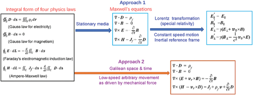
The second approach is based on the Galilean transformation, which works well for engineering applications. The moving objects or media have shapes, volumes and boundaries. The MEs-f-MDMS is to describe the electromagnetic behavior of the media that move along complex trajectory with arbitrary velocities by neglecting relativistic effects. Both approaches are for two distinctive purposes and they co-exist without any conflict with each other.

11.2. Are Maxwell’s equations covariance in moving medium?

If a point charge moves at an arbitrary speed in vacuum without the presence of any boundaries, its electric field and magnetic fields can be calculated using the Liénard-Wiechert potentials. The electric field of the moving charge contains two parts: the generalized coulomb field that does not dependent on the acceleration (also known as the velocity field), and the radiation field that is proportional to the acceleration. The free charge distribution and the instantaneous current produced by a group of moving point charges are represented by:

(79a) $\mathit{\rho }=\sum _i{q}_i\mathit{\delta }(\mathit{r}\mathit{-}{\mathit{r}}_i(\mathit{t}))$(79a)

(79b) $\mathit{J}=\sum _i{q}_i{\mathit{v}}_i(\mathit{t})\mathit{\delta }(\mathit{r}\mathit{-}{\mathit{r}}_i(\mathit{t}))$(79b)

where ${\mathit{r}}_i\left(\mathit{t}\right)$ and ${\mathit{v}}_i\left(\mathit{t}\right)$are the instantaneous position and moving velocity of the point charge $q_i$. The distribution of field in space can be calculated by substituting Equations (79a(87d) $\mathrm{\nabla }\times \mathit{H}=\mathit{J}+\mathit{\rho }\mathit{v}+\frac{\partial }{\mathit{\partial t}}\mathit{D}$(87d) -79b(79b) $\mathit{J}=\sum _i{q}_i{\mathit{v}}_i(\mathit{t})\mathit{\delta }(\mathit{r}\mathit{-}{\mathit{r}}_i(\mathit{t}))$(79b) ) into the Liénard-Wiechert potentials.

A point charge is just a point without volume and boundary. Lorentz transformation is ideal for treating the electrodynamics of moving point charges in vacuum. However, a medium is not just an aggregation of point charges, but composed of atoms with special symmetry, geometrical, shape and size. Owing to its unique crystal structure and chemistry, a medium typically has the characteristics of dielectric, electrical, magnetic and elastic properties. Therefore, it has different electrical, optical, thermal and mechanical properties. For a moving medium that has electrostatic charges on surfaces, the approach of Liénard-Wiechert potentials cannot be utilized to calculate its electromagnetic fields. This is one of the reasons why we have to expand the MEs to study the electromagnetic behavior of the motion media/object that could be time and even space dependent.

To represent the characteristics of media/materials in electromagnetic theory, the electromagnetic excitation is described by electric (P) and magnetic (M) polarizations, respectively, which was first developed over a century ago. Deepening our understanding of the electrodynamics of moving media is an important research program, which is generally through the macroscopic MEs and Minkowski material equations. In general, inhomogeneities of the velocity of a moving medium, if it is shape deformable or in liquid state, generates an inhomogeneity of the refractive index. If a medium is in a static state, the propagation of electromagnetic wave passing through it is governed by the three parameters including permittivity (ε), permeability (μ), and conductivity (σ). But each of these parameters depends heavily on the frequency of the electromagnetic wave we are considering. Electromagnetic waves with different frequencies travel at the same speed in vacuum, but they interact with media differently due to dielectric dispersion. So, variations of the permittivity, permeability and/or refractive index lead to the scattering of electromagnetic radiation of the medium.

The discussions presented above may indicate that the covariance of the MEs may not hold if there is complex media distribution in space. It would be correct to state that Maxwell’s equations perfectly fit to be Lorentz-covariant if the point charge related electromagnetic phenomena and observations are made in vacuum, otherwise the covariance may not hold.

Furthermore, we now consider the constitutive relation for a realistic medium. If one ignores the dependence of dielectric permittivity on the momentum transfer term q, for a simple linear medium, in the frequency space, we have

(80a) $\mathit{D}(\mathit{r},\mathit{\omega })=\mathit{\epsilon }(\mathit{\omega })\mathit{E}(\mathit{r},\mathit{\omega })$(80a)

In time space, and using the inverse Fourier transformation,

(80b) $\mathit{D}(\mathit{r},\mathit{t})=\underset{-\mathrm{\infty }}{\overset{\mathrm{\infty }}{\int }}\mathit{\epsilon }(\mathit{t}-t^{\mathit{\prime }})\mathit{E}(\mathit{r},t^{\mathit{\prime }})\mathit{d}{t}^{\mathit{\prime }}$(80b)

This means that if we consider the anisotropic property of a dielectric media and its frequency dependence, the constitutive relationship between the displacement vector D and electric field E cannot be simply treated as $\mathit{D}(\mathit{r},\mathit{t})=\mathit{\epsilon }\mathit{E}(\mathit{r},\mathit{t})$ unless ε is a constant. Therefore, for a general case, the covariance of the MEs holds exactly in vacuum but may not hold exactly in dielectric medium unless the medium’s property is independent of the excitation frequency ω, which means that there is no dispersion dependence. Such cases may not be true for practical materials. For an inhamogenous material, such as ferroelectric or piezoelectric crystals, the dielectric ε(ω) is described using a tensor, depending on the orientation of the medium. Therefore, the covariance of the MEs holds exactly for the electromagnetic phenomena occurring in vacuum.

11.3. About Lorentz transformation

The special relativity was proposed based on two hypotheses: I. The laws of physics take the same form in every inertial frame; II. The speed of light in vacuum is the same in every inertial frame. Special relativity is the theory of how different observers, moving at constant velocity with respect to one another, report their experience of the same physical event. General relativity addresses the same issue for observers whose relative motion is completely arbitrary. Therefore, Lorentz transformation is exact if all of the electromagnetic phenomena are in vacuum.

A key quantity in the Lorentz transformation is the speed of light c, because space and time are unified. If all of the moving point charges are in vacuum, the $c_0$ should be the speed of light in vacuum, and the situation should be easy because a point charge has no volume and boundary, and they can be represented by a set of points with charge density and related current (Equations (69(69) ${\xi }_{\alpha }{F}^{\mathit{\alpha \beta }}=\mathit{\mu }{J}^{\beta }$(69) a(25b) $\mathrm{\nabla }\cdot \mathit{B}=0$(25b) ,69b(25b) $\mathrm{\nabla }\cdot \mathit{B}=0$(25b) )). The MEs are covariant because of the use of Lorentz transformation.

However, the situation is complex if there is medium. If the entire space is filled with uniform medium so that the speed of light would be c_m = c₀/n, where n is the refraction index, the corresponding Lorentz transformation inside the medium would be [29]:

(81a) $x_m^{\prime }={\gamma }_m(\mathit{x}-v_0\mathit{t}),y_m^{\mathit{\prime }}=\mathit{y},z_m^{\mathit{\prime }}=\text{z};$(81a)

(81b) $t_m^{\mathit{\prime }}={\gamma }_m(\mathit{t}-\mathit{x}{v}_0/c_m^2)$(81b)

(81c) ${\gamma }_m=1/{(1-v_0^2/c_m^2)}^{1/2}$(81c)

Or:

(81d) $\mathit{x}={\gamma }_m(x_m\mathit{\prime }+v_0{t}_m\mathit{\prime }),\mathit{y}=y_m\mathit{\prime },\mathit{z}=z_{\mathit{m}}\mathit{\prime };$(81d)

(81e) $\mathit{t}={\gamma }_m\left(t_m^{\mathit{\prime }}+x_m^{\mathit{\prime }}{v}_0/{c_m}^2\right)$(81e)

Equations (81a–81c) hold if the medium is isotropic, and the dielectric constant and magnetic permittivity are constants, so that the speed of light in the medium is independent of the observation frame.

Now let’s consider another case, in which the space in $\mathit{x}\mathit{\prime }>0$ zone in the moving frame $\mathit{S}\mathit{\prime }$ is filled with a uniform and linear dielectric medium, and it is moving at a constant velocity $v_0$. The zone at $\mathit{x}\mathit{\prime }<0$ is vacuum. How the Lorentz transformation would be constructed to ensure the space and time continuous at the medium boundary? In practical engineering applications, part of the space is filled up with dielectric media/objects and part is vacuum, what would be the correct expression of Lorentz transformation? How do we express the unification of space and time in such a case? This question has to be investigated. Alternatively, it may indicate that the Lorentz transformation applies only to vacuum case and it may not valid if there are medium boundary in space.

To have a first try, Wang made a proposal with introduction of following expanded Lorentz transformation for the above case [5]. If we consider the dilation of time and contraction of length in relativity, an expanded Lorentz transformation for the space and time (${\mathit{r}}_m^{\mathit{\prime }},t_m^{\mathit{\prime }}$) inside the moving medium in $\mathit{x}\mathit{\prime }>0$zone could be suggested as:

(82a) $\mathit{x}={\gamma }_0(x_m^{\mathit{\prime }}+v_0{t}_m^{\mathit{\prime }}),\mathit{y}=y_m^{\mathit{\prime }},\mathit{z}=z_m^{\mathit{\prime }};$(82a)

(82b) $\mathit{t}={\gamma }_0(t_m^{\mathit{\prime }}+x_m^{\mathit{\prime }}{v}_0/c_m^2)$(82b)

Or:

(82c) $x_m\mathit{\prime }={\gamma }_m^{\mathit{2}}(\mathit{x}-v_0\mathit{t})/{\gamma }_0,y_m\mathit{\prime }=\mathit{y},z_m\mathit{\prime }=\mathit{z};$(82c)

(82d) $t_m^{\text{'}}={\gamma }_m^2(\mathit{t}-\mathit{x}{v}_0/c_m^2)/{\gamma }_0$(82d)

Here we also assume that the $\mathit{S}\mathit{\prime }$ is moving along the +x axis at speed of $v_0$. Equation (82)(87a) $\mathrm{\nabla }\cdot \mathit{D}=\mathit{\rho }$(87a) not only satisfies the continuation of the space and time at $x_m^{\mathit{\prime }}=0$ boundary, but also approaches the associated standard Lorentz transformations by replacing $c_m\to c_0$ and$c_0\to c_m$ for the cases of the entire space being vacuum and filled with a medium, respectively. One must point out that Equations (82a–82d) are just theoretical postulations, and if they are correct or not remain to be verified by experiments!

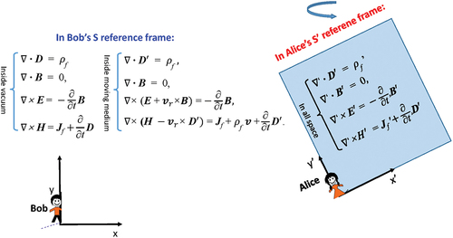
As shown in Figure 10 for a more complex case that involves accelerated motion with moving velocity much smaller than the speed of light, the field observed by Bob in the Lab frame and that by Alice may not be directly correlated by the Lorentz transformation. The equations used by Bob for describing the electromagnetic behavior are: the classical MWs equations in vacuum space; for the space inside the moving object, MEs-f-MDMS. In the reference frame in which Alice is located that moves with the moving object, since the medium is stationary for Alice, the electromagnetic behavior to be used by Alice are the MEs for the entire space. The full solutions of the equations inside and outside the medium have to satisfy the boundary conditions.

Figure 10. In the reference frame where Bob sites, there is an object/medium that is moving with acceleration and rotation. (a) The equations used by Bob for describing the electromagnetic behavior are: the classical MWs equations in vacuum space; for the space inside the moving object, MEs-f-MDMS. (b), in the reference frame in which Alice is located that moves with the moving object, since the medium is stationary for Alice, the electromagnetic behavior to be used by Alice ae the MEs for the entire space. The full solutions of the equations inside and outside the medium have to satisfy the boundary conditions.

12. Comparison with existing theories

12.1. Minkowski formulation

For a system that are made of media/objects whose shape and volumes are time-independent, if the system is moving at a constant velocity along a straight line, the field observed in the rest reference frame and that in the moving reference frame are correlated by the Minkowski formulation for ${\mathit{v}}_0\ll \mathit{c}$:

(83a) ${\mathit{E}}^{\mathit{\prime }}\approx \mathit{E}+{\mathit{v}}_0\times \mathit{B}$(83a)

(83b) ${\mathit{B}}^{\mathit{\prime }}\approx \mathit{B}-{\mathit{v}}_0\times \mathit{E}/c^2$(83b)

(83c) ${\mathit{D}}^{\mathit{\prime }}\approx \mathit{D}+{\mathit{v}}_0\times \mathit{H}/c^2$(83c)

(83d) ${\mathit{H}}^{\mathit{\prime }}\approx \mathit{H}-{\mathit{v}}_0\times \mathit{D}$(83d)

The Minskowski theory works best for medium that is not deforming, rotating or accelerating with respect to the Lab frame. In this case, both the Lab frame and moving frame are inertia frames, so that the covariance of the Maxwell’s equation preserves. However, such theory may not work well for deforming, accelerating media. In this case, the MEs-f-MDMS theory is required.

12.2. Chu formulation

The theory developed by Chu is for a case by considering a medium that may have a deformable shape and move with acceleration. His main idea is to consider an additional current source introduced by the moving medium [30]. He specifically introduced a term in the Ampere-Maxwell’s law to represent the current introduced by medium movement, the expanded Maxwell’s equtions are described by:

(84a) ${\epsilon }_0\mathrm{\nabla }\cdot \mathit{E}=\mathit{\rho }-\mathrm{\nabla }\cdot \mathit{P}$(84a)

(84b) ${\mu }_0\mathrm{\nabla }\cdot \mathit{H}=0$(84b)

(84c) $\mathrm{\nabla }\times \mathit{E}\text{ = }-{\mu }_0\frac{\partial }{\mathit{\partial t}}\mathit{H}$(84c)

(84d) $\mathrm{\nabla }\times \mathit{H}=\mathit{J}+{\mathit{J}}_p+\frac{\partial }{\mathit{\partial t}}({\epsilon }_0\mathit{E}+\mathit{P})$(84d)

where

(84e) ${\mathit{J}}_p=-\mathrm{\nabla }\times (\mathit{v}\times \mathit{P}\text{)}$(84e)

Chu treated a moving medium by considering the motion induced polarization in a medium, so that an additional current term${\mathit{J}}_{\mathit{p}}$ appears in Ampere–Maxwell law, while no change in the rest of the three equations. He derived this current term by only considering the effect of the moving boundary of the integral surface on the medium polarization term P in the integral form of the Ampere–Maxwell law [29]:

(85) ${\oint }_C\mathit{H}\cdot \mathit{d}\mathit{L}={\iint }_s\mathit{J}\cdot \mathit{d}\mathit{s}+{\epsilon }_0\frac{d}{\mathit{dt}}{\iint }_s\mathit{E}\cdot \mathit{d}\mathit{s}+\frac{d}{\mathit{dt}}{\iint }_s\mathit{P}\cdot \mathit{d}\mathit{s}$(85)

Chu’s theory is different from the MEs-f-MDMS in two points. First, Chu considered only the boundary surface movement in the mathematical derivation of $\frac{d}{\mathit{dt}}{\iint }_s\mathit{P}\cdot \mathit{d}\mathit{s}$ using the mathematical identity as given in Equation (12)(12) $\frac{\mathit{d}}{\mathit{d}t}\iint \mathit{C}\mathit{G}\cdot \mathit{\text{d}}\mathit{s}=\iint \mathit{C}[\frac{\partial }{\mathit{\partial t}}\mathit{G}+(\mathit{G}\cdot \mathrm{\nabla }\text{)}\mathit{v}+\left(\mathrm{\nabla }\cdot \mathit{G}\right)\mathit{v}-\left(\mathrm{\nabla }\cdot \mathit{v}\text{)}\mathit{G}\right]\cdot \mathit{\text{d}}\mathit{s}-\underset{C}{\oint }\left(\mathit{v}\times \mathit{G}\right)\mathit{\text{d}}\mathit{L}$(12) , but not in the calculations of $\frac{d}{\mathit{dt}}{\iint }_s\mathit{E}\cdot \mathit{d}\mathit{s}$ in Equation (85)(85) ${\oint }_C\mathit{H}\cdot \mathit{d}\mathit{L}={\iint }_s\mathit{J}\cdot \mathit{d}\mathit{s}+{\epsilon }_0\frac{d}{\mathit{dt}}{\iint }_s\mathit{E}\cdot \mathit{d}\mathit{s}+\frac{d}{\mathit{dt}}{\iint }_s\mathit{P}\cdot \mathit{d}\mathit{s}$(85) and $\frac{d}{\mathit{dt}}{\iint }_s\mathit{B}\cdot \mathit{d}\mathit{s}$ in the Faraday’s law, so that the entire mathematical calculations are not fully consistent. Therefore, in Equation (84c)(84c) $\mathrm{\nabla }\times \mathit{E}\text{ = }-{\mu }_0\frac{\partial }{\mathit{\partial t}}\mathit{H}$(84c) , the correction of the electric field on the magnetic field term ${\epsilon }_0\mathrm{\nabla }\times (\mathit{v}\times \mathit{E}\text{)}$is missed, which may miss an electromagnetic induction term owing to the medium movement to the electric field. Second, he used the magnetic field in the Lab frame $\mathit{H}$ to replace the magnetic field in the moving frame ${\mathit{H}}^{\mathit{\prime }}$, as presented in Equation (21)(21) ${\oint }_C{\mathit{H}}^{\mathit{\prime }}\cdot \mathit{d}\mathit{L}=\iint \mathit{s}\mathit{Jd}\mathit{s}+\frac{d}{\mathit{dt}}\iint \mathit{s}\mathit{D}\cdot \mathit{d}\mathit{s}$(21) , resulting in the missing of the correction term of the magnetic field on the electric field in Equation (73c)(73) $\frac{\mathit{\partial \Lambda }}{\partial A_{\beta }}-{\xi }_{\alpha }\frac{\mathit{\partial \Lambda }}{\partial ({\xi }_{\alpha }{A}_{\beta })}=0$(73) . This treatment uses the Ampere’s law for the Lab frame to replace that in the moving frame. We believe that the two points may be the major shortcomings in his theoretical approach, and the MEs-f-MDMS is more complete and comprehensive than Chu formulation for dealing the electromagnetic behavior of medium that may have a deformable shape and move with acceleration. A comparison between the Minkowski’s theory and the Chu formulation is given in [29].

12.3. Wang formulation

For easy notation, we refer the MEs-f-MDMS equations as Wang formulation [5]:

(86a) $\mathrm{\nabla }\cdot \mathit{D}=\mathit{\rho }$(86a)

(86b) $\mathrm{\nabla }\cdot \mathit{B}=0$(86b)

(86c) $\mathrm{\nabla }\times (\mathit{E}+{\mathit{v}}_r\times \mathit{B})=-\frac{\partial }{\mathit{\partial t}}\mathit{B}$(86c)

(86d) $\mathrm{\nabla }\times (\mathit{H}-{\mathit{v}}_r\times \mathit{D})=\mathit{J}+\mathit{\rho }\mathit{v}+\frac{\partial }{\mathit{\partial t}}\mathit{D}$(86d)

Now let’s assume a simple case in which the medium is moving as a solid translation $\mathit{v}(\mathit{t}$) without rotation or shape deformation, so that ${\mathit{v}}_r=0$. In this case, the Equations (86a–86d) becomes:

(87a) $\mathrm{\nabla }\cdot \mathit{D}=\mathit{\rho }$(87a)

(87b) $\mathrm{\nabla }\cdot \mathit{B}=0$(87b)

(87c) $\mathrm{\nabla }\times \mathit{E}=-\frac{\partial }{\mathit{\partial t}}\mathit{B}$(87c)

(87d) $\mathrm{\nabla }\times \mathit{H}=\mathit{J}+\mathit{\rho }\mathit{v}+\frac{\partial }{\mathit{\partial t}}\mathit{D}$(87d)

This set of equations is exactly the same as the standard MEs only with a conduction current introduced in the Ampere–Maxwell law. Therefore, the MEs hold even when the medium that moves as a solid translation even with acceleration. If the medium movement is a constant in inertia reference frame, the result from the Wang formulations is entirely consistent with that of the Minkowski’s theory under low speed approximation.

We now consider the approximated constitutive relations for the Wang formulations if the fields are expressed in two quantities. From Equation (83a–83d), and we use the constitutive relations in the rest frame for the medium, ${\mathit{D}}^{\mathit{\prime }}=\mathit{\epsilon }\mathit{E}$, and ${\mathit{B}}^{\mathit{\prime }}=\mathit{\mu }\mathit{H}$, we approximately have:

(88a) $\mathit{D}\approx \mathit{\epsilon }\mathit{E}+\mathit{\epsilon \mu }\mathit{v}\times \mathit{H}$(88a)

(88b) $\mathit{B}\approx \mathit{\mu }\mathit{H}-\text{(}\mathit{\epsilon \mu }-{\epsilon }_0{\mu }_0\text{)}\mathit{v}\times \mathit{E}$(88b)

Note, the term $\text{(}\mathit{\epsilon \mu }-{\epsilon }_0{\mu }_0\text{)}$ is a result of using the Lorentz transformation in vacuum for medium case. We are not sure if this make sense in physics or not, but do appear in literature as a result of mathematical calculation [17].

13. Contributions made by the MEs-f-MDMS

This paper systematically reviews the recent progress made in developing the Maxwell’s equations for a mechano-driven media system (MEs-f-MDMS), which are utilized to describe the electromagnetism of multi-moving-media. The fundamental theoretical advances are summarized as:

1. Based on the integral forms of the four physics laws, and in the Galilean space-time, the MEs-f-MDMS are derived to describe the electrodynamics of slow-moving media that may move with acceleration.

2. The MEs-f-MDMS are typically used to reveal the dynamics of an electromagnetic field for a general case, in which the medium has a time-dependent volume, shape, and boundary and may move in an arbitrary velocity field ${\mathit{v}}_r$(r, t) in a non-inertial system.

3. By neglecting the relativity effect, the MEs-f-MDMS are applicable to reveal the electrodynamics of a mechanical force-electricity-magnetism system.

4. The total energy of electricity and magnetism is not conserved, since an external mechanical energy is input; however, the total energy of the closed mechano-driven media system is conserved.

5. The charged moving media are regarded as the sources distributed inside the media for generating electromagnetic radiation in space (a motion-generated electromagnetic field). The created electromagnetic wave within the moving media can be described by the expanded MEs-f-MDMS, and its propagation in space satisfies the standard MEs and special relativity; they meet at the medium interface as governed by the boundary conditions.

6. Different from the methods of relativity electrodynamics that the electromagnetic fields in the Lab frame and the co-moving frame are correlated by the Lorentz transformation provided the MEs are covariant. The expanded MEs-f-MDMS are for the case that the observe is in the Lab frame, while the media are moving at complex velocities along varies trajectories. In other words, all fields are expressed in the variables in the Lab frame, which is more useful for describing engineering problems.

7. Because the speed of light inside media c_m is generally lower than c₀, there is no need to worry about exceeding the speed of light in vacuum c₀ even the medium is moving. Once the electromagnetic wave is generated from the mechano-driven media system, its traveling outside the medium is governed by the classical MEs, regardless of whether the media are moving or not.

8. The expanded MEs-f-MDMS could describe the electrodynamics of fluid/liquid media, because it has been proved that these equations can describe the electromagnetism of the mechano-driven system in the non-inertial frame with acceleration and even time-dependent volume, shape, and boundary.

9. If the medium moves at a constant velocity so that $\mathit{v}$ = constant and ${\mathit{v}}_r$ = 0, MEs-f-MDMS resume the format of the classical MEs, so there is no logic inconsistency with the existing theory.

10. The MEs were derived by assuming that the objects/medium are at stationary with respect to the observer. The covariance of the MEs is thus preserved under Lorentz transformation. However, since MEs-f-MDMS were derived by assuming that the objects have accelerated motion with respect to the observer, they thus may not be covariant under Lorentz transformation. Therefore, Lorentz transformation is applicable if there are no medium boundaries in space. How to expand the Lorentz transformation to cases there are medium boundaries remain to be further studied, although we have made a first proposal (see Equation (82)(87a) $\mathrm{\nabla }\cdot \mathit{D}=\mathit{\rho }$(87a) ).

In comparison to the classical MEs, the MEs-f-MDMS has made following contributions:

1. Accelerated motion in a non-inertia reference frame vs that with a uniform motion along a straight-line in inertia reference frame;

2. Electromagnetism that includes the Feynman ‘anti-flux rule’ examples vs that exclude such cases;

3. Electrodynamics for multi-moving-media vs that for one moving medium; and

4. The entire field (both near field and far-field) electrodynamics vs the far-field plus partial near-field electrodynamics.

Much of the traditional research is focusing on the far-distance transmission and reflection of electromagnetic waves, for instance wireless communication & propagation, antenna, radar, and so on, demonstrating through the special solutions of the MEs. The effects from the motion status of the electric current source and the mechanical action for generating the current to the distribution of electromagnetic fields in the vicinity have been ignored. Such near-field effect can be important for new technological applications in short-range wireless sensing. MEs-f-MDMS provide an accurate and practical method to systematically investigate both the far-field electromagnetic behavior and the near-field electromagnetic behavior for engineering applications.

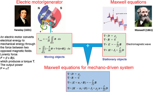
MEs-f-MDMS is a unification of the theory for electromagnetic generator/motor and the theory of electromagnetic waves (Figure 11). The theory of electromagnetic generator is to use the rotation of a rotor to cut through a magnetic field, so that the mechanical energy is converted into electric power. What is most important is the electric current and voltage carried by the conduction coil, disregard the electromagnetic wave radiated to the space nearby. The MEs are about the electromagnetic waves radiated if an oscillating current is supplied. Once the observation point is close to the electromagnetic generator, near to which the rotation of the rotor is quite dominant, the MEs can predict the electromagnetic behavior arising from the current conducted in the metal wire, but it may not precisely predict the effect of the rotating rotor to the field distributed nearby. This is why we need the MEs-f-MDMS.

Figure 11. The MEs-f-MDMS are a unification of the theory for electromagnetic generator/motor and the theory of electromagnetic waves, so that the field in the entire space can be calculated. MEs-f-MDMS are likely to make a key difference in the regions near the moving objects, which may not be fully covered by the classical MEs. This is the contribution of the MEs-f-MDMS to the fundamentals of electrodynamics.

14. Potential applications

Previously, the MEs can be effectively calculate the electromagnetic behavior of stationary media, which covers most of the scenarios in physics and engineering applications. The electromagnetic radiation produced by an accelerated moving object can by calculated using the MEs-f-MDMS, such as the electromagnetic radiation distributed around a power generator or a wind mill. In this case, the rotation of the medium is likely to introduce additional component in the near-field field. The movement of the object is like to be a source for generating electromagnetic wave, and the propagation of the waves in the space is governed by the classical Maxwell’s equations.

Traditionally, electromagnetic waves are usually generated by oscillating current through an open antena. An important application of MEs-f-MDMS is to generate low-frequency electromagnetic wave using the relative rotation of media, such as rotation mode TENG, so that the radiated wave can reach a far distance in medium such water. In such a case, one can generate low-frequency signal by a confined device that is much smaller than the size of traditional antenna. This could find application for communications underwater.

In today’s technology, the moving velocity of an object can be multiple times of the speed of sound. In such a case, the movement of the object can be seriously affect the phase of the electromagnetic waves. For a jet that is flying at a speed of 3 km/s and is located at a distance of 100 km, the electromagnetic wave will take 0.3 ms to reach the aircraft surface. With considering the time required from signal processing the recording, the elapsed time is in the order of 1–5 ms, during which the aircraft would fly for a distance of 3–15 m, which could be longer than the length of the jet. In this case, if we donot consider the movement of the jet in the theoretical modeling, the calculation result can be far from the realistic case for traditional Radar to capture the position of the flying jet. If one uses the phase information for Radar detection, such a distance would create a gigantic phase shift if the communication is in the order of GHz. We anticipate that MEs-f-MDMS would find more applications in engineering.

Acknowledgments

Thank to Drs. Jiajia Shao and Wei Tang for many stimulating discussions.

Disclosure statement

No potential conflict of interest was reported by the author.

References

- Minkowski H. The principle of relativity. Calcutta: University Press; 1920.
- Minkowski H. Das Relativitätsprinzip. Ann Phys. 1915;352:927–938. doi: 10.1002/andp.19153521505
- Pauli W. Theory of relativity. London: Pergamon; 1958.
- Landau LD, Lifshitz EM, Pitaevskii LP. Electrodynamics of continuous media. (NY): Pergamon Press; 1984.
- Wang ZL, Shao J. Recent progress on the Maxwell’s equations for describing a mechano-driven medium system with multiple moving objects/media. Electromag Sci. 2023;1:1–16. arXiv preprint arXiv:2306.02535. doi: 10.23919/emsci.2023.0017
- Born M. Einstein’s theory of relativity. (NY): Dover Publications; 1962.
- Le Bellac M, Lévy-Leblond JM. Галилеевский электр омагнетизм. Nuovo Cim B. 1973;14:217–234. doi: 10.1007/BF02895715
- Rousseaux G. Forty years of galilean electromagnetism (1973–2013). Eur Phys J Plus. 2013;128:1–14. doi: 10.1140/epjp/i2013-13081-5
- Zangwill A. Modern electrodynamics. UK: Cambridge University Press. Section 22.6.3. 2012.
- Levy-Leblond JM. Une nouvelle limite non-relativiste du groupe de Poincare. Ann Inst Henri Poncare, Section A Physique Theorique III. 1965;3:1–12. http://www.numdam.org/item/AIHPA_1965__3_1_1_0/
- Feynman RP. The Feynman lectures on physics, vol. II: mainly electromagnetism and matter. New Millennium Ed. New York: Basic Books; 2011.
- Crooks MJ, Litvin DB, Matthews PW, et al. One-piece Faraday generator: a paradoxical experiment from 1851. Am J Phys. 1978;46:729–731. doi: 10.1119/1.11109
- Guala-Valverde J, Mazzoni P, Achilles R. The homopolar motor: a true relativistic engine. Am J Phys. 2002;70:1052–1055. doi: 10.1119/1.1498857
- Wang ZL. The expanded Maxwell’s equations for a mechano-driven media system that moves with acceleration. Int J Mod Phys B. 2022;37:2350159. doi: 10.1142/S021797922350159X
- Wang ZL. On the expanded Maxwell’s equations for moving charged media system-general theory, mathematical solutions and applications in TENG. Mater Today. 2022;52:348–363. doi: 10.1016/j.mattod.2021.10.027
- Wang ZL. Maxwell’s equations for a mechano-driven, shape-deformable, charged-media system, slowly moving at an arbitrary velocity field v(r,t). J Phys Commun. 2022;6:085013. doi: 10.1088/2399-6528/ac871e
- Rozov A. Maxwell equations for slow-moving media. Z Naturforsch. 2015;70:1019–1024. doi: 10.1515/zna-2015-0142
- Scanlon PJ, Henriksen RN, Allen JR. Approaches to electromagnetic induction. Am J Phys. 1969;37:698–708. doi: 10.1119/1.1975777
- Zhao K. Examples for disapprove flux rule. University Physics. Beijing: High Education Press; 1985. p. 10–13.
- Zangwill A. Modern electrodynamics. UK: Cambridge Press. Section 14.4.1. 2012.
- Jackson JD. Classical electrodynamics. 3rd ed. New York: John Wiley & Sons; 1999.
- Thakkar V, Niser IM, Mohapatra A. Faraday’s law in moving media; 2015. Available from: https://www.researchgate.net/publication/29946116
- Becker R. Electromagnetic fields and interactions. New York: Dover Publications; 1964.
- Wang ZL. On the first principle theory of nanogenerators from Maxwell’s equations. Nano Energy. 2020;68:104272. doi: 10.1016/j.nanoen.2019.104272
- Wang ZL. From contact electrification to triboelectric nanogenerators. Rep Prog Phys. 2021;84:096502. doi: 10.1088/1361-6633/ac0a50
- Lax M, Nelson DF. Maxwell equations in material form. Phys Rev B. 1976;13:1777–1784. doi: 10.1103/PhysRevB.13.1777
- Crater HW. General covariance, Lorentz covariance, the Lorentz force, and the Maxwell equations. Am J Phys. 1994;62:923–931. doi: 10.1119/1.17682
- Available from: https://en.wikipedia.org/wiki/Covariant_formulation_of_classical_electromagnetism
- Penfield P, Hermann AH. Electrodynamics of moving media. Cambridge (MA): The MIT Press; 1967.
- Fano RM, Chu LC, Adler RB. Electromagnetic fields, energy and forces. New Yo(NY): John Wiley & Sons, Inc; 1960.