Geomorphology, Land-Use, and Hemeroby of Foothills in Colombian Orinoquia: Classification and Correlation at a Regional Scale

Abstract

In the management of ecosystem services, it is significant to relate land use with the physical characteristics of the terrain, which allows establishing the conditioning factors of human activities and planning their distribution. These analyzes are based on thematic cartography, usually generated with visual classifications of satellite images. Traditional mapping techniques involve limiting the timely availability of information by taking extended periods for interpretation and integration of multiple data sets. This article presents a methodology to overcome these difficulties, implements machine learning and cloud computing to generate timely thematic cartography and spatial analysis to support land use planning. The study area was delimited according to altitudinal levels that define braided and anastomosed river systems. Acquisition, processing, and classification of input data for modeling were performed on the Google Earth Engine platform. The spatial correlation between hemeroby and geomorphology was calculated with the odds ratio and its respective confidence interval. Maps of 27 geomorphological units, 11 types of land use, and six hemeroby levels are presented at a scale of 1:50,000. Confusion matrices of implemented classification models were also reported, allowed evaluating global, user’s, and producer’s accuracy. Correlations between relict of natural areas with the structural environment and urban infrastructure with alluvial fans stand out. The information generated by these procedures is essential for planning land use and prioritizing the maintenance of ecosystem services.

Keywords:

• Geomorphology
• land-use
• hemeroby
• Orinoquia
• remote sensing
• Google Earth Engine
• Random Forest

Introduction

The Colombian Orinoquía has been influenced by climatic, tectonic, and depositional events (Jaramillo and Rangel-Ch 2014a, 2014b). These conditions have generated real and potential instability in the foothills, where sediment transport from the Andean cordillera to the alluvial plain can become torrential (IDEAM 2010a). The foothills are a limitedly available area for receiving materials transported by fluvial-torrential events; they are mainly constituted by debris flows associated with chaotic sedimentation processes, which configure scenarios of geomorphological threat for the populations settled in the territory (Méndez et al. 2016). Mass removal events, sudden floods or torrential avalanches are related to the acceleration of morphodynamic processes such as erosion, riverbed changes and sedimentation, caused by the change in natural covers to establish agricultural activities (Robertson and Castiblanco 2011). The development of the towns in the Orinoquia is related to the proximity to the main rivers and the roads that go to the interior of the country. The main towns of the Orinoquia, foothills have the highest population densities in the region and provide social infrastructure and services, giving the inhabitants elements for the articulation of the main productive activities, based on the collection and marketing of agricultural goods (IGAC 2004). Given these characteristics, planning land use in the foothills requires cartographic inputs and spatial analysis that establish the environmental conditioning factors of land appropriation.

Environmental and socioeconomic decision-making has often been based on thematic mapping in the last few decades (Foody 2004; Jin, Stehman, and Mountrakis 2014; Powell et al. 2004). Mapping the distribution and dynamics of land use is essential to understand terrestrial processes, including biogeochemical cycles and biodiversity (Giri et al. 2013). In addition, for the management of ecosystem services, the differentiation and quantification of land use can help explain the relationship between man and the environment (Tsai et al. 2018; Vega et al. 2018; Xie, Sha, and Yu 2008). Remote sensing-based mapping is the fastest and most efficient way to quantify and monitor landscape structure (Steinhardt et al. 1999), both for geomorphological aspects (Silva and Alves 2007; Almeida and Luchiari 2017) and land use (Salovaara et al. 2005; Tsai et al. 2018; Vega et al. 2018). However, mapping based on satellite images presents challenges such as landscape complexity, the choice of input data, the definition of processing and classification techniques, and ambiguous spectral responses (Thenkabail et al. 2003; Domaç and Süzen 2006; Lu and Weng 2007; Xie, Sha, and Yu 2008).

Colombia adapted the CORINE (Coordination of Information on the Environmental) Land Cover methodology to generate its official land use cartography. It is a European visual classification technique at a 1:100,000 scale, based primarily on medium resolution optical images (IDEAM 2010b). Classification of optical images is based on reflectivity of differential coverages (Azzari and Lobell 2017; Stone et al. 1994). Moreover, in Colombia, there is a systematic methodological proposal for analytical geomorphological mapping (SGC 2015). But these maps are not yet available on a regional scale for the study area and are usually made according to visual interpretations of aerial photographs. Digital analysis of patterns derived from remote sensors for the classification of geoforms represents a principal field of study (Franklin and Peddle 1987; Paradella et al. 2005). These methodological applications are based on the location and distribution of the landforms, terrain elevation, surface composition, and subsurface characterization (Smith and Pain 2009).

At present, Synthetic Aperture Radar (SAR) images have made great advantages by providing information on the physical and dielectric properties of the terrain, under all weather conditions and during day or night (Du et al. 2015; Flores-Anderson et al. 2019; Moreira et al. 2013; Paradella et al. 2005; Topouzelis and Psyllos 2012). Recent technological advances in these systems include high spatial resolution and an increase in the repetition rate in obtaining data in a dependable, continuous, and global way (Moreira et al. 2013; Du et al. 2015; Flores-Anderson et al. 2019). According to the frequency of the signal, SARs have different penetration capabilities (Meyer 2019; Walsh, Butler, and Malanson 1998). In the context of this research, L-band SARs, because they are low frequencies, allow obtaining information on the texture and humidity of the terrain. While the C-band SARs provide information about the physiognomic structure of the covers, the Digital Elevation Models (DEM) obtained from SAR image interferometry allow the calculation of parameters such as slope and aspect of the terrain (Bocco, Mendoza, and Velázquez 2001; Grohmann, Riccomini, and Steiner 2008; Silva and Alves 2007; Smith and Pain 2009).

In addition to the wide availability of optical and SAR images, their integration is a frequent practice today, although not yet implemented in the available cartography of the study area. These multi-sensor inputs allow highlight geomorphological, geobotanical, and anthropic characteristics of the landscape (Castañeda and Ducrot 2009; Grohmann, Riccomini, and Steiner 2008; Hamilton et al. 2007; Paradella, Bignelli, and Veneziani 1997; Reiche et al. 2016; Souza and Paradella 2002). Quantitative information derived from remote sensing and DEMs is also frequently used as inputs to classification models (Walsh, Butler, and Malanson 1998; Smith and Pain 2009; Colditz 2015). The Normalized Difference Vegetation Index (NDVI), calculated from optical images, is of interest in the context of the study. Terrain characteristics originated from a DEM, such as slope, aspect, roughness, and convexity, are also relevant.

There is a large amount of global satellite information collected over decades, limiting traditional mapping techniques implemented at regional scales. These restrictions are represented by the computational and storage capacity to analyze the available data. Cloud computing can overcome these technical barriers and constitutes a resource for the timely availability of information to support land use management (Azzari and Lobell 2017; Perilla and Mas 2020). Google Earth Engine (GEE) is an automated parallel computing platform that publicly stores petabytes of remote sensing information on a planetary scale (Kumar and Mutanga 2018; Mutanga and Kumar 2019). GEE outpaces local processing of images downloaded from external repositories employing traditional techniques, and integrates a varied of functions that can be used with great versatility through programming languages such as Python or JavaScript (Reiche et al. 2016; Gorelick et al. 2017).

Visual interpretation supports the geomorphological and land use mapping available for the study area; however, there is established enhanced digital analysis available including the implementation of machine learning to delineate landscape conditions. During the last decades, those based on Machine Learning have received particular attention for obtaining highly accurate results. These techniques rapidly process and non-parametric, facilitating the classification of remote sensing data that do not follow a normal distribution (Akar and Güngör 2012; Shetty 2019) and multidimensional images with numerous stacked bands from various sources (Waske and Braun 2009). Random Forest is an outstanding technique that implements multiple user-defined decision trees in random subsets with sample replacement (bagging). Samples in training areas can be selected more than once for training and have high variance with low bias. The mean of the probabilities assigned to all the trees defines the final ranking, making the model less sensitive to extreme values and overfitting (Pal 2005; Akar and Güngör 2012; Belgiu and Dragut 2016).

Environmental indices are essential in land use management, but they have little representation in the study area. These indices provide information on the state of ecological systems, support decision-making, and uphold the monitoring and evaluation of political and administrative efforts on land use (Steinhardt et al. 1999). Not yet implemented in the Colombian Orinoquia, the hemeroby index is a comprehensive estimator of human impact on natural systems, considering the relationship between current land use and vegetation that would exist in the absence of anthropic disturbances (Steinhardt et al. 1999; Peterseil et al. 2004; Walz and Stein 2009). This indicator shows inequities between conservation areas and land use planning, points out areas that require measures to improve the environmental conditions of the landscape, and highlights the advances in environmental management (Walz and Stein 2009). These inequities indicate the differential use of ecosystem services in densely populated areas, whose demand is proportional to the established human population and where natural areas are transformed to maximize certain benefits to the detriment of others (Schneiders and Müller 2017).

Cartographic problems in the foothills in Colombian Orinoquia constitute a barrier to the management of land use. This article considers methodological tools that allow overcoming: the insufficiency of maps that articulate different complementary satellite sources; the absence of classification techniques without the subjectivity of visual interpretation; and the lack of indices that establishing the degree of human intervention according to the terrain. In order to generate timely thematic cartography and comprehensive analysis of the landscape, this research proposed: (1) mapping geomorphology and land use of foothills in Orinoquia through multi-sensor images and classifications with Machine Learning methodologies on the GEE platform; (2) mapping hemeroby or levels of human intervention in the landscape, according to cartographic integration of land use, roads, oil wells, and mining concessions; (3) estimate the quantitative correlation of geomorphological units and hemeroby levels.

Materials and methods

Study area

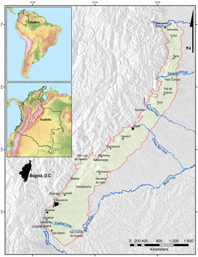
Goosen (1963, 1964) associated the landscapes of the Orinoquia with physiographic units and defined the foothills as the area encompassing the ancient alluvial fans of the early and middle Pleistocene. These can be folded, raised near the mountain ranges, or covered by recent sediments. The study area covers 18,817 km², delimited to the North by the Arauca River and to the South by the Ariari River basin. Altitudes defined by Jaramillo and Rangel-Ch (2014b) delimited East and West sides; they established that the braided and anastomosed river systems, characteristic of the foothills, settle in areas of intense slope discontinuities between Cordillera, the foothills, and the floodplain. These ruptures occur at higher altitudes in the South due to the flexing of crust in the Altillanura.

To exclude the Andean region of the Eastern Cordillera to Westside, and Altillanura and Floodplain to East, different altitude levels according to basins located in foothills were drawn: South of Meta River, in Guamal River Basin, 575 m as an upper level and 350 m as a lower level; toward North of Meta River, 675 m and 200 m levels for Meta and Pauto River basins, 600 m and 200 m for Casanare River Basin, 425 m and 200 m for Cravo Sur River and 375 m and 175 m for Arauca River (Figure 1). The vector layer of the hydrographic zoning of Colombia to define the river basins of the foothills was employed (IDEAM 2013). The 30 m DEM data generated from NASA’s Shuttle Radar Topography Mission (SRTM v.3, available at GEE) was used to establish the altitude (Farr et al. 2007).

Figure 1. Study area.

Methodological structure

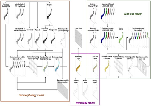
Presented modeling implements integrated systems, in which the outputs or results of some models define the inputs or parameters of subsequent models. Figure 2 shows the integration of the models, which correspond to geomorphological, land use, and hemeroby levels. The input data for the geomorphological model included DEM and L band SAR images, while the inputs for the land-use model corresponded to optical and C band SAR images. In the hemeroby model, the output of the land-use model was included as input, together with secondary cartographic information of oil wells, roads, and mining concessions. Correlation between levels of human intervention and geoforms was calculated according to the count of hemeroby pixels included in each geomorphological class.

Figure 2. Methodological synopsis.

Input data

Input data from remote sensors were collected in raster format with a spatial resolution of 30 m, data with a higher resolution was rescaled so that its pixel size matched. Satellite images were filtered in the GEE according to the period of interest and the study area. Additionally, SAR images were filtered based on specific polarizations, modes, and orbits. The geomorphological model included two L-band SAR polarizations and five parameters considered as fundamental descriptors proposed by (Franklin 1987; Franklin and Peddle 1987): (1) HH/HV polarizations of a 2018 Alos-PalSAR yearly mosaic (Global PALSAR-2/PALSAR collection, available from GEE), with a Speckle correction (Raed et al. 1996) performed by a 50 m focal mean filter to increase the accuracy of image classification (Waske and Braun 2009); (2) DEM NASA SRTM v.3, from which they derived slope, aspect, and convexity layers; (3) slope or inclination of the terrain in percentage, classified in ordinal categories according to the typology of slope classes proposed by Instituto Geográfico Agustín Codazzi (IGAC 2014); (4) aspect or orientation of slope in degrees concerning North; (5) convexity calculated from the relative elevation of a seven-pixel moving window concerning its surroundings, in terms of concave (relative altitude of moving window less than vicinity), convex (higher relative altitude), and flat (similar relative elevation); (6) roughness or irregularity of terrain, calculated with an analysis of local variance of the slope (seven pixel moving windows).

Land use model included as input data: (1) Sentinel-1 image mosaics (S1 GRD collection, available at GEE) obtained during 2019, of VV/VH polarizations in interferometric wide fringe mode, descending orbit, and with a focal mean filter at 50 m for Speckle correction; (2) Landsat-8 images (T1 SR collection, available at GEE) obtained during 2019, visible spectrum (RGB), near-infrared (NIR), and short wave infrared (SWIR) bands, were included. A QA-band-based function masked Landsat collection to later calculate a mosaic with the mean of the pixel values, function CFMask (C code based on the Function of Mask) is a multi-pass algorithm that uses decision trees to select clouds and shadows to define a binary image with argument “0” where the chosen pixels coincide (Foga et al. 2017); (3) NDVI calculated and added to the model, based on bands in the red and near-infrared spectrum, which partially suppresses the influence of lighting, terrain heterogeneity, and ground reflectance on image data (Tsai et al. 2018).

Training areas

The performance of supervised classification of satellite images not only depends on the robustness of the classifier, but the quality of the training samples is also relevant, which unequivocally represents thematic categories in the multidimensional image (Olofsson et al. 2014). Assignment of training areas considered the spectral amplitude of images and the landscape representativeness of classes since balanced samples between thematic categories present greater accuracy by reducing the commission and omission error of under-represented classes (Jin, Stehman, and Mountrakis 2014; Tsai et al. 2018). Pixels included in training areas were divided into 70 percent for predictions and the remaining 30 percent to calculate the accuracy of the classifications (Azzari and Lobell 2017), which guaranteed the statistical independence of the validation data and limited the overestimation of the model’s accuracy (Congalton 1991; Belgiu and Dragut 2016).

Geomorphological model training areas were established with digital altitude profiles based on DEM and visual interpretation of L band SAR images. Eighty-nine polygonal entities of 27 geoforms were delineated, identified according to the geomorphological units described by the Servicio Geológico Colombiano (SGC 2015). Geomorphological training areas covered 28.16 percent of foothills, ensuring the representativeness of the sample, which is valid in proportions greater than 0.25 percent of the study area (Colditz 2015).

Training areas of the land use model were defined based on the spatial entities of the map of terrestrial ecosystems of Colombia (IDEAM 2017). One hundred six polygons belonging to 11 land use classes of this cartography were selected and spatially refined through visual reinterpretations based on pictorial and morphological characteristics of the input data. Land use training areas covered 24.43 percent of foothills, which validated the representativeness of the sample. Although agricultural areas present typical spatial patterns, temporal dynamics and interaction with electromagnetic spectrum captured by sensors are not constant due to the different phenological stages of crops (Waske and Braun 2009). These limitations cause cultivated areas to be confused with introduced pastures dedicated to livestock, for such reason both units merged in the same category called agricultural.

Setting parameters of Random Forest

Theoretically, it is assumed that the greater the number of trees, the better fit of the Random Forest models; although the processing time increases linearly concerning this parameter, justifying the adjustment of the classifier with an optimal number of trees (Probst, Wright, and Boulesteix 2019). Sampling variables defined with multidimensional images and vector layers of training areas configured the Random Forest; vector fields, with thematic categories in a numerical format, were also specified. Next, samples were divided into 70 percent for training and 30 percent to estimate accuracy, through an iterative function, in a sequence of every five trees, until completing 100 trees. Finally, predictions were made according to the sampling variable and the sequential parameters of trees, allowing plotted accuracy according to the number of trees in the Random Forest classification.

Random Forest classification and estimation of error

In this step, input layers and sampling areas defined training variables for Random Forest classifiers in each case, similar to sampling variables implemented during parameterization procedures. Next, training variables and the number of trees that obtained the highest accuracy configured the classifiers. Classification results were exported in raster format, at a spatial scale like that of the input layers. Subsequently, classifications were converted to vector format, with a minimum mappable area of 10 ha.

Same training variables from Random Forest models and the number of previously defined classification trees were used as parameters to calculate the accuracies (Pal 2005). The training areas were divided similarly to the parameterization procedures (70 percent − 30 percent). Accuracy estimates included confusion matrices, the overall accuracy of models, the producer/user accuracies, and Kappa coefficients. The confusion matrix is a square array, where the number of pixels is correctly classified between the sample, they arrange on the diagonal (Liu, Frazier, and Kumar 2007). This matrix allows evaluating the general accuracy of classification, calculated as the quotient between the number of correctly classified pixels and the total number of pixels in the sample (Plourde and Congalton 2003). The user’s accuracy estimates the proportion of pixels in each category classified according to training, while the producer’s accuracy calculates the fraction of correctly classified reference pixels (Story and Congalton 1986; Congalton 1991). The producer’s accuracy allows us to establish by complementarity the error of omission or proportion of pixels not included in the same class of the training area; whiles the user’s accuracy does the same with the commission error, which establishes the proportion of pixels erroneously assigned to a class during training (Stehman 1992). The Kappa coefficient is an estimate of the difference between accuracy achieved by a parameterized classifier versus a classification performed randomly (Rosenfield and Fitzpatrick-Lins 1986; Plourde and Congalton 2003).

Hemeroby and its correlation with Geomorphology

To obtain the spatial distribution of hemeroby levels was integrated by overlaying to the land-use layer, the geographic information corresponding to: (1) roads represented by line-type vectors available in the basic cartography of the Colombian territory (IGAC 2017), buffers were drawn at a distance of 0.5 km around paved roads with two or more lanes, 0.2 km around unpaved roads with two or more lanes, and 0.1 km around narrow paved roads; (2) oil wells represented by point features available in the Banco de Información Petrolera (SGC 2019), buffers were plotted 1.0 km away; (3) mining concessions represented by polygons available in the Catastro Minero Colombiano (ANM 2019). Nominal classes obtained in the cartographic integration were reclassified into ordinal categories, according to the compilation and assignment of hemeroby levels to land uses proposed by Steinhardt et al. (1999) and Walz and Stein (2009).

The Odds Ratio (OR) compares independent binomial proportions in double-entry contingency tables and allows measuring the direction and magnitude of the discrepancy between the values (Lawson 2007). To calculate the OR between the values under consideration, each proportion is transformed into Odds, defined as the ratio between the probability that the event occurs and the probability that it does not. The comparison between Odds is done using its own ratio, consequently called Odds Ratio, where the focal ratio is compared to the reference ratio (Rita and Komonen 2008). Correlation between geomorphology and hemeroby was calculated with the odds ratio (OR) and 95 percent confidence intervals (CI95%). OR calculation considered the overlap between the pixel count at 30 m of the hemeroby levels in the identified geomorphological areas. Statistically significant correlations were considered those with a p-value less than 0.05 and with an interval confidence of 95% excluding the value of one.

Results and discussion

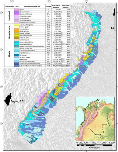
Figure 3 shows the geomorphological map. The geoforms of the fluvial environment predominate with 81 percent of the foothills, in particular sub-recent accumulation terraces, current alluvial fans, and ancient accumulation terraces. The term sub-recent describes an intermediate relative age if it is possible to differentiate two or more adjacent fans (SGC 2015). The denudational environment covers 12 percent of foothills, where erosive and undulating hillsides prevail. With the smallest extension, the structural environment occupies 7 percent of the study area, with a predominance of hills and ridges of a structural nature.

Figure 3. Geomorphological map.

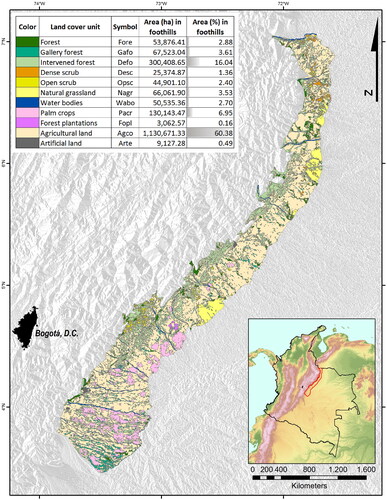
On the land use map (Figure 4), areas dedicated to agricultural production predominate. The distribution of land use has been influenced by the expansion of livestock and monocultures such as African palm and rice (Romero-Ruiz et al. 2011). Among forest covers, degraded forests have the highest proportion of area, while natural grasslands predominate in low coverages. According to the proportion of areas intervened by anthropic activities, it is evident that humans have transformed 87.28 percent of the original covers of foothills, and steep terrain still maintains relics of natural forests, whose slope and edaphic characteristics do not facilitate contemporary agricultural activities. Although continued logging has changed the forest structure across rugged terrain in many locations, agriculture has not been a transformational agent in these areas. Originally forested areas in more advanced stages of degradation are currently covered by shrubbery. Shrub vegetation is often located on the flat terrain of the fluvial environment, where selective logging becomes widespread to establish agricultural activities (Niño et al. 2019). This distribution of coverages is the result of government initiatives that postulate the Orinoquia as one of the regions with the greatest agro-industrial and extractive potential in the country (PNN 2014). Anthropic processes such as the expansion of the agricultural frontier have drastically modified biophysical conditions of the landscape during the last six decades, which puts the permanence of ecological systems at risk (Rangel-Ch and Minorta-Cely 2014).

Figure 4. Land-use map.

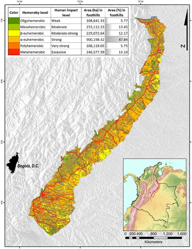
Map of levels of hemeroby (Figure 5) presents in detail the diversity of human impact on foothills. According to the spatial representativeness of areas classified in hemeroby levels, it is observed that (1) α-euhemerobic level predominates in the study area, characterized by intensive agricultural and livestock activities; (2) it is followed to a lesser extent by areas with a mesohemerobic level, where intervened forests that have lost their original structure prevail; (3) followed by zones with a metahemerobic level, occupied by urban infrastructures and areas influenced by roads; (4) continuing areas with a β-euhemerobic level, used for forest plantations and oil palm or covered by scrub on originally forested areas; (5) followed by zones of oligohemerobic level, where blocks of isolated forests subject to selective thinning predominate; (6) and finally, areas with a polyhemerobic level, dedicated to the extraction of minerals and oil. There is no evidence of areas exempt from human intervention in foothills; therefore, the ahemerobic level was not representative in the studied area.

Figure 5. Hemeroby map.

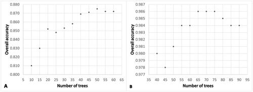
Parametrization of the geomorphological classifier with 50 decision trees obtained the highest model accuracy, calculated at 0.875. That is, 87.5 percent of pixels classified in training areas coincided with categories defined in the sample (Figure 6A). Regarding the land use classifier, 65 decision trees obtained the highest accuracy, with which 98.6 percent of pixels were classified correctly, according to training areas (Figure 6B).

Figure 6. Parametrization of the classifiers Random Forest. (A) For geomorphological model; (B) for land-use model.

Table 1 contains the confusion matrix calculated for the geomorphological model. The higher omission error occurred in incised alluvial fans, where 27.8 percent of pixels they classified within other geomorphological units, mainly as accumulation terraces or current alluvial fans. Floodplains follow with 18.9 percent omission, mostly misclassified as sub-recent accumulation terraces or actual alluvial fans. Ancient undifferentiated alluvial fans presented higher commission error, with 34.0 percent of pixels classified as different units, mainly as actual alluvial fans or floodplains. Dejection cones follow with 32.1 percent commission, mostly misclassified as actual alluvial fans or incised alluvial fans. Calculation of the Kappa coefficient made it possible to establish the probability of making a correct classification at 0.86, compared to a classifier that randomly assigns pixels to different geomorphological classes.

Table 1. Confusion matrix of the geomorphological model.

CLASS^a	Fcaf	Faaf	Fauaf	Fiaf	Fsaf	Fdc	Ffs	Fts	Ssi	Dag	Deg	Dehs	Shs	Duhs	Ddh	Sh	Sol	Ddl	Sl	Drl	Dftl	Scap	Ffp	Ss	Fat	Faat	Fsat	User’s
Fcaf	2,321	54	116	45	13	52	20	1	0	0	0	2	0	1	3	4	0	1	0	0	9	2	37	0	34	19	23	0.842
Faaf	68	2,278	3	5	150	3	2	1	0	19	3	7	2	15	2	5	0	0	0	0	27	6	0	0	6	22	0	0.868
Fauaf	1	0	719	4	0	2	2	0	0	0	0	0	0	0	2	0	0	0	0	0	1	0	4	0	3	0	4	0.969
Fiaf	228	217	68	3,801	145	25	20	3	0	0	3	0	0	12	12	2	0	0	2	3	37	13	52	3	382	227	9	0.722
Fsaf	2	3	1	0	816	1	1	1	0	1	2	7	0	6	1	0	0	1	0	1	8	2	0	0	3	13	0	0.938
Fdc	0	0	0	0	0	201	0	0	0	0	0	0	0	0	0	0	0	0	0	0	0	0	0	0	0	0	0	1.000
Ffs	1	0	4	7	0	0	345	0	0	0	0	0	0	1	2	0	0	2	0	0	1	0	3	0	2	1	0	0.935
Fts	0	0	0	0	0	0	0	119	0	0	0	0	0	1	0	0	0	0	0	0	0	0	0	0	0	0	0	0.992
Ssi	0	0	0	0	0	0	0	0	34	0	0	0	0	0	0	1	0	0	0	0	0	0	0	0	0	0	0	0.971
Dag	0	2	0	0	0	0	0	0	0	244	1	0	0	0	0	0	0	0	0	2	0	0	0	0	0	1	0	0.976
Deg	0	0	0	0	0	0	0	0	0	0	190	0	0	0	0	0	0	0	0	0	0	0	0	0	0	1	0	0.995
Dehs	1	13	0	0	10	0	0	1	0	0	0	1,025	17	19	3	25	1	4	17	1	4	1	0	2	0	3	0	0.894
Shs	0	0	0	0	0	0	0	0	0	0	0	2	726	4	0	4	0	0	3	0	0	1	0	15	0	0	0	0.962
Duhs	3	5	0	2	1	0	1	4	0	2	0	13	5	1,350	14	11	1	8	24	5	1	1	0	24	2	16	0	0.904
Ddh	0	1	2	1	0	1	2	1	0	0	0	0	1	0	332	0	1	0	0	0	0	1	0	1	3	1	0	0.954
Sh	1	0	0	0	0	0	0	6	2	0	0	68	69	89	4	1,846	1	5	72	1	0	0	0	95	3	1	0	0.816
Sol	0	0	0	0	0	0	0	0	0	0	0	0	0	0	0	0	18	0	0	0	0	0	0	0	0	0	0	1.000
Ddl	0	0	0	0	0	0	1	0	0	0	0	0	0	0	0	0	0	171	0	0	0	0	0	0	0	0	0	0.994
Sl	0	1	0	0	1	0	1	2	0	0	2	3	4	1	1	2	0	0	923	2	1	0	1	6	0	0	0	0.971
Drl	0	1	0	0	0	0	0	0	0	1	0	0	0	0	0	0	0	0	0	150	0	0	0	0	0	1	0	0.980
Dftl	1	0	0	0	0	0	0	0	0	0	0	0	0	0	0	0	0	0	0	0	268	0	0	0	0	0	0	0.996
Scap	0	0	0	0	0	0	0	0	0	0	0	0	0	0	0	0	0	0	0	0	0	92	0	0	0	0	0	1.000
Ffp	129	24	103	65	0	10	9	0	0	0	0	0	0	0	6	0	0	0	0	0	0	0	2,476	0	88	9	135	0.811
Ss	0	0	0	0	0	0	1	0	0	0	0	0	2	1	0	5	4	0	5	1	0	0	0	741	1	0	0	0.974
Fat	18	11	8	1	0	0	2	0	0	0	0	0	0	0	3	0	0	0	0	0	0	0	17	0	1,574	4	19	0.950
Faat	4	3	0	4	4	1	0	2	0	0	0	0	0	0	0	0	0	0	0	2	3	1	0	0	2	1,013	0	0.975
Fsat	63	1	65	2	0	0	0	0	0	0	0	0	0	0	0	0	0	0	0	0	0	0	69	0	14	0	2,235	0.913
Producer’s	0.817	0.871	0.660	0.965	0.716	0.679	0.848	0.844	0.944	0.914	0.945	0.909	0.879	0.900	0.862	0.969	0.692	0.891	0.882	0.893	0.744	0.767	0.931	0.835	0.743	0.760	0.922	30,044

^a Symbols descriptions of geomorphological units are in the legend of Figure 3.

The methodology allowed defining geomorphological categories as discrete spatial units (Bocco, Mendoza, and Velázquez 2001). Categories of the fluvial environment presented higher confusion among themselves. These are in the lower areas of foothills, on flatter slopes where rivers go from having a braided behavior to a sinuous one (Jaramillo and Rangel-Ch 2014b). Current alluvial fans presented confusion with other fluvial classes more frequently. Flat, terraced, and recent categories only differ from incised fans by the degree of development in denudation processes, represented by channels in a radial arrangement. SAR L-band images enabled separate floodplains, according to moisture estimated by dielectric properties of the ground (Raed et al. 1996; Walsh, Butler, and Malanson 1998; Souza and Paradella 2002). The texture of predominant material influenced the differentiation of accumulation terraces, thicker toward the top of fans. Textural characterization of terrain was possible due to the differential response of the backscattered signal of SAR L-band and its penetration capacity (Raed et al. 1996; Walsh, Butler, and Malanson 1998; Souza and Paradella 2002; Meyer 2019). The dejection cones were differentiated from the fans because they were less extensive and located on steeper terrain, closely related to the denudational environment. The integration of SAR L-band images with a DEM and derived information constitutes an efficient source of information, which complements traditional geomorphological interpretation based on optical images or aerial photographs (Silva and Alves 2007; Smith and Pain 2009). Digital methods of geomorphological analysis reduce analogous decisions of visual classification. The use of consistent and reproducible processes in which derivation of quantitative information from DEM is essential (Franklin 1987).

The confusion matrix for the land-use model (Table 2) shows that agricultural coverage presented the highest omission error. The assignment was erroneous in 1.4 percent of pixels in training areas with this category, frequently classified as gallery forest or palm plantations. Water surfaces follow with 1.2 percent omission, mostly misclassified as degraded forest or agricultural area. The producer’s accuracy showed that dense shrubs presented the highest commission error, misclassification reached 6.2 percent of pixels, majority assigned as agricultural areas. Open shrubs follow with 5.9 percent commission, mostly misclassified as agricultural areas or palm plantations. Calculation of the Kappa coefficient made it possible to establish the probability of making a correct classification at 0.98, compared with a classifier that randomly assigns the pixels to different land use.

Table 2. Confusion matrix of the land-use model.

CLASS^a	Agco	Wabo	Opsc	Desc	Arte	Fore	Gafo	Defo	Fopl	Pacr	Nagr	User’s
Agco	2,279	3	4	4	2	1	8	2	1	5	3	0.986
Wabo	1	162	0	0	0	0	0	1	0	0	0	0.988
Opsc	0	0	80	0	0	0	0	0	0	0	0	1.000
Desc	0	0	0	60	0	0	0	0	0	0	0	1.000
Arte	0	0	0	0	44	0	0	0	0	0	0	1.000
Fore	0	0	0	0	0	129	0	0	0	0	0	1.000
Gafo	0	0	0	0	0	0	133	0	0	0	0	1.000
Defo	0	0	0	0	0	2	0	307	0	0	0	0.993
Fopl	0	0	0	0	0	0	0	0	26	0	0	1.000
Pacr	1	0	1	0	0	0	0	0	0	257	0	0.992
Nagr	1	0	0	0	0	0	0	1	0	0	369	0.995
Producer’s	0.999	0.982	0.941	0.937	0.956	0.977	0.943	0.987	0.963	0.981	0.992	26,270

^a Symbols descriptions of land-use units are in the legend of Figure 4.

Land uses with the highest proportions of confusion were those with ambiguity in the reflectance or backscatter of: (1) different phenological states of agricultural areas with other plant covers; (2) water bodies with sediments and bare soils in agricultural adequacy; (3) open shrubs with crops palm in early phenological stages. In discrimination of coverages, integration of data from SAR images with optical images was essential. This integration provides complementary information on the geometry and texture of land-covers (Souza and Paradella 2002; Meyer 2019), it also improves the spectral resolution or number of variables in multidimensional images, which increases overall accuracy and decreases variance during classifications (Blaes, Vanhalle, and Defourny 2005; Waske and Braun 2009). These multi-sensor applications allow the discovery and use of new technological approaches, integrating the potential of both sensors and solving associated technical challenges (Reiche et al. 2016).

The random sampling of training subsets met the objectivity requirements for the confusion matrix and the Kappa statistic (Stehman and Czaplewski 1998; Powell et al. 2004). During the training, classes with restricted distribution were defined as the obturation ridge and the forest plantations. Consequently, the size of samples was proportional to the representativeness of the classes in the landscape. Further studies might consider stratified sampling designs to select training data based on existing thematic mapping, which would guarantee the inclusion of training samples with greater precision regardless of their size (Jin, Stehman, and Mountrakis 2014; Shetty 2019). In addition to utility as a classifier, Random Forest allows ordering included variables according to their relevance in discrimination of classes; this could be useful for incorporating new variables or debug those considered in this study (Belgiu and Dragut 2016; Vega et al. 2018).

Table 3 shows the bivariate analysis between hemeroby levels and geomorphological categories. According to the positive and statistically significant associations, the oligohemerobic level presented a strong correlation with steep slopes, specifically with spines and fan scarps. Mesohemerobic areas were associated with the geomorphic structural environment, particularly structural hills, and long axis structural ridges. The β-hemerobic level presented a correlation with the fluvial environment, specifically to categories of dejection cones and accumulation terraces, both sub-recent and ancient. α-hemerobic areas showed association with the denudational environment, particularly to the fan tablelands and glacis, both accumulation and erosion. Polyhemerobic areas were associated with floodplains of the fluvial environment and dissected hills of the denudational environment. Areas with a metahemerobic level showed an association with the fluvial environment, particularly with alluvial fans in sub-recent, ancient, current, and undifferentiated versions. These results suggest that spatial distribution of geomorphological units conditions the establishment of other landscape components, modified by human interventions in different degrees of severity (Bocco et al. 1999; Segundo et al. 2017).

Table 3. Odds ratio between hemeroby and geomorphology of the foothills.

Geomorphological category	Oligohemerobic			Mesohemerobic			β-euhemerobic			α-euhemerobic			Polyhemerobic			Metahemerobic
	Pixels (%)	OR (CI95%)	p value	Pixels (%)	OR (CI95%)	p value	Pixels (%)	OR (CI95%)	p value	Pixels (%)	OR (CI95%)	p value	Pixels(%)	OR(CI95%)	pvalue	Pixels(%)	OR(CI95%)	p value
Dag	915(0.004)	0.158(0.148-0.168)	0.000	7,330(0.036)	0.535(0.522-0.548)	0.000	979(0.005)	0.074(0.070-0.079)	0.000	77,293(0.377)	5.168(5.081-5.258)	0.000	37(0.001)	0.006(0.005-0.009)	0.000	6,652(0.032)	0.492(0.480-0.505)	0.000
Deg	96(0.001)	0.038(0.031-0.046)	0.000	3,526(0.017)	0.598(0.577-0.619)	0.000	277(0.001)	0.048(0.043-0.054)	0.000	34,924(0.170)	6.612(6.427-6.801)	0.000	0(0.000)	−	−	1,668(0.008)	0.280(0.266-0.294)	0.000
Ddl	15,558(0.076)	5.270(5.175-5.367)	0.000	7,716(0.038)	0.871(0.851-0.892)	0.000	4,328(0.021)	0.516(0.501-0.533)	0.000	24,408(0.119)	0.660(0.650-0.671)	0.000	9(0.001)	0.002(0.001-0.004)	0.000	11,191(0.055)	1.404(1.376-1.434)	0.000
Ddh	187(0.001)	0.024(0.020-0.027)	0.000	26,699(0.130)	1.708(1.684-1.731)	0.000	2,442(0.012)	0.139(0.134-0.145)	0.000	71,882(0.351)	1.422(1.406-1.438)	0.000	16,132(0.079)	2.399(2.359-2.439)	0.000	7,782(0.038)	0.431(0.421-0.441)	0.000
Dehs	71,260(0.348)	1.326(1.315-1.336)	0.000	360,836(1.760)	4.314(4.295-4.333)	0.000	43,429(0.212)	0.328(0.325-0.332)	0.000	346,187(1.688)	0.596(0.594-0.599)	0.000	39,403(0.192)	0.692(0.684-0.699)	0.000	81,364(0.397)	0.604(0.600-0.609)	0.000
Duhs	63,397(0.309)	1.163(1.154-1.173)	0.000	284,286(1.386)	2.910(2.896-2.923)	0.000	33,240(0.162)	0.248(0.245-0.251)	0.000	390,799(1.906)	0.737(0.734-0.740)	0.000	115,004(0.561)	2.372(2.357-2.388)	0.000	53,537(0.261)	0.382(0.378-0.385)	0.000
Drl	16,183(0.079)	3.285(3.230-3.341)	0.000	16,040(0.078)	1.266(1.244-1.287)	0.000	2,367(0.012)	0.178(0.171-0.185)	0.000	41,853(0.204)	0.817(0.807-0.828)	0.000	7,369(0.036)	1.345(1.313-1.378)	0.000	11,796(0.058)	0.917(0.900-0.935)	0.000
Dftl	7,716(0.038)	0.973(0.951-0.996)	0.02	8,023(0.039)	0.396(0.388-0.406)	0.000	3,870(0.019)	0.208(0.201-0.214)	0.000	84,044(0.410)	1.763(1.743-1.782)	0.000	11,243(0.055)	1.473(1.445-1.502)	0.000	19,434(0.095)	1.104(1.087-1.121)	0.000
Faaf	39,467(0.192)	0.502(0.496-0.507)	0.000	114,291(0.557)	0.612(0.608-0.615)	0.000	35,657(0.174)	0.194(0.192-0.196)	0.000	665,272(3.244)	1.195(1.191-1.200)	0.000	76,040(0.371)	1.038(1.030-1.046)	0.000	325,857(1.589)	2.457(2.447-2.468)	0.000
Fcaf	82,973(0.405)	0.406(0.403-0.409)	0.000	295,930(1.443)	0.635(0.633-0.638)	0.000	263,795(1.286)	0.628(0.625-0.630)	0.000	1,731,950(8.446)	1.460(1.457-1.464)	0.000	120,853(0.589)	0.626(0.622-0.630)	0.000	554,562(2.704)	1.564(1.559-1.569)	0.000
Fauaf	19,467(0.095)	0.414(0.408-0.420)	0.000	46,709(0.228)	0.404(0.400-0.408)	0.000	86,319(0.421)	0.906(0.900-0.913)	0.000	433,632(2.115)	1.440(1.433-1.446)	0.000	7,176(0.035)	0.149(0.146-0.153)	0.000	161,092(0.786)	1.819(1.809-1.829)	0.000
Fiaf	122,562(0.598)	2.381(2.366-2.396)	0.000	57,545(0.281)	0.372(0.368-0.375)	0.000	173,547(0.846)	1.520(1.512-1.528)	0.000	506,132(2.468)	1.090(1.086-1.094)	0.000	15,755(0.077)	0.248(0.245-0.252)	0.000	120,611(0.588)	0.894(0.888-0.899)	0.000
Fsaf	27,400(0.134)	1.148(1.134-1.162)	0.000	54,082(0.264)	0.952(0.944-0.961)	0.000	34,466(0.168)	0.641(0.634-0.648)	0.000	172,834(0.843)	0.762(0.757-0.767)	0.000	23,363(0.114)	0.972(0.959-0.985)	0.000	97,697(0.476)	2.080(2.064-2.095)	0.000
Fdc	5,360(0.026)	0.745(0.725-0.766)	0.000	9,210(0.045)	0.519(0.508-0.530)	0.000	24,589(0.120)	1.820(1.795-1.846)	0.000	56,612(0.276)	0.937(0.927-0.948)	0.000	2,102(0.010)	0.285(0.273-0.298)	0.000	22,187(0.108)	1.482(1.461-1.504)	0.000
Ffs	128,869(0.628)	10.850(10.772-10.929)	0.000	31,235(0.152)	0.632(0.625-0.640)	0.000	15,575(0.076)	0.335(0.330-0.340)	0.000	130,166(0.635)	0.651(0.646-0.655)	0.000	12,196(0.059)	0.596(0.585-0.607)	0.000	20,874(0.102)	0.424(0.418-0.430)	0.000
Fts	1,654(0.008)	0.540(0.514-0.567)	0.000	15,565(0.076)	2.801(2.748-2.854)	0.000	2,684(0.013)	0.394(0.379-0.410)	0.000	20,639(0.101)	0.725(0.712-0.738)	0.000	2,878(0.014)	0.971(0.935-1.008)	0.13	7,114(0.035)	1.068(1.042-1.096)	0.000
Ffp	215,489(1.051)	2.010(2.000-2.020)	0.000	332,788(1.623)	1.208(1.203-1.212)	0.000	243,518(1.188)	0.917(0.913-0.921)	0.000	858,470(4.186)	0.703(0.701-0.705)	0.000	266,824(1.301)	2.730(2.717-2.742)	0.000	179,400(0.875)	0.583(0.580-0.586)	0.000
Fat	206,843(1.009)	1.996(1.987-2.006)	0.000	240,664(1.174)	0.836(0.832-0.840)	0.000	247,570(1.207)	0.983(0.979-0.988)	0.000	934,647(4.558)	0.898(0.896-0.901)	0.000	131,381(0.641)	1.136(1.129-1.142)	0.000	255,127(1.244)	0.939(0.935-0.943)	0.000
Faat	21,149(0.103)	0.604(0.596-0.612)	0.000	62,680(0.306)	0.763(0.757-0.770)	0.000	136,565(0.666)	2.265(2.251-2.279)	0.000	234,335(1.143)	0.718(0.714-0.722)	0.000	30,487(0.149)	0.899(0.889-0.910)	0.000	88,798(0.433)	1.200(1.191-1.209)	0.000
Fsat	97,508(0.476)	0.268(0.267-0.270)	0.000	188,267(0.918)	0.200(0.199-0.201)	0.000	1,064,613(5.192)	2.679(2.671-2.686)	0.000	2,690,227(13.119)	1.421(1.418-1.424)	0.000	255,399(1.246)	0.865(0.861-0.869)	0.000	556,117(2.712)	0.804(0.802-0.807)	0.000
Ss	3,574(0.017)	14.275(13.645-14.934)	0.000	382(0.002)	0.332(0.300-0.368)	0.000	40(0.001)	0.037(0.027-0.051)	0.000	2,638(0.013)	0.560(0.534-0.587)	0.000	581(0.003)	1.334(1.226-1.452)	0.000	369(0.002)	0.333(0.300-0.370)	0.000
Sl	4,990(0.024)	0.157(0.153-0.162)	0.000	245,380(1.197)	6.501(6.464-6.538)	0.000	21,331(0.104)	0.307(0.303-0.312)	0.000	157,017(0.766)	0.472(0.469-0.474)	0.000	33,635(0.164)	1.162(1.149-1.175)	0.000	38,521(0.188)	0.537(0.531-0.542)	0.000
Shs	985(0.005)	0.080(0.075-0.085)	0.000	85,710(0.418)	5.018(4.973-5.064)	0.000	23,525(0.115)	0.962(0.949-0.976)	0.000	72,731(0.355)	0.620(0.614-0.626)	0.000	4,314(0.021)	0.361(0.350-0.372)	0.000	8,211(0.040)	0.284(0.278-0.290)	0.000
Sol	0(0.000)	−	−	2,512(0.012)	6.186(5.854-6.637)	0.000	221(0.001)	0.321(0.281-0.368)	0.000	2,327(0.011)	0.895(0.846-0.946)	0.000	0(0.000)	−	−	0(0.000)	−	−
Sh	33,051(0.161)	1.077(1.065-1.089)	0.000	204,353(0.997)	4.239(4.215-4.264)	0.000	68,528(0.334)	1.060(1.051-1.068)	0.000	136,722(0.667)	0.362(0.360-0.364)	0.000	14,215(0.069)	0.441(0.434-0.449)	0.000	67,448(0.329)	0.962(0.954-0.970)	0.000
Ssi	18,979(0.093)	1.268(1.249-1.287)	0.000	101,969(0.497)	4.191(4.157-4.224)	0.000	12,525(0.061)	0.355(0.348-0.361)	0.000	94,288(0.460)	0.598(0.593-0.603)	0.000	12,605(0.061)	0.821(0.807-0.836)	0.000	18,495(0.090)	0.498(0.491-0.506)	0.000
Scap	2,535(0.012)	0.663(0.637-0.690)	0.000	16,756(0.082)	2.253(2.214-2.293)	0.000	5,219(0.025)	0.630(0.611-0.647)	0.000	26,857(0.131)	0.769(0.757-0.781)	0.000	1,462(0.007)	0.378(0.359-0.398)	0.000	10,711(0.052)	1.323(1.296-1.351)	0.000

In the foothills, intensive agricultural activities predominate in denudational and fluvial environments. The permanent contribution of sediments from Cordillera and flat terrain can makes these areas suitable for plantations and set up permanent cattle pastures. Mineral extraction is associated with floodplains due to frequent exploitation of gravel deposited by fluvial action in these geomorphological units. Lands with higher human impact are associated with river fans, given the low slope that facilitates their establishment and proximity to the principal areas with agricultural activity.

Conclusions

The methodological contributions presented here establish the geographical distribution of geomorphological units and land-covers, on a regional scale. The Random Forest modeling allowed classifying stacked multi-sensor images in discrete and accurate units according to categories previously identified. Confusion matrices and associated indicators allowed us to confirm that models presented admissible accuracies. Similar values of global accuracies and Kappa indices showed that: (1) the main diagonals of the confusion matrices coincide with distributions of the rest of the matrix arrangements; (2) the pixel arrangements between classes are not random. These digital classification methods constitute consistent and reproducible processes, make it possible to avoid analogous decisions derived from visual classifications, where subjective elements and observers’ assumptions are made explicit.

The integration of land use with areas of extractive activities and roads makes it possible to characterize the geographical distribution of hemeroby according to the degree of intensity of human impacts. This indicator proved to be operational, spatially explicit, and helpful to describe human influence on ecosystems and their provision of services. Hemeroby has the potential to afford information on the form and intensity of land use and cumulative impacts on surrounding areas, including compensatory, restorative, or conservation measures. It also expresses the integrity of ecosystems, and therefore their ability to provide benefits to society. These considerations make the indicator helpful for planning, managing, and analyzing land-use scenarios to maintain the functioning of ecosystems over time and optimize the offer of the set of services provided. In this regard, hemeroby could contribute to the management of areas for restoration and, in conjunction with landscape fragmentation, for the adaptation of biological corridors that favor connectivity and ecosystem sustainability.

The OR effectively and validly estimated the degree of association between hemeroby and geomorphological units on a regional scale. The calculation of the confidence interval and the p-value gives inferential properties to the OR, outdoing methods usually implemented such as correspondence analysis, whose correlation measures have only descriptive connotations. This study quantitatively demonstrated the correlation between forms of land use with the degree of disposition to establish agricultural activities in foothills. The information generated by this methodology is essential component to be used for land use planning, in which ecological and social processes can be maintained sustainably. These results can be valuable to decision-makers and agricultural producers for effective land use planning, adaptation/mitigation to climate change, generation of strategies for sustainable development, watershed management, and environmental management plans in the Orinoquia region.

Acknowledgements

The authors hereby acknowledge the reviewers for their valuable comments and suggestions. The authors also thank to “Ministerio del Ambiente y Desarrollo Social” (MADS) for supporting the Colombian Vegetation Map, to Gerardo Aymard, Juan Gabriel Torres, and Ligia Obando, who reviewed the first version of this manuscript.

Disclosure statement

The authors declare no competing interests.

References

- Akar, Ö., and O. Güngör. 2012. Classification of multispectral images using Random Forest algorithm. Journal of Geodesy and Geoinformation 1 (2):105–12. doi: 10.9733/jgg.241212.1.
- Almeida, P., and A. Luchiari. 2017. Uso Das Imagens SAR R99B Para Mapeamento Geomorfológico Do Canal Do Ariaú No Município de Iranduba-AM. Revista de Geografia (Recife) 34 (1):209–29.
- ANM. 2019. Catastro Minero Colombiano. Datos Abiertos Agencia Nacional de Minería. ANM. https://www.anm.gov.co/?q=Datos_Abiertos_ANM.
- Azzari, G., and D. Lobell. 2017. Landsat-based classification in the cloud: An opportunity for a paradigm shift in land cover monitoring. Remote Sensing of Environment 202:64–74. doi: 10.1016/j.rse.2017.05.025.
- Belgiu, M., and L. Dragut. 2016. Random Forest in remote sensing: A review of applications and futuredirections. ISPRS Journal of Photogrammetry and Remote Sensing 114:24–31. doi: 10.1016/j.isprsjprs.2016.01.011.
- Blaes, X., L. Vanhalle, and P. Defourny. 2005. Efficiency of crop identification based on optical and SAR image time series. Remote Sensing of Environment 96:352–65. doi: 10.1016/j.rse.2005.03.010.
- Bocco, G., M. Mendoza, and A. Velázquez. 2001. Remote sensing and GIS-based regional geomorphological mapping—A tool for land use planning in developing countries. Geomorphology 39:211–9.
- Bocco, G., M. Mendoza, A. Velázquez, and A. Torres. 1999. La Regionalización Geomorfológica Como Una Alternativa de Regionalización Ecológica En México. El Caso de Michoacán de Ocampo. Investigaciones Geográficas 40:7–22.
- Castañeda, C., and D. Ducrot. 2009. Land cover mapping of wetland areas in an agricultural landscape using SAR and landsat imagery. Journal of Environmental Management 90 (7):2270–7. doi: 10.1016/j.jenvman.2007.06.030.
- Colditz, R. 2015. An evaluation of different training sample allocation schemes for discrete and continuous land cover classification using decision tree-based algorithms. Remote Sensing 7:9655–81. doi: 10.3390/rs70809655.
- Congalton, R. 1991. A review of assessing the accuracy of classifications of remotely sensed data. Remote Sensing of Environment 37:35–46.
- Domaç, A., and M. L. Süzen. 2006. Integration of environmental variables with satellite images in regional scale vegetation classification. International Journal of Remote Sensing 27 (7):1329–50.
- Du, P., A. Samat, B. Waske, S. Liu, and Z. Li. 2015. Random Forest and rotation forest for fully polarized SAR image classification using polarimetric and spatial features. ISPRS Journal of Photogrammetry and Remote Sensing 105:38–53. doi: 10.1016/j.isprsjprs.2015.03.002.
- Farr, T., P. Rosen, E. Caro, R. Crippen, R. Duren, S. Hensley, M. Kobrick, et al. 2007. The shuttle radar topography mission. Reviews of Geophysics 45 (2):1–33. doi: 10.1029/2005RG000183.
- Flores-Anderson, A., K. Herndon, E. Cherrington, R. Thapa, L. Kucera, N. Quyen, P. Odour, A. Wahome, K. Tenneson, B. Mamane, et al. 2019. Introduction and rationale. In The SAR handbook, edited by A. I. Flores-Anderson, K. E. Herndon, R. B. Thapa, and E. Cherrington, 13–20. Huntsville, AL: SERVIR Global Science.
- Foga, S., P. Scaramuzza, S. Guo, Z. Zhu, R. Dilley, T. Beckmann, G. Schmidt, J. Dwyer, J. Hughes, and B. Laue. 2017. Cloud detection algorithm comparison and validation for operational landsat data products. Remote Sensing of Environment 194:379–90. doi: 10.1016/j.rse.2017.03.026.
- Foody, G. 2004. Thematic map comparison: Evaluating the statistical significance of differences in classification accuracy. Photogrammetric Engineering & Remote Sensing 70:627–33.
- Franklin, S. 1987. Geomorphometric processing of digital elevation models. Computers & Geosciences 13 (6):603–9.
- Franklin, S., and D. Peddle. 1987. Texture analysis of digital image data using spatial cooccurrence. Computers & Geosciences 13 (3):293–311.
- Giri, C., B. Pengra, J. Long, and T. Loveland. 2013. Next generation of global land cover characterization, mapping, and monitoring. International Journal of Applied Earth Observation and Geoinformation 25:30–7. doi: 10.1016/j.jag.2013.03.005.
- Goosen, D. 1963. División Fisiográfica de Los Llanos Orientales. Revista Nacional de Agricultura 55:39–41.
- Goosen, D. 1964. Geomorfología de Los Llanos Orientales. Revista de la Acadeia Colombiana de Cienicas Exactas, Físicas y Naturales 12:129–39.
- Gorelick, N., M. Hancher, M. Dixon, S. Ilyushchenko, D. Thau, and R. Moore. 2017. Google earth engine: Planetary-scale geospatial analysis for everyone. Remote Sensing of Environment 202:18–27.
- Grohmann, C., C. Riccomini, and S. Steiner. 2008. Aplicações Dos Modelos de Elevação SRTM Em Geomorfologia. Rev. Geogr. Acadêmica 2 (2):73–83.
- Hamilton, S., J. Kellndorfer, B. Lehner, and M. Tobler. 2007. Remote sensing of floodplain geomorphology as a surrogate for biodiversity in a tropical river system (Madre de Dios, Peru). Geomorphology 89:23–38. doi: 10.1016/j.geomorph.2006.07.024.
- IDEAM. 2010a. Las Depresiones Tectónicas. In Sistemas Morfogénicos Del Territorio Colombiano, edited by A. Flórez, 111–38. Bogotá, Colombia: Instituto de Hidrología, Meteorología y Estudios Ambientales IDEAM.
- IDEAM. 2010b. Leyenda Nacional de Coberturas de La Tierra: Metodología CORINE Land Cover Adaptada Para Colombia Escala 1:100.000. Edited by Néstor Martínez and Uriel Murcia. Bogotá, Colombia: Instituto de Hidrología, Meteorología y Estudios Ambientales IDEAM.
- IDEAM. 2013. Zonificación y Codificación de Unidades Hidrográficas e Hidrogeológicas de Colombia. Bogotá, Colombia: Instituto de Hidrología, Meteorología y Estudios Ambientales IDEAM.
- IDEAM. 2017. Ecosistemas Continentales, Costeros y Marinos de Colombia a Escala 1:100.000. Versión 2.1. Bogotá, Colombia: Instituto de Hidrología, Meteorología y Estudios Ambientales IDEAM. http://www.siac.gov.co/.
- IGAC. 2004. El Meta: Un Territorio de Oportunidades. Bogotá, Colombia: Gobernación del Meta, Instituto Geográfico Agustín Codazzi IGAC.
- IGAC. 2014. Código Para Los Levantamientos de Suelos. I40100-06/14.V1. Bogotá, Colombia. Instituto Geográfico Agustín Codazzi IGAC.
- IGAC. 2017. Cartografía Básica Del Territorio Colombiano (Escala 1:100.000). Bogotá, Colombia: Instituto Geográfico Agustín Codazzi. ftp://[email protected].
- Jaramillo, A., and J. O. Rangel-Ch. 2014a. Las Unidades Del Paisaje y Los Bloques Del Territorio En La Orinoquia. In Colombia Diversidad Biótica XIV: La Región de La Orinoquia de Colombia, edited by J. O. Rangel-Ch, 101–52. Bogotá, Colombia: Universidad Nacional de Colombia, sede Bogotá.
- Jaramillo, A., and J. O. Rangel-Ch. 2014b. Los Sistemas Fluviales de La Orinoquía Colombiana. In Colombia Diversidad Biótica Vol. XIV: La Región de La Orinoquia de Colombia, edited by Jesús Orlando Rangel-Ch, 71–99. Bogotá, Colombia: Universidad Nacional de Colombia, Instituto de Ciencias Naturales.
- Jin, H., S. Stehman, and G. Mountrakis. 2014. Assessing the impact of training sample selection on accuracy of an urban classification: A case study in Denver, Colorado. International Journal of Remote Sensing 26 (1):217–22. doi: 10.1080/01431160412331269698.
- Kumar, L., and O. Mutanga. 2018. Google earth engine applications since inception: Usage, trends, and potential. Remote Sensing 10:1–15. doi: 10.3390/rs10101509.
- Lawson, R. 2007. Small sample confidence intervals for the odds ratio. Communications in Statistics - Simulation and Computation 33 (4):1095–113. doi: 10.1081/SAC-200040691.
- Liu, C., P. Frazier, and L. Kumar. 2007. Comparative assessment of the measures of thematic classification accuracy. Remote Sensing of Environment 107:606–16. doi: 10.1016/j.rse.2006.10.010.
- Lu, D., and Q. Weng. 2007. A survey of image classification methodsand techniques for improving classificationperformance. International Journal of Remote Sensing 28 (5):823–70. doi: 10.1080/01431160600746456.
- Méndez, W., Z. González, J. Suárez, M. Arauno, M. Vielma, and H. Maiz. 2016. Geomorfología de Los Abanicos Aluviales Del Piedemonte Norte Del Macizo El Ávila, Estado Vargas, Venezuela. Revista de Investigación 40 (87):95–128.
- Meyer, F. 2019. Spaceborne synthetic aperture radar: Principles, data access, and basic processing techniques. In The SAR handbook, edited by Africa Flores-Anderson, Kelsey Herndon, Rajesh Thapa, and Emil Cherrington, 21–44. Huntsville, EEUU: SERVIR Global Science.
- Moreira, A., P. Prats-Iraola, M. Younis, G. Krieger, I. Hajnsek, and K. Papathanassiou. 2013. A tutorial on synthetic aperture radar. IEEE Geoscience and Remote Sensing Magazine 1 (1):6–43.
- Mutanga, O., and L. Kumar. 2019. Google earth engine applications. Remote Sensing 11:1–4. doi: 10.3390/rs11050591.
- Niño, L., J. O. Rangel-Ch, G. Andrade-C, C. Jarro-F, and G. Santos-C. 2019. Aproximación Socioeconómica Sobre La Serranía de Manacacías (Meta) Orinoquía Colombiana. In Colombia Diversidad Biótica Vol. XVII: La Región de La Serranía de Manacacías (Meta) Orinoquía Colombiana, 601–28. Bogotá, Colombia: Universidad Nacional de Colombia.
- Olofsson, P., G. Foody, M. Herold, S. Stehman, C. Woodcock, and M. Wulder. 2014. Good practices for estimating area and assessing accuracy of land change. Remote Sensing of Environment 148:42–57. doi: 10.1016/j.rse.2014.02.015.
- Pal, M. 2005. Random Forest classifier for remote sensing classification. International Journal of Remote Sensing 26 (1):217–22. doi: 10.1080/01431160412331269698.
- Paradella, W., P. Bignelli, and P. Veneziani. 1997. Airborne and spaceborne Synthetic Aperture Radar (SAR) integration with Landsat TM and gamma ray spectrometry for geological mapping in a tropical rainforest environment, the Carajás Mineral Province, Brazil. International Journal of Remote Sensing 18 (7):1483–501. doi: 10.1080/014311697218232.
- Paradella, W., A. Santos, P. Veneziani, and E. Cunha. 2005. Radares Imageadores Nas Geociências: Status e Perspectivas. In Anais XII Simpósio Brasileiro de Sensoriamento Remoto, 1847–1854. Goiânia, Brasil: Instituto Nacional de Pesquisas Espaciais INPE.
- Perilla, G., and J. Mas. 2020. Google Earth Engine (GEE): Una Poderosa Herramienta Que Vincula El Potencial de Los Datos Masivos y La Eficacia Del Procesamiento En La Nube. Investigaciones Geográficas 101: E 59929. doi: 10.14350/rig.59929.
- Peterseil, J., T. Wrbka, C. Plutzar, I. Schmitzberger, A. Kiss, E. Szerencsits, K. Reiter, W. Schneider, F. Suppan, and H. Beissmann. 2004. Evaluating the ecological sustainability of Austrian agricultural landscapes—The SINUS approach. Land Use Policy 21:307–20. doi: 10.1016/j.landusepol.2003.10.011.
- Plourde, L., and R. Congalton. 2003. Sampling method and sample placement: How do they affect the accuracy of remotely sensed maps? Photogrammetric Engineering & Remote Sensing 69 (3):289–97.
- PNN. 2014. Propuesta de Declaratoria Área Protegida Alto Manacacías. Bogotá, Colombia: Parques Nacionales Naturales de Colombia PNN y Corporación Para El Desarrollo Sostenible del Área Manejo Especial la Macarena CORMACARENA.
- Powell, R., N. Matzke, C. de Souza, M. Clark, I. Numata, L. Hess, and D. Roberts. 2004. Sources of error in accuracy assessment of thematic land-cover maps in the Brazilian Amazon. Remote Sensing of Environment 90:221–34. doi: 10.1016/j.rse.2003.12.007.
- Probst, P., M. Wright, and A. Boulesteix. 2019. Hyperparameters and tuning strategies for Random Forest. WIREs Data Mining and Knowledge Discovery 9 (3):e1301. doi: 10.1002/widm.1301.
- Raed, M., J. Gari, J. Berlles, A. Sedeño, P. Porta, L. Delise, E. Vicini, L. Sánchez, J. Iriondo, and J. Yebrin. 1996. Métodos de Clasificación Supervisada y No Supervisada de Imágenes SAR ERS 1/2. In Proceedings of an Lnternational Seminar on The Use and Applications of ERS in Latin America, 287–92. Viña del Mar, Chile: European Space Agency.
- Rangel-Ch, J. O., and V. Minorta-Cely. 2014. Los Tipos de Vegetación de La Orinoquia Colombiana. In Colombia Diversidad Biótica Vol. XIV: La Región de La Orinoquia de Colombia, edited by Jesús Orlando Rangel-Ch, 533–612. Bogotá, Colombia: Universidad Nacional de Colombia, Instituto de Ciencias Naturales.
- Reiche, J., R. Lucas, A. Mitchell, J. Verbesselt, D. Hoekman, J. Haarpaintner, J. Kellndorfer, et al. 2016. Combining satellite data for better tropical forest monitoring. Nature Climate Change 6 (2):120–2.
- Rita, H., and A. Komonen. 2008. Odds ratio: An ecologically sound tool to compare proportions. Annales Zoologici Fennici 45:66–72. doi: 10.5735/086.045.0106.
- Robertson, K., and M. Castiblanco. 2011. Amenazas Fluviales En El Piedemonte Amazónico Colombiano. Cuadernos de Geografía 20 (2):125–37.
- Romero-Ruiz, M., S. Flantua, K. Tansey, and J. Berrio. 2011. Landscape transformations in savannas of northern South America: Land use/cover changes since 1987 in the Llanos Orientales of Colombia. Applied Geography 32:766–76. doi: 10.1016/j.apgeog.2011.08.010.
- Rosenfield, G., and K. Fitzpatrick-Lins. 1986. A coefficient of agreement as a measure of thematic classification accuracy. Photogrammetric Engineering & Remote Sensing 52:223–7.
- Salovaara, K., S. Thessler, R. Malik, and H. Tuomisto. 2005. Classification of Amazonian primary rain forest vegetation using Landsat ETM + satellite imagery. Remote Sensing of Environment 97:39–51. doi: 10.1016/j.rse.2005.04.013.
- Schneiders, A., and F. Müller. 2017. A natural base for ecosystem services. In Mapping ecosystem services, edited by B. Burkhard and J. Maes, 33–8. Sofia, Bulgaria: Pensoft Publishers.
- Segundo, I., G. Bocco, A. Velázquez, and K. Gajewski. 2017. On the relationship between landforms and land use in tropical dry developing countries. A GIS and multivariate statistical approach. Investigaciones Geográficas 93:3–19. doi: 10.14350/rig.56438.
- SGC. 2015. Propuesta Metodológica Sistemática Para La Generación de Mapas Geomorfológicos Analíticos Aplicados a La Zonificación de Amenaza Por Movimientos En Masa Escala 1:100.000. Bogotá, Colombia: Anexo A: Glosario de Términos Geomorfológicos.
- SGC. 2019. Banco de Información Petrolera BIP. Portal Servicio Geológico Colombiano SGC. http://srvags.sgc.gov.co/JSViewer/GEOVISOR_BIP/.
- Shetty, S. 2019. Analysis of machine learning classifiers for LULC classification on Google earth engine. University of Twente. Enschede, Netherlands.
- Silva, J., and P. Alves. 2007. A Utilização Dos Modelos SRTM Na Interpretação Geomorfológica: Técnicas e Tecnologias Aplicadas Ao Mapeamento Geomorfológico Do Território Brasileiro. In Anais XIII Simpósio Brasileiro de Sensoriamento Remoto, 4261–6. Florianópolis, Brasil: Instituto Nacional de Pesquisas Espaciais INPE.
- Smith, M., and C. Pain. 2009. Applications of remote sensing in geomorphology. Progress in Physical Geography 33 (4):568–82.
- Souza, P., and W. Paradella. 2002. Recognition of the main geobotanical features along the Bragança mangrove coast (Brazilian Amazon Region) from Landsat TM and RADARSAT-1 data. Wetlands Ecology and Management 10 (2):123–32.
- Stehman, S. 1992. Comparison of systematic and random sampling for estimating the accuracy of maps generated from remotely sensed data. Photogrammetric Engineering & Remote Sensing 58 (9):1343–50.
- Stehman, S., and R. Czaplewski. 1998. Design and analysis for thematic map accuracy assessment: Fundamental principles. Remote Sensing of Environment 64:331–44.
- Steinhardt, U., F. Herzog, A. Lausch, E. Müller, and S. Lehmann. 1999. Hemeroby index for landscape monitoring and evaluation. In First international conference on environmental indices: Systems analysis approach, edited by Y. Pykh, D. Hyatt, and R. Lenz, 237–54. St. Petersburg, Russia; Oxford: EOLSS Publ.
- Stone, T., P. Schlesinger, R. Houghton, and G. Woodwell. 1994. A map of the vegetation of south America based on satellite imagery. Photogrammetric Engineering & Remote Sensing 60 (5):541–51.
- Story, M., and R. Congalton. 1986. Accuracy assessment: A user’s perspective. Photogrammetric Engineering & Remote Sensing 52:397–9.
- Thenkabail, P. S., J. Hall, T. Lin, M. S. Ashton, D. Harris, and E. A. Enclona. 2003. Detecting floristic structure and pattern across topographic and moisture gradients in a mixed species Central African Forest using IKONOS and Landsat-7 ETM + images. International Journal of Applied Earth Observation and Geoinformation 4 (3):255–70.
- Topouzelis, K., and A. Psyllos. 2012. Oil spill feature selection and classification using decision tree forest on SAR image data. ISPRS Journal of Photogrammetry and Remote Sensing 68:135–43. doi: 10.1016/j.isprsjprs.2012.01.005.
- Tsai, Y., D. Stow, J. Chen, R. Lewison, L. An, and L. Shi. 2018. Mapping vegetation and land use types in Fanjingshan National Nature Reserve using Google earth engine. Remote Sensing 10:1–14. doi: 10.3390/rs10060927.
- Vega, L., Y. Hirata, L. Ventura, and N. Serrudo. 2018. Natural forest mapping in the Andes (Peru): A comparison of the performance of machine-learning algorithms. Remote Sensing 10:1–20. doi: 10.3390/rs10050782.
- Walsh, S., D. Butler, and G. Malanson. 1998. An overview of scale, pattern, process relationships in geomorphology: A remote sensing and GIS perspective. Geomorphology 21:183–205.
- Walz, U., and C. Stein. 2009. Indicators of hemeroby for the monitoring of landscapes in Germany. Journal for Nature Conservation 22:279–89.
- Waske, B., and M. Braun. 2009. Classifier ensembles for land cover mapping using multitemporal SAR imagery. ISPRS Journal of Photogrammetry and Remote Sensing 64:450–7. doi: 10.1016/j.isprsjprs.2009.01.003.
- Xie, Y., Z. Sha, and M. Yu. 2008. Remote sensing imagery in vegetation mapping: A review. Journal of Plant Ecology 1 (1):9–23.