Responses of Polylepis birds to patch and landscape attributes in the High Andes

ABSTRACT

Habitat loss and fragmentation can devastate biodiversity, especially at regional and global scales. However, generalizing to individual species is challenging given the wide variety of intrinsic and extrinsic factors that shape species-specific responses – particularly among species that are specialists, generalists, or adapted to naturally patchy landscapes. In this study, we examined how patch and landscape attributes affected bird communities within Polylepis forest ecosystems, which are patchily distributed within landscapes of Puna grasslands and shrublands in the High Andes of Peru (3,300–4,700 m). We surveyed birds in 59 Polylepis patches and 47 sites in the Puna matrix, resulting in 13,210 observations of 88 bird species, including 15 species of conservation concern specialized on Polylepis. Data were analysed using Multi-Species Occupancy-Models (MSOM) and cumulative species-area curves. Species richness was generally greatest at mid-to-low elevations, within small fragments, and in landscapes with comparatively little forest cover; this was especially true for birds associated with the Puna matrix. Consistent with the hypothesis that Polylepis specialists are adapted to naturally patchy landscapes, we found no evidence that Polylepis specialists were sensitive to patch size, though two of nine species were positively related to forest cover within 200 m. Our work shows that small patches of Polylepis have high ecological value and that conservation of species of concern may depend more on retaining at least 10% forest cover within landscapes than on the presence of large patches of Polylepis.

KEYWORDS:

• Peru
• habitat fragmentation
• habitat loss
• Multi-Species Occupancy-Models
• naturally fragmented systems
• mountain systems

Introduction

Anthropogenic changes in landscape composition and configuration can drive biodiversity loss at local, regional and global scales [1–3] and are already implicated in the loss of 13 to 75% of species in global, long-term studies [4]. Despite strong evidence of devastating ecological consequences of habitat loss and fragmentation [5–8], relatively few studies have parsed out their differential effects of these two factors because the two are often confounded within study designs [5,8,9]. Habitat loss can occur in the absence of fragmentation, which breaks apart continuous habitat [5,9,10] in ways that reduce habitat patch size and increase isolation [5,9,11–13]. Distinguishing between the effects of habitat loss and fragmentation on species of conservation concern is essential to identifying specific drivers of population decline, as well as effective conservation strategies [14,15].

Habitat loss and fragmentation affect species in different ways, depending upon sensitivity to landscape context, degree of habitat specialization, and other intrinsic traits related to dispersal ability, morphology, life history and behaviour [16–20]. For example, while habitat loss negatively impacts a wide range of species by limiting access to resources or reducing population size, fragmentation disproportionately impacts species that avoid edges, are area-sensitive, or have limited mobility [4,21,22]. Small populations within fragmented habitats may be particularly vulnerable to extinction from demographic and environmental stochasticity, loss of genetic variability and inbreeding depression [23,24] At the same time, we recognize that some systems are naturally patchy and that fragmentation can benefit edge-associated or generalist species [25–28]. Indeed, a recent review by Fahrig [9] reported that 76% of 118 studies detected positive outcomes of fragmentation, including improved functional connectivity [29,30], higher habitat diversity or heterogeneity [31,32], or positive edge effects [33,34]. This body of evidence collectively suggests that the consequences of habitat loss and fragmentation may be context-dependent and may differ among species adapted to continuous versus naturally patchy ecosystems, such as Serpentine soil and plant communities, rocky coastal ecosystems, coral reefs, African woodlands and savannas, and Amazonian white-sand forests [35–38].

In our study, we examined the extent to which forest patch size and the amount of forest in the landscape affect occurrence of High-Andean birds across an elevation gradient (3,300–4,700 masl) dominated by the world’s highest forests – Polylepis forests – and a Puna matrix of grasslands and shrublands [39,40]. Though naturally patchy ecosystems, Polylepis forests are hotspots of avian diversity throughout the High Andes [41–47] that support a group of highly specialized and threatened birds [42,48–50]. Biogeographical and historical studies point to dramatic Polylepis forest expansions and contractions during interglacial periods [51–56] and in response to fire, climate, and topographic/substrate changes across the last 370 kyr BP [57–60]. Consequently, Polylepis was never configured as continuous forest and, rather, was a dynamic, naturally patchy ecosystem [56]. Unfortunately, loss and fragmentation of Polylepis forests have accelerated since the Andes were settled by humans [~11-12 kyr BP to the present; 56] due to human-caused fires, cattle grazing, and timber harvesting [61–63]. These activities also caused striking changes to the composition of the Puna grassland and shrubland plant community, which is inhabited by many other High-Andean bird species [64–66]. Given the historical and current accounts of naturally patchy and heterogeneous landscapes in the High Andes, we examined the evidence for five different relationships between avian occupancy and, either fragmentation per se (patch size), or the amount of habitat (forest cover within a given area) or a nonlinear interaction where patch size matters below certain thresholds of amount of forest cover in the landscape [11,67] (Figure 1). We expected that numbers of Polylepis specialists and Polylepis-associated species would increase with forest cover but show limited sensitivity to patch size, as they would presumably be adapted to patchily-distributed habitat. In contrast, we predicted that matrix-associated species, including generalists or species that use shrubland or Puna habitats, would be positively associated with small patches and landscapes with comparatively less forest cover.

Figure 1. Expectations for species occupancy given different tolerances to fragmentation (patch size) and habitat loss (amount of forest cover). If Polylepis specialists are adapted to patchy configurations of Polylepis forest, they are expected to be unrelated or less sensitive to patch size reduction (dashed line) (a-b), but either negatively affected by the reduction of amount of forest (solid line) (a) or unaffected by both (b). If not, Polylepis bird species are expected to be equally affected by patch size and forest loss (c). In contrast, species associated with the Puna matrix would positively respond to reductions in patch size and amount of forest cover (d). Finally, a nonlinear effect will be supported by the interaction of these two covariates, such as when patch size only has an effect at low amounts of forest (e.g. <30%) and vise versa (e)

Methods

Study area

We studied bird communities in five glacial valleys of Cordillera Blanca, within Huascaran National Park and Biosphere Reserve, Ancash, Peru (9°06′19″S, 77°36′21″W) [see 68 and 69 for a more detailed description]. This area is recognized as a center of avian endemism and diversity of the High Andes [42,70–72] and contains some of the largest remaining areas and patches of Polylepis forest in the world [47,73]. The five glacial valleys (Parón, Llanganuco, Ulta, Llaca and Rajucolta) are located on the western slope of Cordillera Blanca and discharge into the Santa River and the Pacific Ocean (Figure 2).

Figure 2. Map of the five valleys studied within Cordillera Blanca, Peru. A total of 59 patches were included, ranging from 0.01 ha to 200 ha (a). Diagram of the patch and landscape attributes measured in our study (b)

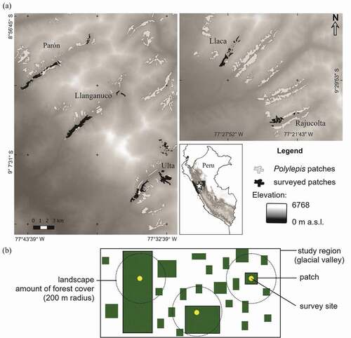
We selected 59 Polylepis patches ranging in size from 0.01 ha to 199 ha (mean ± SD = 13.9 ha ± 31.7), totalling 822 ha and distributed along the entire elevational gradient of each of our five glacial valleys (3,300 ̶ 4,700 masl) (Figures 2 and Figures 3). A patch of Polylepis forest was defined as a continuous woodland >30 m from any other patch [44,45]. Because Polylepis forests are easily distinguished from other plant communities in satellite images [47], we manually delimited the boundaries of each patch on images of 0.5 m-resolution from Google Earth [74]. The topographic complexity of the area prevented us from surveying patches located on cliffs or otherwise inaccessible areas. Forest patches were dominated by Polylepis albicans at lower elevations (3,300 ̶ 4,000 masl) or by P. weberbaueri at upper elevations (4,000 ̶ 4,700 masl), but a variety of trees and shrubs occurred within patches (see [72,75]).

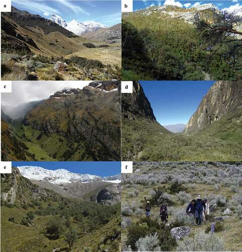
Figure 3. Examples of Polylepis forest from the glacial valleys of Ulta (a), Rajucolta (b), Llaca (c), Llanganuco (d) and Parón (e) within Cordillera Blanca. Matrix habitats are dominated by Puna grassland (a and e) or shrublands (f)

We defined our landscape as the area within a 200-m radius around each survey site (12.5 ha in area), in which we manually calculated the amount of Polylepis forest using the “Measure Area” tool of QGIS -v3.0-Girona [76] on the same Google Earth Pro [74] images (mean ± SD = 4.46 ha ± 3.88; range = 0 ̶ 12.5 ha). Although our landscapes were smaller than often used in other studies, the size was consistent with the relatively small scale of movements described for many of our study species [77,78]. Our landscape size also avoided problems with spatial autocorrelation of the amount of habitat among sites (sill = −10.3, range = 104,698 m, nugget = 12.1) (Figure S1).

Bird surveys

A robust sampling design for multiple species [79–81] was used to survey birds at 187 sites located within both forest (n = 140) and the matrix, which was comprised of Puna grassland or shrubland (n = 47). At each site, we used a GPS (GARMIN GPSMAP64) to record UTM coordinates and elevation (±10 m), the latter of which were highly correlated (r = 0.995) with the Advanced Spaceborne Thermal Emission and Reflection Radiometer (ASTER) – Global Digital Elevation Model v2 (GDEM2) of 30-m resolution [82]. Small patches contained only one site placed roughly in the center of the patch, but large patches contained up to 10 sites distributed throughout the patch and separated by ≥150 m (mean ± SD = 190 m ± 74.15; min – max = 150–480 m). Sites in the matrix were separated by > 200 m (245 ± 85.80; 200–650 m) and placed along the whole elevation gradient.

Surveys were conducted during the dry seasons (May to August) of 2014 and 2016 and the wet season (January to April) of 2015 by four trained observers. Each site was surveyed 3–13 times (mean ± SD = 7.57 ± 2.53) between sunrise (~0500 ̶ 0600 h) and 1200 h, totaling 1416 visits during which an observer recorded all birds seen or heard within 50 m over a 10-min period. Survey order and observers were changed across visits to avoid bias related to bird activity, time of day, or observer experience [44,45,72]. We excluded large raptors, aquatic birds, and birds identified only to genus.

Based upon published literature [41,44–47,64,83], each species was assigned to one of three habitat guilds: (1) Polylepis forest that includes (a)Polylepis forest specialist (species highly restricted to Polylepis ecosystem during most of their life-cycle by specific adaptations or behaviors that allows them to exploit specific Polylepis resources) and (b) Polylepis-associated species (species strongly associated with Polylepis forest during part of their life-cycle but facultatively able to exploit other ecosystems); (2) grassland Puna (species primarily associated with open areas dominated by grasslands such as Stipa or Calamagrostis spp.); or (3) shrubland (species primarily associated with shrublands composed of Baccharis spp., Berberis spp., Gynoxys spp., Weinmannia spp., Senecio spp., Lupinus spp. Brachyotum spp., among others). Birds of conservation concern (15 species) included Polylepis specialists (3 species) and Polylepis-associated species (8 species), endemics to Peru (10 species), and species included in The International Union for Conservation of Nature’s Red List of Threatened Species [50] (6 species) (Table S1).

Data analysis

Occupancy models and sensitivity to landscape attributes

We applied a multispecies occupancy model (MSOM) to our survey data [84–86]. This approach uses species-specific models of occurrence within a hierarchical (i.e., multilevel) framework, while accounting for heterogeneity in species detectability and habitat relationships [85–88]. MSOMs make inferences about the aggregated response of all modeled species in a community by specifying a common mean and variance hyperparameters for the occupancy and detection parameters for each species [86]. The method can incorporate the responses of rare species [85,88,89] and estimate species richness while accounting for species not detected during surveys [86,90,91]. By stacking the detection histories by year, we allowed the probabilities of occupancy and detectability to be modeled independently for each year while using a “single-season” occupancy model approach. This parameterization is an alternative to multiseason models where the parameters of colonization and extinction are unable to converge due to a limited number of observations (e.g. endemic and rare species) [92,93].

Species observations (y_i,j,k, of species i = 1,2, …, 88 at site j = 1,2, …, 561 (187 sites stacked in 3 years) during each survey k = 1,.,5) were modeled as imperfect observations of true occurrence states, z_i,j, given a certain detection probability, p_i,j,k. Detection was modeled as y_i,j,k│z_i,j ~ Bernoulli (z_i,j p_i,j,k), where z_i,j = 1 if species i was present at site j, or z_i,j = 0 if not. As elevation can modulate the effects of site covariates [94,95], we simultaneously estimated species-specific occupancy probabilities in function of linear, quadratic, and interactive relationships of elevation (ELV) with patch size (SIZE), and amount of Polylepis forest within a 200 m-radio (AMNT). The year effect was defined by two dummy variables, y2 and y3 that correspond to the second (2015) and third (2016) survey year. An initial full model (Eq. 1) was defined as:

logit(ψ_i,j) = β0_i + β1_i (ELV_j)+ β2_i (ELV_j²) + β3_i (SIZE_j) + β4_i (SIZE_j²) (Eq. 1)

+ β5_i (AMNT_j) +β6_i (AMNT_j²) + β7_i (ELV_j * SIZE_j) + β8_i (ELV_j * AMNT_j)

+ β9_i (SIZE_j * AMNT_j) + β10_i (ELV_j + SIZE_j * AMNT_j)

+ β11_i (y2_j) + β12_i (y3_j)

where β0_i was the species-specific intercept and first year (2014) effect, β1_i … β12_i where the species-specific occupancy model coefficients treated as random effects with a normal distribution of their hyperparameters μ and σ², such as β0_i, … β12_i ~ Normal(μ_{β0, …,} μ_β12, σ²_{β0, …,} σ²_β12). Coefficients β1, β3 and β5 represented the linear main effects of elevation, forest patch size and amount of forest for species i while coefficients β2, β4 and β6 were the main effects of the quadratic components, respectively. The coefficients β7, β8, and β9 represented the interactive effect of the three covatiates whereas β10 represent their full interaction. Parameters β11 and β12 are the second- and third-year effect respectively for each j site. Likewise, μ_{β0, …,} μ_β12 and σ²_{β0, …,} σ²_β12 were the mean and variance community responses (across species) to each covariate (e.g. μ_β3, σ²_β3 for forest patch size) [91]. Following the recommendations of Kéry and Royle [91] and Broms [93], we used uninformative priors for the mean (μ) and variance (σ²) of the hyper-parameters (e.g. normal distribution with mean zero and variance of 0.1 for the mean community response (μ), and uniform distribution with mean zero and variance of 5 for the community standard deviation (σ)). This initial model was later contrasted to a reduced model (Eq. 2) that did not include the interactive terms with elevation:

logit(ψ_i,j) = β0_i + β1_i (ELV_j) + β2_i (ELV_j²) + β3_i (SIZE_j) + β4_i (SIZE_j²) (Eq. 2)

+ β5_i (AMNT_j) +β6_i (AMNT_j²) + β7_i (SIZE_j * AMNT_j) + β8_i (y2_j) + β9_i (y3_j)

As our ability to detect the species could vary along the day and across open and forested sites; detectability was modeled for each species i using forest cover (COV), survey time (TIME; e.g., 06:30 h = 6.5) and survey year defined by the same two dummy variables, y2 and y3:

logit(p_i,j,k) = α0_i + α1_i * COV_j + α2_i * TIME_j,k + α3_i * y2_j + α4_i * y3_j(Eq. 3)

where α0_i, …, α4_i were the species-specific detectability model coefficients treated as random effects with a normal distribution of their hyperparameters μ and σ², that follow α0_i … α4_i ~ Normal(μ_{α0- α4}, σ²_{α0- α4}).

Models were run using JAGS [96] via R v 3.3.1 [97] and the “jagsUI” package v 1.4.4 [98]. We standardized all the continuous covariates (elev, p_size, a_for, forcov, time) around a mean of zero. For each analysis, we ran three parallel Markovian chains of 20,000 iterations, applying burn-in to the first 5,000 and thinning rate of 15, which left us with 3,000 samples to build the posterior distribution of the different parameters. Though a visual inspection of traceplots and using the Brooks-Gelman-Rubin (BGR [99],) convergence diagnostic value of Rhat <1.1 [100], we assessed the convergence of the results. Both, the full and reduced model were evaluated by comparing their respective DIC (Deviance Information Criterion [101];) values and by direct observations of their interactive effects. The model structure and model script are provided in Supplementary Information A and B.

Local species richness

The number of species expected to occur at each survey site was a derived community metric from the posterior draws of Markov Chain Monte Carlo (MCMC) runs. This allowed the incorporation of uncertainty of the parameters into the local species richness estimation that followed:

$N\mathrm{j}=\sum _{i=1}^{88}z\mathrm{i},\mathrm{j}(\mathrm{E}\mathrm{q}.4)$

where N_j is the total number of species occurring at site j from the true occurrence state z_i,j. Relationships between species richness and elevation, patch size and forest cover were then evaluated by simple ordinary least squares (OLS) regressions with lineal and quadratic components [89].

Cumulative species-area curve analysis

We discerned effects of patch size from amount of forest by estimating cumulative species richness and comparing slopes of species–area relationships among a set of samples ordered by ascending versus descending patch size while controlling for the cumulative amount of habitat surveyed (sensu Quinn and Harrison [31] and Fahrig [9]). “Cumulative forest area” referred to the consecutive sum of different Polylepis patches ordered from small to large and vice versa. The cumulative species–area curves associated with both ordering schemes were then constructed from the estimated species richness of each cumulative forest area [102]. The following relationships were possible: 1) species richness increases with patch size, such that a single large patch supports more species than several smaller patches of equal cumulative area (Figure 4(a)); 2) species richness declines with increasing patch size, where smaller patches contain more species than a large patch whose area is equal to the sum of the smaller patches (Figure 4(b)); or 3) no association with patch size; instead species richness increases with total area of habitat, irrespective of the number of patches and therefore, both curves overlaps (Figure 4(c)). A positive response to patch size was indicated by a steeper cumulative species-area curve when patches were ordered from large to small versus when ordered from small to large (Figure 4(a)), whereas the opposite pattern indicated a negative response. Similar slopes were interpreted to indicate lack of evidence for a meaningful response to patch size [8] (Figure 4(c)).

Figure 4. Contrasting predictions based on cumulative species-area curves, including (a) a positive association with patch size (i.e., samples in larger patches, while controlling for surveyed area, have more species), (b) negative association with patch size (i.e., more species in smaller patches), or (c) no association with patch size

Although our MSOM facilitates estimating local species richness at each site, it does not allow to estimate cumulative species–area curves because species identities were not retained. Therefore, we estimated species richness using the R package “iNEXT” (iNterpolation and EXTrapolation), a new-unbiased species richness estimator based on Hill numbers and sample completeness that retains species identity [103–105]. The calculation was based upon an abundance matrix, Y ≡ {y_ij, i, j} where i represents each of the observed (S_obs) and unobserved (S_DA) species during the study on j = 1, …, J cumulative forest area (Figure S2). Given that multiple (x= 1, … 10) sites were surveyed k = 3, … 5 times on each patch, y_ij is the consecutive sum of different species observations after k visits to x surveys sites. Then, y_ij ≥1 when species i was detected in any of the k visits at survey site x within the j cumulative forest area and y_ij = 0 when it was not detected at all [104].

Results

In total, 13,780 observations of 100 bird species were registered, although only 13,210 observations of 88 bird species were included in the analysis after removing raptors, aquatic birds, and birds identified only to genus (Table S2). Over the three seasons of sampling, 13 of the 15 species of conservation concern had at least 30 detections: Xenodacnis parina (Tit-like Dacnis; 900 observation at 164 different sites), Scytalopus affinis (Ancash Tapaculo, endemic; 404, 146), Cranioleuca baroni (Baron’s Spinetail, endemic; 386, 134), Metallura phoebe (Black Metaltail, endemic; 294, 114), Grallaria andicolus (Stripe-headed Antpitta; 261, 114), Leptasthenura pileata (Rusty-crowned tit-spinetail, endemic; 230, 103), Atlapetes rufigenis (Rufous-eared Brushfinch, endemic, NT; 228, 100), Geocerthia serrana (Striated Earthcreeper, endemic; 181, 95), Conirostrum binghami (Giant Conebill, NT; 158, 80), Leptasthenura yanacensis (Tawny Tit-Spinetail, NT; 105, 41), Zaratornis stresemanni (White-cheeked cotinga, endemic, VU; 104, 41), Microspingus alticola (Plain-tailed Warbling-Finch, endemic, EN; 67, 49), Anairetes alpinus (Ash-breasted tit-tyrant, EN; 32, 15). Conclusions are based on our reduced MSOM model, which received the strongest support (Full Model: pD = 46,894.6 and DIC = 76,089.87; Reduced Model: pD = 18,757.6 and DIC = 47,643.52) and lacked significant interactive effects among elevation, patch size and amount of forest (Figure S3, Figure S6).

In general, the High-Andean bird community of Cordillera Blanca was characterized by many rare, but only a few common species (e.g. Tit-like Dacnis). Avian occurrence and detectability, though variable across species, were usually low each year (Occurrence: mean ± SD = 0.24 ± 0.05, range = 0.01 ̶ 0.89; detectability: mean ± SD = 0.06 ± 0.001, range = 0.1 ̶ 0.64) (Figure S2.4.). Some species were nearly ubiquitous and easily detected across years (e.g. Xenodacnis parina, psi = 0.80, p= 0.63); others were rare and difficult to detect when present (e.g. Anairetes alpinus, psi = 0.09, p= 0.31) despite being consistently observed in the same few sites (outside of the point count period) among multiple years.

Species richness and community response

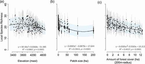
The estimated number of species occurring at each site slightly differed among years (Figure S5), yet only year 3 had a significant effect with respect to the first year (Table 1; μ_α4 (95% PI) = −0.32 (−0.56, −0.1)). Local species richness slightly peaked at mid-elevation (~3,800 m) and declined with forest patch size and amount of Polylepis forest in the landscape independently of the year (Figure 5). Estimated number of species at a site was 19 species (range = 13 ̶ 28) in year one, 22 (14 ̶ 35) in year two, and 23 (13 ̶ 34) in year three. Some of the highest estimates corresponded to sites at ~4,000 m, within fragments under 50 ha or in landscapes with less than 50% of forest cover.

Table 1. Community-level hyper-parameters for occupancy and detection in relation to elevation, patch size and amount of forest area. Each value represents the mean, standard deviation, and the 95% posterior interval of the effect of each parameter on the whole bird community. Rhat is the Brooks-Gelman-Rubin (BGR) measure of convergence of the three Markovian chains. Rhat <1.1 indicate convergence. These parameters correspond to our reduced model

Community-level hyper-parameter		Mean	Standard deviation	95% Posterior Intervals	Rhat
μβ0	Mean intercept	−2.08	0.29	−2.65 - −1.51	1.01
σβ0	SD of intercept	2.32	0.23	1.91 - 2.79	1.00
μβ1	Elevation (lineal term)	−0.51	0.18	−0.84 - −0.17	1.00
σβ1	Elevation (lineal term)	1.46	0.15	1.19 - 1.78	1.01
μβ2	Elevation (quadratic term)	−0.22	0.07	−0.36 - −0.09	1.00
σβ2	Elevation (quadratic term)	0.43	0.07	0.31 - 0.57	1.00
μβ3	Patch Size (lineal term)	0.05	0.15	−0.22 - 0.36	1.10
σβ3	Patch Size (lineal term)	0.26	0.14	0.03 - 0.54	1.07
μβ4	Patch Size (quadratic term)	0.03	0.09	−0.15 - 0.2	1.35
σβ4	Patch Size (quadratic term)	0.06	0.04	0 - 0.15	1.01
μβ5	Amount of Area (lineal term)	−0.3	0.12	−0.54 - −0.06	1.13
σβ5	Amount of Area (lineal term)	0.72	0.09	0.56 - 0.91	1.00
μβ6	Amount of Area (quadratic term)	−0.02	0.09	−0.18 - 0.15	1.34
σβ6	Amount of Area (quadratic term)	0.16	0.08	0.02 - 0.3	1.04
μβ7	Patch Size * Amount of Area	−0.17	0.22	−0.55 - 0.22	1.45
σβ7	Patch Size * Amount of Area	0.08	0.06	0 - 0.22	1.01
μβ8	Year 2	0.41	0.14	0.13 - 0.67	1.00
σβ8	Year 2	0.7	0.14	0.43 - 0.99	1.02
μβ9	Year 3	0.39	0.23	−0.04 - 0.84	1.00
σβ9	Year 3	1.46	0.2	1.09 - 1.89	1.00
μα0	Mean intercept	−1.88	0.17	−2.22 - −1.56	1.03
σα0	SD of intercept	1.07	0.13	0.83 - 1.36	1.02
μα1	Forest cover	−0.22	0.05	−0.33 - −0.11	1.00
σα1	Forest cover	0.38	0.05	0.3 - 0.49	1.00
μα2	Survey time	−0.09	0.03	−0.14 - −0.03	1.00
σα2	Survey time	0.15	0.03	0.1 - 0.21	1.00
μα3	Year 2	−0.03	0.11	−0.24 - 0.17	1.00
σα3	Year 2	0.58	0.1	0.4 - 0.8	1.03
μα4	Year 3	−0.32	0.12	−0.56 - −0.1	1.00
σα4	Year 3	0.53	0.12	0.31 - 0.79	1.02

Figure 5. Average (among three years) local species richness (alpha diversity) at each site (n=187) declines with increasing elevation (a), patch size (b) and amount of Polylepis forest within 200 m-radio (c). Black dots and vertical lines represent the average mean and 95% posterior intervals of the species richness estimated through MSOM for each site. The solid black and shade areas represent the mean ± 95% CI of lineal regressions

Avian composition within Polylepis forests contrasted sharply with the comparatively more homogeneous composition of Puna and shrubland landscape matrix (Figure 6). Polylepis forests were dominated by forest-associated species (~70%, especially aerial (55%) and terrestrial (26.4%) insectivores) and species of conservation concern (~60%), irrespective of forest patch size (Figure 6(a,c,e,f)). In contrast, most species detected within the matrix were species associated to Puna (29.4% of species detected) and shrublands (28%) although species associated with forest (42.6%) were surprisingly common (Figure 6(a)). Foraging guilds in the matrix were dominated by aerial insectivores (37.6%), terrestrial insectivores (29.4%), and granivores (22%) (Figure 6(c,d)).

Figure 6. Avian community composition across five different categories of patch size and amount of forest cover within the landscape. The community was classified according to (1) habitat associations (a, b), (2) five foraging guilds (c, d), and (3) status of conservation priority (e, f). The total numbers of observations during the three years on each category are in parenthesis over each bar (this applies to the other two graphs below)

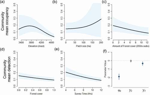
Mean occupancy for the entire High-Andean bird community peaked around 3,800 m (Figure 7(a)) (linear component: μβ₁ (95% PI) = −0.51 (−0.84, −0.17); quadratic component: μβ₂ (95% PI) = −0.22 (−0.36, −0.09)). Mean community occupancy increased with patch size (Figure 7(b)) (linear component: μβ₃ (95% PI) = 0.05 (−0.22, 0.36); quadratic component: μβ₄ (95% PI) = 0.03 (−0.15, 0.2) but declined with the amount of Polylepis forest in the landscape (Figure 7(c)) (linear component: μβ₅ (95% PI) = −0.3 (−0.54, −0.06)) (Table 1). Overall, our estimates of bird community occupancy and detectability were comparable across years (Figure S3), though there was some variability related to effect sizes among years. Notably, patch size was significant in year two (μβ₈ (95% PI) = 0.41 (0.13, 0.67) but not year three (μβ₉ (95% PI) = 0.39 (−0.04, 0.84). Detection probability declined slightly with forest cover (Figure 7(d)) (μα₁ (95% PI) = −0.22 (−0.33, −0.11), over the course of a day (μα₂ (95% PI) = −0.09 (−0.14, −0.03)) (Figure 7(e)), and in year three (2016) (Figure 7(f); μα₄ (95% PI) = −0.32 (−0.56, −0.1)).

Figure 7. Mean community occupancy for birds in the High Andes was highest at mid-to-low elevations (a), in large forest patches (b) and in local landscapes with relatively low forest cover (c) while accounting for detectability per year (d,e,f). Shade areas represent the 95% of posterior intervals. Parameters y₂ and y₃ correspond to second- and third-year effect with respect to the initial year (α₀) (f)

Sensitivity of individual species

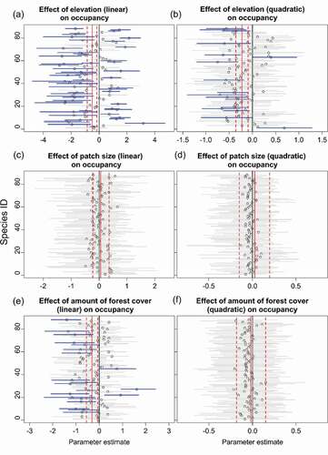
Occupancy probability for 63 of 88 bird species was significantly associated with elevation (46 linear and 17 quadratic relationships) (Figure 8(a,b); Table S1; Figure S7). Size of Polylepis patches was not significantly related to occupancy of any bird species (Figure 8(c–d). Forest cover within 200-m was negatively related to 18 species and positively to three species (Figure 8(e); Figure S7). Sixteen species that declined with increasing amount of forest were generalists or species that use shrubland or Puna habitats (Table S2; Supplementary Information B) whereas two of the three that responded positively were species of conservation concern that primarily forage in Polylepis trunks (the near-threatened Giant Conebill and endemic Baron’s Spinetail). No species responded quadratically to the amount of forest or the interaction of patch size and amount of forest (Figure 8(f); Figure S7).

Figure 8. Species- and community- level responses to elevation (a-b), patch size (c-d) and amount of Polylepis forest cover in the landscape (e-f). Open dots represent the species-specific mean response. Horizontal lines represent the 95% posterior intervals. Intervals that do not overlap zero (blue lines) indicate that estimated coefficients differed significantly from zero, indicating an effect of the parameter. Solid and dashed vertical lines (red) are the mean and 95% PI of the community response, respectively. Species ID correspond those in Table S1

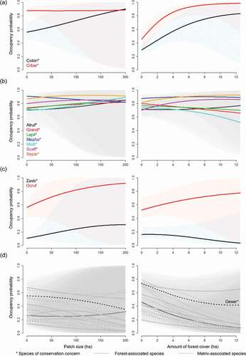
Our four predictions of relationships with patch size and forest cover captured all species-specific occurrence profiles (Figures 1 andFigures 9). Occupancy of Giant Conebill and Baron’s Spinetail were negatively related to forest cover (Figure 9(a)). In contrast, neither patch size nor forest cover were related to seven other Polylepis-associated species of conservation concern (Rufous-eared Brushfinch, Stripe-headed Antpitta, Rusty-crowned tit-spinetail, Black Metaltail, Plain-tailed Warbling-Finch, Ancash Tapaculo, Tit-like Dacnis) (Figure 9(b)). Occurrence of only one species of conservation concern (White-cheeked Cotinga) along with one widespread and common Andean bird (Rufous-breasted Chat-tyrant) increased with patch size (Figure 9(c)). Most Puna species, including one species of conservation concern (Striated Earthcreeper), were more likely to occur in smaller patches and in areas with less forest cover (Figure 9(d)). Finally, no threshold effects (a faster reduction) were observed for any bird species.

Figure 9. Mean species occupancy probabilities in response to Polylepis patch size (left in a,b,c,d) and amount of forest cover (%) within 200-m radio (right in a,b,c,d). The solid lines and shade areas represent the mean ± 95% Posterior Intervals of the reduced MSOM. Cobin = Giant Conebill, Crbar = Baron’s Spinetail, Atruf = Rufous-eared Brushfinch, Grand = Stripe-headed Antpitta, Lepil = Rusty-crowned tit-spinetail, Mepho = Black Metaltail, Mialt = Plain-tailed Warbling-Finch, Scaff = Ancash Tapaculo, Xepar = Tit-like Dacnis, Zastr = White-cheeked Cotinga, Ocruf = Rufous-breasted Chat-tyrant, Geser = Striated Earthcreeper. Individual plots of the 88 species are in Figure S7

Cumulative species-area curves

Cumulative species-area curves suggested a negative association between species richness and patch size overall, and for forest and shrubland birds in particular (Figure 10), such that greater numbers of species were detected in smaller than larger patches. No clear pattern was detected for species associated with Puna grasslands (Figure 10(c)). Notably, however, the two curves (LS and SL) overlapped in all cases with ~400 – 600 ha of cumulative forest cover, suggesting that birds were less sensitive to patch size in landscapes with comparably more forest.

Figure 10. Species richness estimation across both orders (large to small and vise-versa) of cumulative forest area of 59 Polylepis surveyed patches for all (a), forest (b), grassland Puna (c) and shrubland (d) species. Shade lines correspond to the 95% confidence interval

Discussion

We examined the extent to which patch size and amount of Polylepis forest within 200-m were related to occurrence of High-Andean birds across an elevation gradient (3,300–4,700 masl). Overall, the patterns we detected at both community and species levels were consistent with the hypothesis that many High-Andean birds, especially Polylepis specialists and Polylepis-associated species, are adapted to naturally patchy landscapes. Specifically, we found that most species responded more strongly to the amount of habitat (forest cover) than fragmentation per se, as indicated by patch size, or showed no response to patch and landscape characteristics. These results contrast with decades of research from heavily forested systems in temperate and lowland tropical regions, in which researchers have documented harmful consequences of fragmentation to species that are habitat specialists, range-restricted, sensitive to disturbance, have low vagility, and/or occur within small populations [106-108] Yet despite possessing many traits that are typically associated with vulnerability to fragmentation, most Polylepis-Puna species seemed relatively insensitive to changes in landscape configuration, like forest patch size, and were able to exploit small or remnant patches as long as sufficient forest remained within the landscape.

High-Andes species richness and composition

Avian species richness within our patchy system was greatest within small fragments and in landscapes with comparably low amount of forest cover (and therefore more isolation [5],) (Figure 5). This finding is consistent with Lloyd’s report [44] from Cuzco, where species richness was comparable across large, medium and small patches but is in opposition with Tinoco’s et al. [109], results from Ecuador, where forest area had a positive relationship with species richness. Although inconsistent with predictions from Theory of Island Biogeography, where the number of species in a fragment is defined in terms of patch size and isolation [110], our results underscore the importance of matrix attributes [12,111], patch quality [112], and amount of habitat [8,11] in terrestrial systems where the matrix is not considered to be “inhospitable” but instead can strongly shape community organization and structure [113,114].

In the High Andes, Puna and shrubland habitats were used by many High-Andean birds that also use Polylepis forests to some extent [44,71,107]. Notable, Gynoxys plants seems to play an important role in the Polylepis landscapes of Ecuador [109,115]. In this way, matrix attributes should modulate the degree of connectivity among fragments, influence the nature of the edge effects, and be the source of not only many opportunistic and generalist species, but also forest-associated species (e.g. Tit-like Dacnis). Seasonal changes in structural and environmental conditions could also influence the composition of the bird community along the elevation, probably by modifying the habitat quality for different species [68]. Structural characteristics, such as DBH, tree height, canopy cover, mosses cover, seems to be especially important in our study site, whereas seasonal responses may depend on bird species traits [72]. Further studies should consider that the influence of matrix may change with latitude based on climatic and floristic conditions [109], modulating the effect of patch size across the Andes [112,115].

The importance of the total amount of Polylepis forest

Species occurrence was better explained by the total amount of Polylepis forest within 200 m than patch size, though we recognize that species did not uniformly show this pattern (Figures 8 and Figures 9). For example, we estimate occupancy probability of the Giant Conebill should decline by roughly half (0.54, with a range from 0.83 to 0.29) given a loss of 90% of forest within the landscape, but only by 0.34 (from 0.90 to 0.56) when patch size is reduced from 200 to 1 ha (Figure 9(a,b)). Likewise, occupancy by Baron’s Spinetail, a Polylepis-associated species, would be expected to decline by half to similar losses of forest cover but show little response to changes in patch size. Despite some variation among species, our results suggest that habitat loss would have more severe consequences for these species than habitat fragmentation, as indicated by patch size. In addition to our hypothesis that High-Andean birds are adapted to patchy landscapes, we suggest two additional contributors to the patterns we describe. First, the specific habitat features required by many Polylepis specialists and Polylepis-associated species are likely to be a function of the amount and quality of forest rather than patch size only [44,72,77]. Second, many Polylepis specialists readily use matrix habitats and the resources they provide [72,109,115].

Our failure to detect strong responses to patch size is unlikely to be an artifact of working within intact or heavily forested landscapes as non-interaction between patch size and amount of forest cover was found. Previous research shows that the effects of patch size and isolation usually manifest when less than ~30% of habitat remains in a landscape [11]. Throughout most of the Andes, Polylepis woodlands comprise less than 30–20% of land cover (see [56]), with 8–23% cover in our study region in Cordillera Blanca (Table 2). Another source of bias could be paucity of detections for certain species along the range of patch size and amount of forest. However, our results are more precise for small patches as uncertainty increase with patch size and forest cover (Figure 9). In this way, our findings are consistent with the Habitat Amount Hypothesis (HAH), which posits that habitat availability is more important than spatial configuration [8], and the idea that many High-Andean birds ̶ specialized or highly associated to Polylepis forest ̶ are adapted to this patchy landscape configurations.

Table 2. Proportion of forest cover with respect to the landscape extension of each of the five glacier valleys studied in Cordillera Blanca, Peru. The landscape extension was delimitated by the natural entrance of the valleys and the 5,000 m elevational line and calculated based on a Digital Elevation Model. The forest cover was calculated in the same way as the studied patches

Glacier Valleys	Landscape (ha)	Forest Cover (ha)	Proportion
Paron	3468.32	581.22	16.76
Llanganuco	5177.21	555.17	10.72
Ulta	4509.15	926.4	20.54
Llaca	625.34	140.15	22.41
Rajucolta	2578.67	228.47	8.86

The importance of small Polylepis patches

Most conservation and restoration efforts place high value on large Polylepis forests, sometimes to the exclusion of small fragments [44,45,72,77], but our results challenge this assumption. Rather, we provide a striking illustration of the ability of many Polylepis specialist to use very small Polylepis fragments (<1 ha). In fact, small patches of Polylepis forest in the Cordillera Blanca were as likely to be used as large patches by seven Polylepis-associated species of conservation concern, including the endangered and endemic Plain-tailed Warbling-Finch (Figure 9).

The weak signal for patch size may reflect the fact that small patches often contain habitat features required by certain specialists, or in other cases, that some species prefer or regularly use habitat edges. The Tawny Tit-Spinetail, for which 56% of records were in fragments smaller than 6 ha (mean patch size ± SD = 1.71 ha ± 2.07), provides an example of the former, as the species requires undisturbed forest with tall or mature Polylepis trees, rich in mosses cover and steep rocky terrain at high elevations (>4000 m) [45,71,72]. On the other hand, a preference for habitat edges may explain why Ash-breasted Tit-tyrant occurred either within small patches (mean patch size ± SD = 2.34 ha ± 2.3, range = 0.046 ̶ 5.6 ha) or along the irregular edge of a large forest patch (mean patch size ± SD = 47.7 ha ± 14.76, range = 17.6 ̶ 53.77 ha; Figure 3(a-b)).

Small Polylepis fragments also can be used as secondary habitats, as suggested by our observations that some Polylepis specialists patrol (individually, in flocks, or in multispecies flocks) several small patches for specific resources (e.g. insects, flowers and fruits), probably as part of their home ranges. We observed patrolling behavior for the Giant Conebill, the Rufous-eared Brushfinch, the Baron’s Spinetail, Rusty-crowned Tit-Spinetail, Plain-tailed Warbling-Finch and the White-cheeked Cotinga [68,72]. Certainly, the home ranges of some Polylepis specialist are composed of multiple patches, including small ones, that are visited routinely everyday [78,115]. Our finding that small Polylepis patches are important habitats for multiple High-Andes species of conservation concern signals another potential risk given that small patches may be most vulnerable to loss or degradation [116,117].

Conservation implications

Although many others have studied the relative importance of landscape configuration versus composition [67,118–120], we believe ours is the first to explicitly test these differences in a high tropical mountain system. We recognize that fragmentation negatively impacts biodiversity and drives species loss in many systems [4,11,22,121,122], but we show here that patchy landscapes and small patches can contribute to biodiversity conservation [9,28,102,123]. Our work has three central implications for conservation.

First, conservation efforts should focus most heavily on avoiding loss of Polylepis forest rather than on avoiding fragmentation per se. Although landscape configuration is important in some contexts [11,124] and for some species [67,125], birds in our system responded more strongly to forest cover than patch size. That said, we caution that fragmentation might promote species richness in small fragments by increasing the abundance of generalist and matrix-associated species that might conceivably displace other species of conservation concern or have other negative outcomes [4,126].

Second, small patches of Polylepis seem to contribute as much to conservation as large fragments, given the same amount of forest within the landscape. Even the loss of small fragments can have potentially serious consequences, especially if they contain special habitat features absent in larger fragments [44–46,72,77,109]. As first noted by Fjeldså [127] the persistence of many Polylepis specialists in small and isolated Polylepis forest is no less than remarkable. Our study reinforces this observation and further provides evidence that many Polylepis species are adapted to patchiness. Therefore, conserving, restoring, and creating many more small and scattered patches of Polylepis should be considered by practitioners and decision-makers.

Third, attributes of the landscape matrix play important roles in structuring Andean bird communities [72,109,115]. Specifically, a more heterogeneous matrix (e.g shrublands) is known to enhance connectivity and bird movements [109,115]. Plant species like Gynoxys, Baccharis, Buddleia, Lupinus among others, should be included in matrix restoration projects as many bird species seems to depend on the diversity of resources that they provide (e.g. nectar, insects, fruits).

Author contribution

CSSR conceived and designed the study. AR provided advise during the whole process. CSSR analyzed the data and wrote the first draft of the manuscript. CSSR and AR reviewed and improved the manuscript.

Acknowledgments

This research was funded by FONDECYT-CONCYTEC (Nº 237-2015-FONDECYT). We are also grateful to the Fulbright Scholarship and support from Cornell University that supported CSSR during his graduate studies. We also deeply appreciate financial support provided by Cornell Lab of Ornithology, the Athena Grant, the Bergstrom Award of the Association of Field Ornithologists as well as the American Alpine Club Research Grants 2017. Thanks to Jessica Pisconte, Nathaniel Young, Rosaura Watanabe, Nicolas Mamani, Julio Salvador, Celia Sierra and James Purcell for being the core field crew for data gathering and data entry; to the Huascaran National Park staffing, Ing. Jesús Gómez, Selwyn Valverde, Martín Salvador, and Oswaldo Gonzales for facilitating permits; as well as to many park rangers that granted access and helped in different ways. We thank to André Dhondt, Stephen Morreale, Viviana Ruíz-Gutiérrez, Wesley M. Hochachka, Lynn Marie Johnson and Laura Morales for comments, recommendations and guidance that helped to improve this manuscript.

Disclosure statement

No potential conflict of interest was reported by the authors.

Supplementary material

Supplemental data for this article can be accessed here

Additional information

Funding

This work was supported by the American Alpine Club [2017]; the E. Alexander Bergstrom Memorial Research Award of the Association of Field Ornithologists [2015]; FONDECYT [237-2015]; Cornell Lab of Ornithology - Athena Fund [2014,2015,2016].

References

- Fahrig L. Relative effects of habitat loss and fragmentation on population extinction. J Wildl Manage. 1997;61:603–610.
- Fahrig L. Effect of habitat fragmentation on the extinction threshold: a synthesis. Ecol Appl. 2002;12(2):346–353.
- Lindenmayer DB, Franklin JF. Conserving forest biodiversity: a comprehensive multiscaled approach. Island press; Washington, DC. USA. 2002.
- Haddad NM, Brudvig LA, Clobert J, et al. Habitat fragmentation and its lasting impact on Earth’s ecosystems. Sci Adv. 2015;1(2):e1500052.
- Fahrig L. Effects of habitat fragmentation on biodiversity. Annu Rev Ecol Evol Syst. 2003;34(1):487–515.
- Wiegand T, Revilla E, Moloney KA. Effects of habitat loss and fragmentation on population dynamics. Conserv Biol. 2005;19(1):108–121.
- Liu J, Wilson M, Hu G, et al. How does habitat fragmentation affect the biodiversity and ecosystem functioning relationship? Landscape Ecol. 2018;33(3):341–352.
- Fahrig L, Triantis K. Rethinking patch size and isolation effects: the habitat amount hypothesis. J Biogeograph. 2013;40(9):1649–1663.
- Fahrig L. Ecological responses to habitat fragmentation per se. Annu Rev Ecol Evol Syst. 2017;48:1–23.
- McGarigal K, Cushman SA. Comparative evaluation of experimental approaches to the study of habitat fragmentation effects. Ecol Appl. 2002;12(2):335–345.
- Andrén H. Effects of habitat fragmentation on birds and mammals in landscapes with different proportions of suitable habitat: a review. Oikos. 1994;71:355–366.
- Rodewald AD, Yahner RH. Influence of landscape composition on avian community structure and associated mechanisms. Ecology. 2001;82(12):3493–3504.
- Yaacobi G, Ziv Y, Rosenzweig ML. Habitat fragmentation may not matter to species diversity. Proc R Soc London B: Biol Sci. 2007;274(1624):2409–2412.
- Bissonette JA, Storch I. Landscape ecology and resource management: linking theory with practice. Island Press; Washington, DC. USA. 2002.
- Collinge SK. Ecology of fragmented landscapes. JHU Press; Baltimore. USA. 2009.
- Kareiva P. Habitat fragmentation and the stability of predator–prey interactions. Nature. 1987;326(6111):388.
- Lomolino MV. Body size evolution in insular vertebrates: generality of the island rule. J Biogeograph. 2005;32(10):1683–1699.
- Ferraz G, Nichols JD, Hines JE, et al. A large-scale deforestation experiment: effects of patch area and isolation on Amazon birds. Science. 2007;315(5809):238–241.
- Duckworth RA, Kruuk LE. Evolution of genetic integration between dispersal and colonization ability in a bird. Evolution. 2009;63(4):968–977.
- Cote J, Clobert J, Brodin T, et al. Personality-dependent dispersal: characterization, ontogeny and consequences for spatially structured populations. Philos Trans R Soc B. 2010;365(1560):4065–4076.
- Radford JQ, Bennett AF, Cheers GJ. Landscape-level thresholds of habitat cover for woodland-dependent birds. Biol Conserv. 2005;124(3):317–337.
- Fletcher JR, Didham J, Banks-Leite RK, et al. Is habitat fragmentation good for biodiversity? Biol Conserv. 2018;226:9–15.
- Sih A, Jonsson BG, Luikart G. Habitat loss: ecological, evolutionary and genetic consequences. Trends Ecol Evol. 2000;15(4):132–134.
- Gaggiotti OE, Hanski I. Mechanisms of population extinction. In: Hanski I, Gaggiotti OE, editors. Ecology, genetics and evolution of metapopulations. Finland; Academic Press; 2004. p. 337–366.
- Huffaker C. Experimental studies on predation: dispersion factors and predator-prey oscillations. Hilgardia. 1958;27(14):343–383.
- Hastings A. Spatial heterogeneity and the stability of predator-prey systems. Theor Popul Biol. 1977;12(1):37–48.
- Grez A, Zaviezo T, Tischendorf L, et al. A transient, positive effect of habitat fragmentation on insect population densities. Oecologia. 2004;141(3):444–451.
- Ethier K, Fahrig L. Positive effects of forest fragmentation, independent of forest amount, on bat abundance in eastern Ontario, Canada. Landscape Ecol. 2011;26(6):865–876.
- Holzschuh A, Steffan-Dewenter I, Tscharntke T. How do landscape composition and configuration, organic farming and fallow strips affect the diversity of bees, wasps and their parasitoids? J Anim Ecol. 2010;79(2):491–500.
- Saura S, Bodin Ö, Fortin MJ. EDITOR’S CHOICE: stepping stones are crucial for species’ long‐distance dispersal and range expansion through habitat networks. J Appl Ecol. 2014;51(1):171–182.
- Quinn JF, Harrison SP. Effects of habitat fragmentation and isolation on species richness: evidence from biogeographic patterns. Oecologia. 1988;75(1):132–140.
- Tscharntke T, Steffan-Dewenter I, Kruess A, et al. Characteristics of insect populations on habitat fragments: a mini review. Ecol Res. 2002;17(2):229–239.
- Klingbeil BT, Willig MR. Guild‐specific responses of bats to landscape composition and configuration in fragmented Amazonian rainforest. J Appl Ecol. 2009;46(1):203–213.
- Henden JA, Ims RA, Yoccoz NG, et al. Declining willow ptarmigan populations: the role of habitat structure and community dynamics. Basic Appl Ecol. 2011;12(5):413–422.
- Proctor J, Woodell SR. The ecology of serpentine soils. Adv Ecol Res. Academic Press 1975;9:255–366.
- Nyström M, Folke C. Spatial resilience of coral reefs. Ecosystems. 2001;4(5):406–417.
- Fine PV, García-Villacorta R, Pitman NC, et al. A floristic study of the white-sand forests of Peru. Ann Missouri Bot Garden. 2010;97(3):283–305.
- Pennington RT, Lehmann CE, Rowland LM. Tropical savannas and dry forests. Curr Biol. 2018;28(9):R541–R545.
- Simpson BB. A revision of the genus Polylepis (Rosaceae: sanguisorbeae). Smithsonian Contribut Bot. 1979;43:1–62.
- Gareca EE, Hermy M, Fjeldså J, et al. Polylepis woodland remnants as biodiversity islands in the Bolivian high Andes. Biodivers Conservat. 2010;19(12):3327–3346.
- Fjeldså J. Biogeographic patterns and evolution of the avifauna of relict high-attitude woodlands of the Andes. Steenstrupia. 1992;18(2):9–62.
- Fjeldså J. Polylepis forests - Vestiges of a vanishing ecosystem in the Andes. Ecotropica. 2002;8:111–123.
- Kessler M. Bosques de Polylepis. En: Botánica económica de los Andes centrales. Morales M, Ollgaard B, Kvist LP, Borchsenius F & Balslev H. Universidad Mayor de San Andrés, La Paz, 2006. p. 11.
- Lloyd H. Abundance and patterns of rarity of Polylepis birds in the Cordillera Vilcanota, southern Perú: implications for habitat management strategies. Bird Conserv Int. 2008;18(2):164–180.
- Lloyd H. Influence of within‐patch habitat quality on high‐Andean Polylepis bird abundance. Ibis. 2008;150(4):735–745.
- Lloyd H. Foraging ecology of high Andean insectivorous birds in remnant Polylepis forest patches. Wilson J Ornithol. 2008;120(3):531–544.
- Sevillano-Ríos CS, Rodewald A, Morales L. Ecología y conservación de las aves asociadas con Polylepis: qué sabemos de esta comunidad cada vez más vulnerable. Ecología Austral. 2018;28:216–228.
- Kessler M. The “Polylepis problem”: where do we stand. Ecotropica. 2002;8(2):97–110.
- Gosling WD, Hanselman JA, Knox C, et al. Long‐term drivers of change in Polylepis woodland distribution in the central Andes. J Veg Sci. 2009;20(6):1041–1052.
- IUCN 2018. The IUCN Red List of Threatened Species. Version 2018–2. http://www.iucnredlist.org Accesed on Nov 15th 2018.
- van der Hammen T. The Pleistocene changes of vegetation and climate in tropical South America. J Biogeograph. 1974;1:3–26.
- Pirie MD, Chatrou LW, Mols JB, et al. ‘Andean‐centred’genera in the short-branch clade of Annonaceae: testing biogeographical hypotheses using phylogeny reconstruction and molecular dating. J Biogeograph. 2006;33(1):31–46.
- Hughes C, Eastwood R. Island radiation on a continental scale: exceptional rates of plant diversification after uplift of the Andes. Proc Nat Acad Sci. 2006;103(27):10334–10339.
- Schmidt‐Lebuhn AN, Fuchs J, Hertel D, et al. An Andean radiation: polyploidy in the tree genus Polylepis (Rosaceae, Sanguisorbeae). Plant Biol. 2010;12(6):917–926.
- Hanselman JA, Bush MB, Gosling WD, et al. A 370,000-year record of vegetation and fire history around Lake Titicaca (Bolivia/Peru). Palaeogeograph Palaeoclimatol Palaeoecol. 2011;305(1–4):201–214.
- Valencia BG, Bush MB, Coe AL, et al. Polylepis woodland dynamics during the last 20,000 years. J Biogeograph. 2018;45:1019–1030.
- Chepstow-Lusty A, Bush MB, Frogley MR, et al. Vegetation and climate change on the Bolivian Altiplano between 108,000 and 18,000 yr ago. Quat Res. 2005;63(1):90–98.
- Weng C, Bush MB, Curtis JH, et al. Deglaciation and Holocene climate change in the western Peruvian Andes. Quat Res. 2006;66(1):87–96.
- Williams JJ, Gosling WD, Brooks SJ, et al. Vegetation, climate and fire in the eastern Andes (Bolivia) during the last 18,000 years. Palaeogeograph Palaeoclimatol Palaeoecol. 2011;312(1–2):115–126.
- Rodríguez F, Behling H. Late Quaternary vegetation, climate and fire dynamics, and evidence of early to mid-Holocene Polylepis forests in the Jimbura region of the southernmost Ecuadorian Andes. Palaeogeograph Palaeoclimatol Palaeoecol. 2012;350:247–257.
- Renison D, Cingolani AM, Suarez R. Efectos del fuego sobre un bosquecillo de Polylepis australis (Rosaceae) en las montañas de Córdoba, Argentina. Rev Chil Hist Nat. 2002;75:719–727.
- Purcell J, Brelsford A. Reassessing the causes of decline of Polylepis, a tropical subalpine forest. Ecotropica. 2004;10:155–158.
- Cingolani AM, Vaieretti MV, Giorgis MA, et al. Can livestock and fires convert the sub-tropical mountain rangelands of central Argentina into a rocky desert? Rangeland J. 2013;35:285–297.
- Fjeldså J, Krabbe N. Birds of the High Andes. University of Copenhagen: Zoological Museum; 1990.
- Sylvester SP, Sylvester MD, Kessler M. Inaccessible ledges as refuges for the natural vegetation of the high Andes. J Veg Sci. 2014;25(5):1225–1234.
- Sylvester SP, Heitkamp F, Sylvester MD, et al. Relict high-Andean ecosystems challenge our concepts of naturalness and human impact. Sci Rep. 2017;7(1):333467.
- Valente JJ, Betts MG, Albright T. Response to fragmentation by avian communities is mediated by species traits. Diversity Distrib. 2019;25(1):48–60.
- Sevillano- Ríos CS. Diversity, ecology, and conservation of bird communities of Polylepis Woodlands in The Northern Andes of Peru. Master Thesis. New York: Cornell University. 2016.
- Sevillano- Ríos CS. Breve Historia de la Ornitología en los Altos Andes del Norte del Perú y Su Importancia para la Conservación. Revista de Glaciares y Ecosistemas de Montaña. 2017;2:87–102.
- Fjeldså J, Kessler M, Engblom G, et al. Conserving the biological diversity of Polylepis woodlands of the highland of Peru and Bolivia: a contribution to sustainable natural resource management in the Andes. Copenhagen: Nordeco; 1996. p. 250.
- Sevillano- Ríos CS, Lloyd H, Valdés-Velásquez A. Bird species richness, diversity and abundance in Polylepis woodlands, Huascaran biosphere reserve, Peru. Stud Neotropical Fauna Environ. 2011;46(1):69–76.
- Sevillano-Ríos CS, Rodewald AD. Avian community structure and habitat use of Polylepis forests along an elevation gradient. PeerJ. 2017;5:e3220.
- Zutta BR, Rundel PW, Saatchi S, et al. Prediciendo la distribución de Polylepis: bosques Andinos vulnerables y cada vez más importantes Predicting Polylepis distribution: vulnerable and increasingly important Andean woodlands. Rev. peru biol. 2012;19(August):1–8.
- Google Earth Pro, DigitalGlobe, 2017
- Boza Espinoza TE, Quispe-Melgar HR, Kessler M. Taxonomic reevaluation of the Polylepis sericea complex (Rosaceae), with the description of a new species. Systemat Bot. 2019;44(2):324–334.
- Development Team QGIS (2018). QGIS geographic information system. Open source geospatial foundation project. http://qgis.osgeo.org Downloaded on Nov 2018.
- Lloyd H, Marsden SJ. Bird community variation across Polylepis woodland fragments and matrix habitats: implications for biodiversity conservation within a high Andean landscape. Biodivers Conservat. 2008;17(11):2645–2660.
- Lloyd H, Marsden SJ. Between‐patch bird movements within a high‐Andean Polylepis woodland/matrix landscape: implications for habitat restoration. Restorat Ecol. 2011;19(1):74–82.
- Kendall WL, Nichols JD, Hines JE. Estimating temporary emigration using capture–recapture data with Pollock’s robust design. Ecology. 1997;78(2):563–578.
- Kendall WL, Bjorkland R. Using open robust design models to estimate temporary emigration from capture recapture data. Biometrics. 2001;57(4):1113–1122.
- MacKenzie DI, Royle JA. Designing occupancy studies: general advice and allocating survey effort. J Appl Ecol. 2005;42(6):1105–1114.
- NASA M. ASTER Global digital elevation model (Version 2. Trade, and Industry (METI: National Aeronautics and Space Administration (NASA) and Ministry of Economy; 2011.
- Cahill JRA, Matthysen E, Huanca NE. Nesting biology of the giant conebill (Oreomanes fraseri) in the High Andes of Bolivia. Wilson J Ornithol. 2008;120(3):545–549.
- Dorazio RM, Royle JA. Estimating size and composition of biological communities by modeling the occurrence of species. J Am Stat Assoc. 2005;100(470):389–398.
- Zipkin EF, DeWan A, Andrew Royle J. Impacts of forest fragmentation on species richness: a hierarchical approach to community modelling. J Appl Ecol. 2009;46(4):815–822.
- Kéry M, Royle JA. Applied hierarchical modeling in ecology. Volumen 1. Academic Press. Waltham, MA 02451, USA; 2016.
- Iknayan KJ, Tingley MW, Furnas BJ, et al. Detecting diversity: emerging methods to estimate species diversity. Trends Ecol Evol. 2014;29(2):97–106.
- Wright AD, Grant EHC, Zipkin EF. A hierarchical analysis of habitat area, connectivity, and quality on amphibian diversity across spatial scales. Landscape Ecol. 2020;35(2):529–544.
- Tingley MW, Beissinger SR. Cryptic loss of montane avian richness and high community turnover over 100 years. Ecology. 2013;94(3):598–609.
- Dorazio RM, Royle JA, Söderström B, et al. Estimating species richness and accumulation by modeling species occurrence and detectability. Ecology. 2006;87(4):842–854.
- Kéry M, Royle JA. Hierarchical Bayes estimation of species richness and occupancy in spatially replicated surveys. J Appl Ecol. 2008;45(2):589–598.
- MacKenzie DI, Nichols JD, Hines JE, et al. Estimating site occupancy, colonization, and local extinction when a species is detected imperfectly. Ecology. 2003;84(8):2200–2207.
- Broms KM, Hooten MB, Fitzpatrick RM. Model selection and assessment for multi‐species occupancy models. Ecology. 2016;97(7):1759–1770.
- McCain CM, Grytnes JA (2001). Elevational gradients in species richness. e LS.
- McCain CM. Could temperature and water availability drive elevational species richness patterns? A global case study for bats. Global Ecol Biogeogr. 2007;16(1):1–13.
- Plummer M. JAGS: A program for analysis of Bayesian graphical models using Gibbs sampling. Proc 3rd Int Workshop Distribut Stat Comput. 2003;124(No. 125):p. 10.
- R Development Core Team, R. F. F. S. C.R. 2019. A language and environment for statistical computing.
- Kellner K. jagsUI: a wrapper around ‘rjags’ to streamline ‘JAGS’ analyses. R Package Version. 2016;1:4.4.
- Brooks SP, Gelman A. General methods for monitoring convergence of iterative simulations. J Comput Graph Stat. 1998;7(4):434–455.
- Gelman A, Carlin JB, Stern HS, et al. Bayesian data analysis 2nd edn Chapman & Hall. Boca Raton FL: CRC; 2004.
- Spiegelhalter DJ, Best NG, Carlin BP, et al. Bayesian measures of model complexity and fit. J R Stat Soc Series B Stat Methodol. 2002;64(4):583–639.
- Fahrig L, Storch D. Why do several small patches hold more species than few large patches? Global Ecol Biogeogr. 2020;29(4):615–628.
- Chao A, Chiu CH. Species richness: estimation and comparison. In Wiley StatsRef: Statistics Reference Online (eds Balakrishnan N, Colton T, Everitt B, Piegorsch W, Ruggeri F and Teugels JL). 2014;1–26.
- Hsieh TC, Ma KH, Chao A. iNEXT: an R package for rarefaction and extrapolation of species diversity (H ill numbers). Meth Ecol Evolut. 2016;7(12):1451–1456.
- Hsieh TC, Ma KH, Chao A. (2018) iNEXT: iNterpolation and EXTrapolation for species diversity. R package version 2.0.18 http://chao.stat.nthu.edu.tw/blog/software-download/. Downloaded on Nov 15 th 2018.
- Saunders DA, Hobbs RJ, Margules CR. Biological consequences of ecosystem fragmentation: a review. Conserv Biol. 1991;5(1):18–32.
- Devictor V, Julliard R, Jiguet F. Distribution of specialist and generalist species along spatial gradients of habitat disturbance and fragmentation. Oikos. 2008;117(4):507–514.
- Turner IM. Species loss in fragments of tropical rain forest: a review of the evidence. J Appl Ecol. 1996;33:200–209.
- Tinoco BA, Astudillo PX, Latta SC, et al. Influence of patch factors and connectivity on the avifauna of fragmented Polylepis forest in the Ecuadorian Andes. Biotropica. 2013;45(5):602–611.
- MacArthur RH, Wilson EO. The theory of island biogeography. Princeton: NJ. Princeton University press; 1967.
- Rodewald AD. The importance of land uses within the landscape matrix. Wildlife Soc Bull. 2003;31:586–592.
- Mortelliti A, Amori G, Boitani L. The role of habitat quality in fragmented landscapes: a conceptual overview and prospectus for future research. Oecologia. 2010;163(2):535–547.
- Ricketts TH. The matrix matters: effective isolation in fragmented landscapes. Am Nat. 2001;158(1):87–99.
- Prugh LR, Hodges KE, Sinclair AR, et al. Effect of habitat area and isolation on fragmented animal populations. Proc Nat Acad Sci. 2008;105(52):20770–20775.
- Astudillo PX, Schabo DG, Siddons DC, et al. Patch-matrix movements of birds in the páramo landscape of the southern Andes of Ecuador. Emu-Austral Ornithol. 2019;119(1):53–60.
- Wintle BA, Kujala H, Whitehead A, et al. Global synthesis of conservation studies reveals the importance of small habitat patches for biodiversity. Proc Nat Acad Sci. 2019;116(3):909–914.
- Lindenmayer D. Small patches make critical contributions to biodiversity conservation. Proc Nat Acad Sci. 2019;116(3):717–719.
- Trzcinski MK, Fahrig L, Merriam G. Independent effects of forest cover and fragmentation on the distribution of forest breeding birds. Ecol Appl. 1999;9(2):586–593.
- De Camargo RX, Boucher-Lalonde V, Currie DJ. At the landscape level, birds respond strongly to habitat amount but weakly to fragmentation. Diversity Distrib. 2018;24(5):629–639.
- Shoffner A, Wilson AM, Tang W, et al. The relative effects of forest amount, forest configuration, and urban matrix quality on forest breeding birds. Sci Rep. 2018;8(1):17140.
- Hanski I, Triantis K. Habitat fragmentation and species richness. J Biogeograph. 2015;42(5):989–993.
- Pfeifer M, Lefebvre V, Peres CA, et al. Creation of forest edges has a global impact on forest vertebrates. Nature. 2017;551(7679):187.
- Fahrig L, Arroyo-Rodríguez V, Bennett JR, et al. Is habitat fragmentation bad for biodiversity? Biol Conserv. 2019;230:179–186.
- Thompson FR, Donovan TM, DeGraff RM, et al. A multi-scale perspective of the effects of forest fragmentation on birds in eastern forests. In: george, T. Luke; Dobkin, David S., eds. Effects of habitat fragmentation on birds in Western Landscapes: contrasts with paradigms from the Eastern United States. Stud Avian Biol. 2002;25:8–19.
- Villard MA, Trzcinski MK, Merriam G. Fragmentation effects on forest birds: relative influence of woodland cover and configuration on landscape occupancy. Conserv Biol. 1999;13(4):774–783.
- Debinski DM, Holt RD. A survey and overview of habitat fragmentation experiments. Conserv Biol. 2000;14(2):342–355.
- Fjeldså J. The avifauna of the Polylepis woodlands of the Andean highlands: the efficiency of basing conservation priorities on patterns of endemism. Bird Conserv Int. 1993;3(1):37–55.