Developing adaptive resilience in infrastructure systems: an approach to quantify long-term benefits

1

ABSTRACT

To enable systems to adapt to changing future conditions, ensuring adaptive capacity in resilience planning is critical. This paper presents an approach to evaluate the long-term benefits of adaptive resilience in infrastructure systems under future uncertainty. The methodology uses long timeframe assessment methods based on NPV and approaches to quantifying different levels of uncertainty along with multi-criteria assessment methods. The approach is demonstrated using three case studies, where investments have focused on different aspects of adaptive resilience in various infrastructure systems. The results demonstrate the increasing benefits of adaptive strategies over time with ongoing learning and the evolving nature of resilience needs. The presented approach can be used by decision-makers in multiple infrastructure sectors. A flexible approach to evaluate the long-term benefits of building adaptive capacity to enhance resilience, this methodology can be a useful tool for practitioners and policymakers to present a business case for long-term adaptive resilience investments..

KEYWORDS:

• Adaptive resilience
• resilience triangle
• resilience benefits
• life-cycle assessment

1. Background and motivation

The intensity and frequency of disasters have been rising in recent decades, as have their consequences on social, ecological, and economic systems. Seemingly every year over the last decade, new records are being set for the number of billion-dollar events that occur annually (NOAA, 2021), and there is a growing recognition that resilient systems are critical to a sustainable future. Agencies focused on critical infrastructure systems such as transportation, water, power, and communication, have started investing in making their systems resilient to future disruptions – natural or human-made (AASHTO, 2017; FHWA, 2017; Kafalenos, 2018).

The American Society of Civil Engineers (ASCE) defines critical infrastructure resilience as ‘the ability to plan, prepare for, mitigate, and adapt to changing conditions from hazards to enable rapid recovery of physical, social, economic, and ecological infrastructure’ (ASCE, 2013). However, the definitions of resilience vary widely across disciplines. Detailed literature reviews on resilience definitions, (Häring et al., 2017; Pendall et al., 2010; Righi et al., 2015) reflect that the current state of resilience practice in infrastructure systems is focused on a ‘bounce back to normal’ approach, where the pre-disruption state is considered ‘normal’. This focus, based on the origins of the word from the Latin word ‘resiliens’, meaning ‘to rebound’, falls short in the current era where there is a need for the system to be built back better, to adapt, and to transform, based on changing nature and environment. Aspects of flexibility and agility are gaining traction in infrastructure resilience discussions (Chester & Allenby, 2018; Gilrein et al., 2019), which can support long-term system resilience under uncertainty of factors such as climate change, population growth, and urbanization (Bosello & Chen, 2011; Chester et al., 2020).

While conceptual frameworks on building adaptive capacity as part of infrastructure resilience efforts have been emerging in the recent literature, methods to quantify the benefits of resilience efforts still focus on the bounce-back approach to resilience (Cimellaro et al., 2010; Ouyang et al., 2012; Reed et al., 2009; Salem et al., 2020; Wang et al., 2021). This paper introduces an approach to assess the value of adaptive resilience investments by examining the long-term benefits of continuous adaptation of a system under future uncertainty. The approach builds on the resilience triangle approach, which has been applied widely in the infrastructure field to quantify resilience (Bruneau et al. 2003; Wang et al., 2021). The paper presents the changes made in the existing resilience triangle approach, introduces the methodology of the Modified Resilience Triangles (MRT) approach, and demonstrates its application using three case studies of adaptive resilience strategies implemented in different infrastructure systems across the US.

2. Resilience assessment

The foundations of resilience assessment for infrastructure systems are in the Resilience Triangle (RT) approach. The RT approach, first presented by Bruneau et al. (2003), enables visualization of the impact of a disruption to a system. The y-axis presents the system’s functionality, and the x-axis presents time (Figure 1). The drop in functionality as the disruption occurs, and the subsequent recovery phase over a period of time can be used to quantify the loss in functionality due to the disruption, which is the area of the triangle. This loss in functionality can be considered as resilience loss. The reduction in the resilience loss area can be a measure of benefits by a resilience investment.

Figure 1. Resilience triangle (Bruneau et al.2003).

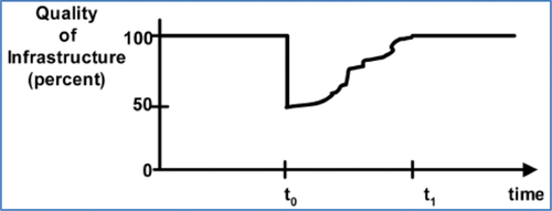
Considering the y-axis as the performance function, ranging from 0% to 100%, the resilience loss is calculated using the following formula:

(1) $RL={\int }_{t_0}^{t_1}\left[100-Q\left(t\right)\right]dt$(1)

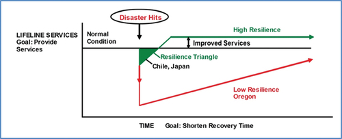
The original resilience triangles approach in infrastructure resilience literature focused on bringing the system back to its state before the disruption. With the increasing intensity and frequency of disasters, experts have acknowledged the importance of ‘building back better’ (BBB), i.e., including elements of enhancements in the recovery process, such that the system is better prepared to manage a similar or worse disruption in the future. The BBB approach was first introduced in 2006 by the UN (Clinton, 2006), and in 2015 was added as a part of the Sendai Framework for disaster risk reduction. Fernandez and Ahmed (2019) have conducted a thorough review of the BBB approach and its evolution over time. The BBB concept has been introduced in the RT approach by multiple researchers, such as Yu et al. (2014), who used the RT approach to compare the seismic resilience of Japan and Oregon and demonstrate Japan’s enhanced resilience by building back better (Figure 2).

Figure 2. Seismic resilience triangle assessment comparing Oregon and Japan’s resilience (Yu et al., 2014).

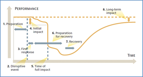
Future detailed applications of the RT approach in supply chains present the non-linear trends in the changes in the performance function as a result of disruption and the long-term impacts of the disruption on the system (Figure 3) (Sheffi & Rice, 2005).

Figure 3. Resilience loss triangle for supply chain (Sheffi & Rice, 2005).

Quantification efforts for resilience in the infrastructure discipline include research in freight and transit systems, with the application of the RT approach in traffic recovery assessments (Tang & Heinimann, 2018), public transit resilience evaluation (Mudigonda et al., 2019), and freight resilience measures (Adams et al., 2012). These efforts to quantify resilience losses can be instrumental in presenting a business case for resilience initiatives to decision-makers by demonstrating, visually as a resilience triangle, how the application of a resilience initiative can reduce the impacts and consequences of a disruption.

While the existing resilience triangle approach presents a cross-sectional view of resilience loss at a given point of time for a specific event, understanding the longitudinal effects of resilience investments in the reduction of future resilience triangles is and will continue to be valuable. This is especially true given the growing need for adaptability and flexibility in systems to ensure improved future responses in the face of evolving uncertainties. There is a gap in the literature of an approach that examines the long-term effects of resilience strategies on the long-term resilience loss of a system.

3. Modified Resilience Triangles (MRT) approach

This paper bridges the existing gap by developing a Modified Resilience Triangles (MRT) approach, which builds on existing resilience triangle approaches and adds modifications that can allow for the long-term benefits of building adaptive resilience to be assessed in systems facing uncertainty.

Three specific aspects of adaptive resilience are reflected in the MRT approach:

1. Long-term RT assessment: In order to use the MRT approach to assess the benefits of resilience strategies, the benefits need to be assessed over the full life of the system, or at least over the life cycle of the resilience strategy being evaluated, as opposed to the current applications of the RT approach which are generally applied at a single-event level (Adams et al., 2012; Mudigonda et al., 2019; Tang & Heinimann, 2018). Long-term assessments will incentivize adaptive resilience investments that foster continuous and reflective learning, as the benefits of such efforts can be quantified.

2. Context-specific system assessment metric (Y-axis): Bruneau et al. note the need for the y-axis to be context-specific, but the resilience triangle has been most traditionally applied with either system performance or system condition as the y-axis. In a complex system, adaptive resilience investments can target any of the multiple possible performance parameters, and in such cases, the appropriate context-specific measure is needed to assess the benefits of such investment. For example, suppose a resilience strategy is focused on building redundancy in the power supply to a transit system. In that case, this enhancement of the system might not be directly reflected in building back better if the y-axis is transit network functionality recovery can only go to 100%, although the system becomes more resilient after the intervention. In such a case, a more appropriate context-specific y-axis would be a composite score of transit network power functionality, such that adding redundancy increases the composite score, thereby counting the resilience benefit in the quantification process.

3. Building back better: While some recent resilience quantification literature does demonstrate building back better in the resilience triangle figure (Figures 2 and 3) (Sheffi & Rice, 2005; Yu et al., 2014), an immediate upward increase might not always be evident. This is especially true in cases where the y-axis is a performance using a percentage scale, which traditionally only goes up to 100%. This does not necessarily mean that such systems cannot be built back better, but rather that the ‘better’ will not directly relate to regular system performance. Instead, it implies that the system will be ‘better’ able to respond to future disruptions. In such cases, a system’s future RTs can be modeled as a function of time, where after each revision or update cycle of the resilience project, there is a possible reduction in the area of future resilience triangles. It is important to note that being able to assess such building back better efforts is dependent on doing a long-term assessment and using a context-specific metric (the first and second modifications presented in the section). The concept is further illustrated in Figure 4.

Figure 4. Resilience loss changes with different adaptive resilience strategy directions.

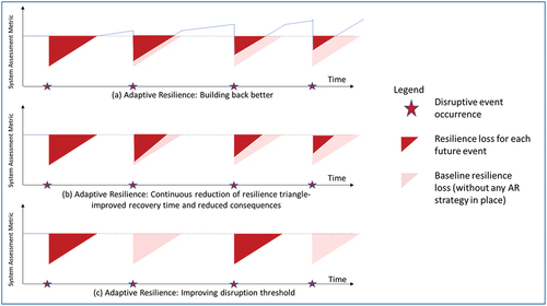
Figure 4 presents the three different ways benefits from adaptive resilience strategies can be accounted for over a long-term time assessment period. Each red triangle demonstrates a simplified version of the resilience triangle during the occurrence of a disruptive event (denoted by a red star on the time axis). As previously discussed in the literature resilience assessment section, the resilience drop, and recovery might follow a curve instead of a straight triangular path. The simplified version in Figure 4 is to demonstrate the different ways adaptations can change the curve.

Responses to the first event in each series occur without any adaptive resilience strategy in place, and all the future RTs are assessed in comparison to the first RT. The first potential adaptive resilience strategy is to build back better (Figure 4(a)), where the same magnitude of loss in functionality on subsequent events would keep the system at a better functional state than the previous, and hence there would be a reduced RT with each new disruption. This building back better occurs at every event, assuming the adaptive resilience strategies include a reflective element which leads to learning from each event and adapting accordingly. Such a representation of improvements in future RTs can be demonstrated if the assessment metric (Y-axis) allows for reflecting continuous improvements over time.

The second way adaptive resilience strategies can enhance long-term system resilience (Figure 4(b)) is by improving the planning and preparation for future absorption, response, and recovery for the system. For investments that do not directly affect system performance, such as workforce training and modular rebuilding process development, the benefits are only evident in the future resilience triangles. A smaller future resilience triangle can demonstrate benefits from such adaptations due to an increased slope of the recovery or a smaller loss in the relevant performance measure on the y-axis. A continuous increase in slope of recovery in future RTs indicates adaptive efforts to enhance future response and recovery efforts, and a continuous reduction in the drop of the y-axis in future RTs reflects adaptive efforts to enhance future absorption of the disruption by the system. The Figure 4(b) indicates both these effects together, but an adaptive resilience strategy can focus on either one or both.

The third pathway an adaptive resilience strategy can take (Figure 4(c)) could be focused on mitigative measures, or measures that reduce the possibility of disruption in the system even with the occurrence of a potentially disruptive event. The common form of such adaptations is raising roadways and increasing the factors of safety in design manuals, such that the threshold for system disruption is increased for any given phenomenon. For example, increasing the bridge height from a 50-yr return period flood level to a 100-yr return period flood level will increase the threshold which the bridge is designed to sustain, therefore potentially reducing the occurrence of resilience triangles in the future. This approach can also be applied to strategies that focus on mitigation, thereby changing the probabilities of occurrence of future disruptions.

A critical aspect of the MRT assessment approach is focused on handling future uncertainty. Climate change is a key factor affecting the occurrence of future RTs in the presented case studies and must be considered when using the MRT approach to assess adaptive resilience investments against natural disasters in infrastructure systems. This, along with other factors of complex infrastructure systems such as urbanization trends, population increase, and economic changes, increase the uncertainty surrounding future resilience loss estimation. The MRT assessment approach uses scenarios for factors with uncertainty where multiple plausible scenarios are identified, for example, using the different RCPs for plausible future scenarios. The assessment approach also uses probabilistic distributions for factors where such data are available, for example, climate models that provide a probabilistic estimate of future precipitation. Finally, it accounts for factors where a general trend exists, such as the time value of money, and sensitivity analysis can be performed to see if there are changes in the results with possible changes in such factors.

4. Assessment methodology

The MRT assessment approach can be segmented into four sections. The first three sections focus on different aspects of input information needed to conduct the assessment, while the fourth segment focuses on the assessment outputs and how to interpret them.

The first section focuses on the system characteristics. The MRT tool provides flexibility in its application where the infrastructure system is not only just the physical asset but the overall socio-technical system involving the complex aspects of the users, organizations, and institutions managing the assets, along with the physical infrastructure asset.

The second section focuses on the disruption characteristics. MRT assessment uses a specific disruption as the base to assess the impacts, or the reduced impacts of such disruption on the system in light of the resilience strategies in place. The disruption characteristics required for the assessment are based on the level of uncertainty associated with the disruption. Scenarios need to be included if the disruption falls under a level of uncertainty where there could be multiple distinctive scenarios that will majorly alter the results, which is the case for the most part while dealing with natural disasters where climate change patterns fall under these uncertainty levels. In such cases, an assessment is performed for each plausible future scenario.

Having identified the scenarios, the assessment of resilience loss over the time period of the assessment is considered for each scenario. Within each scenario, probabilistic estimates of future occurrences of the disruption are used to simulate random events using generalized extreme value distribution or generalized Pietro distributions. A parameter associated with the disruption, which beyond a certain threshold could indicate the occurrence of a disruptive event, is modelled over the time period of the assessment. The last aspect of the disruption characteristics is the event threshold for the baseline case. The threshold might change with the application of different resilience strategies, but for comparison, a threshold as per current standards and assuming a do-nothing or build back to the pre-disruption level’ approach is identified under this section.

The third section inputs requirements of the adaptive resilience strategies. This is where the change in the resilience triangles due to implementing resilience strategies is accounted for. This includes identifying the type of impact the strategy could have on the future RTs, which can be identified from Figure 4. Having identified the type of enhancements that the resilience strategy brings, the next step is to estimate the extent of reduction in the resilience loss in the future. If a strategy is focused on continuous improvement over the time period of the assessment, resilience loss as a function of time is to be identified. If a strategy affects the event occurrence threshold over the assessment time period, then event thresholds as a function of time are to be identified for each such strategy.

The final section of the assessment approach is the output or the results element, where the expected resilience loss for each year of the time period of the assessment is calculated, along with the net present value of the expected resilience loss under the baseline case and with each adaptive resilience strategy implemented. This is calculated for each future scenario, and an overall NPV of resilience loss is estimated based on information on the probabilities associated with the different scenarios.

The step-by-step process of MRT assessment is presented below:

1. Establish the resilience strategies being compared. Let us consider there are no strategies, and one do-nothing strategy to be used as a baseline.

(2) $ResilienceStrategy\left(i\right)=R{S}_i,$(2)

$wherei=\left\{0,1,2,\dots n\right\}$ and baseline strategy occurs at i = 0.

1. Establish the context-specific performance measure (PM) to be used to assess resilience loss in the event of a disruption.

2. Establish the time period of the assessment.

(3) $Time\left(j\right)=T_j,wherej=\left\{1,2,3,\dots \dots .LC\right\}$(3)

where LC = established time period of the assessment. $j$= j^th year in the assessment time frame, where the time frame ranges from $T_1$ to $T_{LC}$.

1. For each resilience strategy ($R{S}_i$), calculate the resilience loss in the system considering a disruption event occurrence at year $T_1$ (the first year in consideration of the assessment’s time period), with the considered strategy in application on the system. Use the resilience triangle approach to calculate the performance metric loss ($R{L}_i$), using the following formula:

(4) $R{L}_i={\int }_{t=1}^m\left(Q_N-Q_i\left(t\right)\right)dt$(4)

Where $R{L}_i=$ Resilience loss in the event of a disruption with resilience strategy i. $Q_i\left(t\right)$ = Performance Metric Function under the resilience strategy i, as a function of time t, where t is the time unit used to assess impacts of each event. Time value t varies from 1 to m, where m is the total time impacted by a single event on the system. The unit of t could range from hours to months – smaller than the unit of T. Q_N = Performance metric Function in the normal state (without any disruption).

1. If any of the strategies impact the resilience triangle of future years, input the resilience loss as a function of time (T). Use the function in equation 3(3) $Time\left(j\right)=T_j,wherej=\left\{1,2,3,\dots \dots .LC\right\}$(3) to calculate the potential resilience loss with each strategy applied, for each year in the future (RL_i,T).

(5) $R{L}_{i,T}=f\left(R{L}_i,T\right)$(5)

1. Identify if there is a factor of low uncertainty that affects the system but is not related to the disruption (population increase, time value of money, and system expansion over time). Use discount rate to account for this uncertainty and create a vector of the factor over time using the current factor value and identified discount rate (DR_T), which is a function of T. If there is no such factor, use a unit value for DR_T .

2. Identify the level of uncertainty related to the future occurrence of a disruptive event. If the uncertainty is high, a scenario-based assessment is needed. In this case, identify and create a list of possible scenarios.

(6) $Scenario=k=\{1,2,\dots .q)$(6)

where q is the number of total plausible scenarios under assessment.

1. Identify a parameter related to the disruption, which can be used to identify the occurrence of a disruptive event by using a threshold on the parameter. For example, if parameter = wind speed, wind speed greater than a pre-defined threshold, indicates occurrence of a hurricane of the category corresponding to the threshold.

2. For each future scenario, use generalized extreme value distribution to generate appropriately randomized values of disruption parameters over the time period of the assessment. The GEV parameters could be time (T) dependent. If the data is available, use time-variable GEV parameters to generate appropriate randomized parameter values for each year. If the data is not available, assume that the GEV parameters are stationary with respect to time. The assumption loses its validity as the time period of assessment increases. Create (r) such simulations, where r is dependent on the computing capacity of the platform where the assessment is being conducted. In applying the approach in this paper, r = 1000, i.e., we ran the simulation 1000 times for each scenario over time period of the assessment.

3. Identify the threshold for the disruption event occurrence with each resilience strategy $(T{h}_i)$. The thresholds could be a function of time if the strategy affects the threshold of event occurrence ($T{h}_i\left(T\right))$

4. Use the thresholds identified in step 9 on the randomized disruption parameter estimates calculated in step 8, to estimate the occurrence of the disruptive event over the time period of the assessment for r simulations. This will create a matrix with dimensions (LC X r), where for each simulation of a time frame of LC years, the event occurrence (OC) value will be 0 or 1, based on whether the corresponding parameter value is smaller or larger than the threshold.

5. Calculate the expected value of resilience loss for each strategy under each scenario by the following formula:

(7) $ER{L}_{ik}\left(T\right)=\frac{1}{r}\times {\sum }_{Sm=1}^{r}O{C}_{i,Sm,k}\times R{L}_i\left(T\right)\times D{R}_T$(7)

Where $ER{L}_{ik}\left(T\right)$ is the expected value of the resilience loss under scenario k, with strategy i in place, for the year T.

$O{C}_{i,Sm,k}$ = {0,1}, based on the value of the disruption parameter generated by the GEV estimates of the kth scenario and threshold Th_i, for the Sm^th simulation. If the value of the parameter for the Sm^th simulation obtained in step 10 is greater than Th_i, OC_i,Sm,k is 1, or else it is 0.

1. Calculate the Net Present Value of the expected resilience loss (for strategy i, under scenario k) across the time period of the assessment, using the following formula:

(8) $E\left(R{L}_{ik}\right)=NPV\left[ER{L}_{ik}\left(T\right)\right]{|}_{T=1}^{T=LC}$(8)

1. If a probability distribution of future occurrence of the different scenarios under consideration is available, the overall expected resilience loss under each strategy can be calculated using the following formula:

(9) $E\left(R{L}_i\right)={\sum }_{k=1}^q{P}_k\times E\left(R{L}_{ik}\right)$(9)

Where, P_k is the probability of occurrence associated with each future scenario. If a distribution is not available, the overall expected resilience loss can be calculated by considering each future scenario equally likely – akin to applying a uniform distribution.

The $E\left(R{L}_i\right)$ for each strategy can be compared with the do-nothing case (baseline), and with the other strategies to determine which one causes the lowest resilience loss to the system and is therefore the best alternative under the considered uncertainties.

5. MRT approach demonstration – case studies

The MRT approach presented in this paper is applied to three different case studies to demonstrate multiple application possibilities of the assessment methodology. Different resilience strategies that support adaptation in each of the three ways presented in Figure 4 are evaluated with the three case studies. The case study subjects capture the different scales of infrastructure systems, with a case study each on a city scale, a transit network scale, and on the scale of a single physical asset (a bridge). The maturity of the adaptive resilience strategies for each of the case studies also varies. For the first case study, the strategy under assessment has already been applied, and adaptive learning from the first applications has been formally identified. A plan has been established for the second case study, but the resilience strategy has not yet been put to the test. In the last case study, the assessment approach is being used to assess multiple possible resilience strategies in order to identify the best approach to plan for in an exploratory setting. With these differences in maturity in the case studies, a good range of possible applications of the MRT assessment approach can be demonstrated.

The first case study focuses on the City of New Orleans and its response to hurricanes that require the city’s evacuation, and the City Assisted Evacuation Plan (CAEP) is the resilience strategy under assessment. The second case study examines the New Jersey Transit Network, where the resilience strategy under assessment is the TransitGrid project, focused on strengthening the resilience of the power distribution of the transit network under future hurricane risks. The third case study focuses on the Tex-Wash Bridge in California, where bridge collapse due to flooding is studied as the disruptive event. The potential adaptive resilience strategies to be compared in this case study are derived from the literature expanding the CalAdapt project conducted by Caltrans, which provides recommendations on different flood management practices for roadway infrastructure such as bridges. In terms of maturity of the adaptive resilience strategies, CAEP in the first case study has been applied once during hurricane Gustav, and further improvements from the lessons learned from the first application have been put into formal documentation for future application. The TransitGrid project in the second case study emerged as a part of the resilience efforts in New Jersey post Sandy. The project has been funded, and the implementation is in progress as of 2021, but the application of the system during a hurricane is not yet tested. In the last case study, the maturity of the resilience strategies application is the most nascent, where multiple possible strategies are being assessed for a comparative analysis that can be used to select the best strategy to be planned and implemented in the future.

5.1. New Orleans hurricane evacuation – city assisted evacuation plan

In August 2005, Hurricane Katrina, which was a category five hurricanes at its peak, made landfall in Louisiana as a category three hurricanes and had catastrophic impacts, including over 1000 fatalities in Louisiana alone. Safe evacuation was a challenge to the city officials. While Louisiana evacuated almost 1.5 million people before Katrina made landfall, almost 150,000 people did not or could not evacuate (Zimmermann, 2015). Many of those who did not evacuate, did so due to lack of resources. The plans made during the event’s unfolding to evacuate those without personal vehicles were cancelled due to roads being clogged by those self-evacuating. Lack of foresight in planning for the vulnerable populations caused many to die. In the City of New Orleans, almost 30% of the population does not own a car, and more than 25% of the population lives below the poverty line (Wade, 2017). With the lessons learned from Katrina, the City of New Orleans developed an improved emergency management plan, which includes a formal evacuation plan – City Assisted Evacuation Plan (CAEP), for those who cannot evacuate by themselves (Kiefer et al., 2009).

The plan was applied during Hurricane Gustav in 2008, where approximately 18,000 people were evacuated using CAEP. While mostly considered successful, gaps were identified in its application, and further assessments and studies were conducted to improve the plan for a better future implementation (Kiefer et al., 2009; Schrilla, 2019). The development, implementation, and reflective learning in the planning of CAEP is reflective of adaptive resilience being practiced by the city. The use of diverse stakeholders such as NGOs, federal and state government, private agencies, under the guidance of the Office of Homeland Security and Emergency Management, and formalized reflective learning demonstrated after the first application present some of the critical attributes of adaptive resilience from the city.

5.1.1. MRT approach assessment

This case study evaluates the resilience benefits of the implementation of CAEP in the City of New Orleans. The infrastructure system under consideration is the City of New Orleans, which comprises the users, public transit infrastructure, the shelter infrastructure, among the other elements of the city affected, or being utilized for a system-level response to disruptions. The disruption considered in the study is a hurricane category three and above – a disruption that would demand a mandatory evacuation by the city. A 50-year time period is considered for assessment (LC =50). The assessment will compare the following four cases of resilience strategies (RS_i):

1. If CAEP did not exist (RS₀)

2. If CAEP is applied during future evacuations just as it was applied during hurricane Gustav (no future improvements) (RS₁)

3. If CAEP is applied during future evacuations with the improvements identified from Hurricane Gustav Lessons (assuming complete application of the lessons learned from Gustav; RS₂; Kiefer et al., 2009; Schrilla, 2019)

4. If CAEP is applied with continuous improvements identified and implemented every ten years (assuming reflective learning and improvements will continue on a formal basis) (RS_{3 –} RS_n)

The first case can be used to assess the relative benefits of cases 2–4. The 3^rd and 4^th cases are forward-looking cases, which can be used to estimate the future benefits of investing in improving the program. Such information could be helpful for decision makers for project prioritization.

The resilience triangle for each case is estimated using historical data and future assumptions based on literature review and expert input. Given that CAEP is developed to provide better evacuation response for those who cannot evacuate by themselves, the context-specific performance measure to assess the resilience benefits provided by the program needs to reflect the same. The context-specific assessment metric here is a multi-criteria metric to assess the availability of essential services – ESAI (Essential Services Availability Index). ESAI can be considered an equivalent metric of quality of life, but for disaster evacuees (Puskorius, 2015).

ESAI for any fraction of the population would be a factor of the satisfaction level of that population with the essential services availability. During an evacuation process, people can be categorized to be in one of the three situations: 1) self-evacuate to friends/family/hotel, 2) use CAEP for evacuation, 3) do not evacuate. Based on previous information about shelters, the 2^nd situation can be sub-categorized into two situations: 2(a) – CAEP with sufficient capacity, 2(b) – CAEP with reduced capacity. This categorization is based on the fact that for Hurricane Gustav, the CAEP shelters and transport facilities ran out of capacity mid-way during the evacuation effort (Brodie et al., 2006; Fetters, 2018). This will change the availability of essential services to those using CAEP.

The value of ESAI for any given day during the event time frame could be calculated using the following formula.

(10) $Q\left(t\right)=ESA{I}_t={\sum }_{j=1}^m(P_j\times S_j{)}_t$(10)

where,

• t = time (in days) Time ranging from t₀-t_1, where t₀ is the time (days) before the evacuation order is put in place, and t₁ is the time by which recovery of the event is complete

• P_j = percentage population in the j_th availability situations

• S_j = satisfaction factor (weighting factor) of the essential services availability in the j_th scenario.

• m = maximum number of different types of possible essential service availability situations (here, m = 5: 1- all services met (normal state), 2- shelter at friends/family, 3- shelter with CAEP with full capacity, 4- shelter with CAEP with reduced capacity, 5-stuck in the hurricane with no services)

Jordan (2015) provides a hierarchy of needs of disaster survivors, which can be used as the essential services needed for the evacuees. The weights associated with each need are assumed to follow a centroid weight distribution, with the highest weight given to the lower order needs of food, water, and shelter and subsequently lower weights to the higher-order needs in the hierarchy. The weight distribution and the essential needs being used for assessment were validated via expert interviews of those involved in Hurricane Katrina and Hurricane Gustav’s evacuation efforts. The interviews were also used to identify which of these essential needs were fulfilled in each of the four situations. The percentage of the population in each situation was estimated based on Hurricane Katrina and Hurricane Gustav data.

Calculation of the resilience loss in each case (RL_i) uses the data from Hurricane Gustav and Katrina’s evacuation efforts to estimate the percentage of the target population in each situation for each case. As per Hurricane Gustav CAEP’s use survey (Kiefer et al., 2009), about 40% of those who registered for CAEP used other means to evacuate, about 42% of those registered used CAEP, and about 18% did not evacuate. The target population is the population that cannot evacuate by themselves and would need CAEP or other support to evacuate. In the case of RS₀, which is the case without CAEP, it is assumed that a total of 60% of the target population did not evacuate. This could be assumed as those who could have used CAEP and could not find any other way to evacuate (42%) will not be able to evacuate, along with those who choose not to leave (18%). In the case of RS₁, the original data from CAEP’s application is used. In the case of RS₂, RS₃, and RS_n, it is assumed that the improvements are in the satisfaction factor of the essential services provided by CAEP, and efforts to spread awareness of the program to nudge the 18% people who would otherwise choose not to evacuate. RS_n is estimated assuming the best case of application of CAEP, in which the shelters are at the same satisfaction level as evacuation to friends/family, and all of the 18% population is successfully nudged to use the program to evacuate. RS_n is used to calculate the linear trend of improvements over time in the CAEP program until the best possible application is achieved, in order to explore the potential benefits of the fourth case of continuous improvement in the program.

Due to climate change, the future occurrence of hurricanes cannot be predicted with a reasonable level of confidence. Sea Level Rise has a direct correlation with the frequency and intensity of hurricanes (Marsooli et al., 2019; Wdowinski et al., 2016). Hence, three future SLR scenarios are considered for assessment. The probability estimates of the three scenarios are based on Intergovernmental Panel on Climate Change (IPCC) estimates (Field et al., 2014). For each SLR scenario, a Generalized Extreme Value function for hurricane wind speed is used to generate 1000 simulations for maximum wind speed over the time period of assessment. The GEV parameters based on historical data are obtained from the existing literature, and change in parameters under different SLR scenarios is estimated from the change in return periods of events for each SLR as identified by IPCC and other literature (IPCC, 2019; Keim et al., 2007). The wind speed threshold for hurricane category 3+ is obtained from the Saffir-Simpson Hurricane Wind Scale (NOAA, n.d.).

Table 1 summarizes all the data inputs for the MRT assessment and Table 2 provides the GEV parameters for the different SLR scenarios.

Table 1. MRT assessment steps- input.

1	Resilience Strategy(i)	CAEP | (RS0 … … RSn)
2	Context-specific performance measure (Q)	Essential Services Availability Index (ESAI)
3	Time period of assessment	50 years
4	RL(i) calculation	[See the results section]
5	RL(i,T)	RL4 as a function of time – linear improvement every 10 years from RL1 to RLn over the LC
6	f(T)	Population (future projections based on census data)
7	Scenarios (k)	K = {1,2,3}: SLR – Low, SLR – low-intermediate, SLR – Intermediate-High (based on IPCC)
8	Disruption Parameter	Hurricane Wind Speed
9	GEV parameters	[See, Table 2]
10	Disruption threshold	96 knots (Hurricane category 3 wind speed)
11–14	Results Calculation	[See the results section]

Table 2. GEV parameters for the different SLR scenarios.

	GEV parameters
Scenario	Location (µ)	Scale (σ)	Shape (ξ)
Baseline- Low SLR	64	36	−0.37
Low-Int SLR	66.47	36	−0.37
Int-High SLR	69.09	36	−0.37

5.1.2. Results

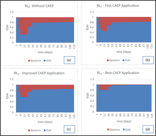
Figure 5 presents the resilience triangles for the four different cases of the resilience strategy application. The red area indicates the resilience loss during the time of the disruption event. The x-axis ranges from 1 to 113, based on Hurricane Katrina’s duration of evacuation and recovery. It is evident that with better application of CAEP, the resilience triangle is continuously reducing, indicating the benefits of the resilience strategy.

Figure 5. Resilience triangle for different RL cases- CAEP.

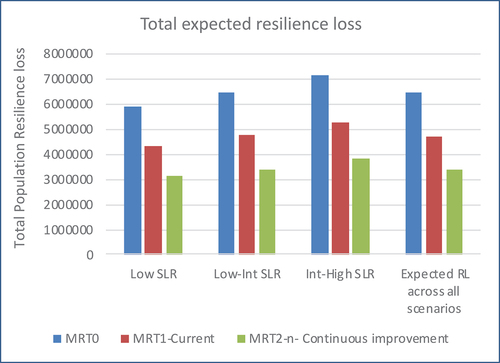
The point values of resilience loss (ESAI units) are used along with disruption uncertainty to estimate the resilience loss over the time period of the assessment. If an event occurs in a given year, for each case, the total area under the resilience triangle, multiplied by the total target population for that year is considered the resilience loss for that year. Expected resilience loss over the 1000 simulations is presented for the time period of the system for each scenario in Figure 6(a-c). The y-axis is the resilience loss area for the given case for the year, multiplied by the overall target population (Population Resilience Loss). The figures show the resilience loss for the RS₀: no CAEP case, RS₁: Current CAEP application, and RS_2-n: CAEP application with continuous improvement. It also indicates that without CAEP, with an increasing population, the resilience loss is increasing over time. While for the initial years in the life cycle, RL₁ and RL_2-n show similar results, with continuous improvements, the overall resilience loss of the RL_2-n is decreasing over time. The expected value of the resilience loss over the assessment’s time period is presented in Figure 7, along with an overall expected resilience loss estimate based on probabilities associated with each SLR scenario. It indicates a lower resilience loss with CAEP in application compared to the case without it and further reduction in resilience loss with continuous improvements in the system. While the results are intuitive, the assessment provides quantitative values to compare the benefits of implementing any given resilience strategy.

Figure 6. Expected resilience loss for each year in the assessment timeframe for each SLR scenario – CAEP.

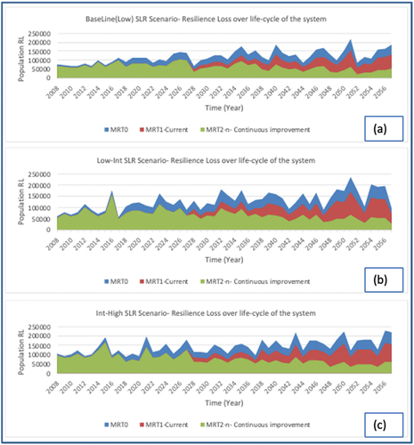
Figure 7. Total expected resilience loss over the time period of the assessment for each SLR scenario, and the expected RL across all scenarios.

5.2. NJ transit power outage – NJ transitgrid

Hurricane Sandy in 2012 exposed the vulnerabilities of the transit systems in New York and New Jersey. The centralized power system breakdown during Sandy significantly disrupted the NJ Transit functioning (Comes & Van de Walle, 2014). NJ Transitgrid project is developed to build resilience against this identified vulnerability of the NJ Transit System. Transitgrid is one of the many projects being developed as part of the Resilience Program by NJ Transit, which came into action after Hurricane Sandy (NJ TRANSITGRID n.d.). Under the Transitgrid project, NJ Transit plans to construct an electrical microgrid system capable of supplying power to some key parts of the network during future storms, which could cause the centralized power system to fail. Transitgrid project promotes adaptive resilience by building in modularity and redundancy in the system, as it provides multiple sources of power to the network, thereby increasing its chances of sustaining network functionality when one of the power sources fails. The project is funded by a grant awarded by Federal Transit Administration (FTA) through its emergency relief program in response to Superstorm Sandy (NJ TRANSITGRID n.d.). The project has not yet been implemented and tested with any disruption. Hence, the estimates of its functionality in case of disruption are assessed by applying the project on hurricane Sandy’s timeline and assuming that the system will function as planned. The assessment could be improved in the future as the project is put to real test by a disruption, and the model can be calibrated based on observed data.

5.2.1. MRT approach assessment

This section evaluates the benefits of implementing Transitgrid in improving the resilience of the NJ Transit network. The infrastructure system under consideration is the NJ Transit network of rail lines. The disruption considered in the study is a hurricane category 3 (Sandy made landfall as a category three hurricane in NJ). A 50-year time period is considered for assessment (LC =50). The assessment compares three cases of resilience strategies (RS_i):

1. If Transitgrid is not put in place (RS₀)

2. If Transitgrid is applied during future disruptions as per the current plans (RS₁)

3. If Transitgrid is applied during future disruptions with an increase in its network coverage after ten years (potential project expansion) (RS₂)

As the project has not yet been implemented, unlike CAEP, where the first implementation and lessons have already been established, the improvements for Transitgrid are only projected one step ahead – with an assessment of the impacts of a possible expansion at year 10.

The context-specific performance metric here is a score of transit network functionality, which is a score accounting for the power redundancy of the system. The following formula can represent the Transit Functionality Score:

(11) $TFS={\sum }_{i=0}^{i=n}i\times P(R{M}_i)$(11)

• n = maximum number of power sources available to a given mile of transit (in this case, i ={0,1,2} – max two sources of power)

• P(RM_i) = Percentage of rail miles with i number of power sources

• Without TransitGrid, all of the rail miles are served with only one power source in normal conditions (centralized power system), i.e., i ={0,1}

• With TransitGrid (as of current plans), a small, selected percentage of rail miles have access to two power sources during regular times, and when the centralized power is cut off, the percentage of rail miles has one source of power (TransitGrid)

• Enhancements on TransitGrid plans could expand on the coverage of the program for a higher percentage of rail miles

Table 3 presents the key inputs on the MRT assessment steps for this case study.

Table 3. MRT assessment steps: data inputs for transitgrid.

1	Resilience Strategy(i)	TransitGrid | (RS0, RS1, RS2)
2	Context-specific performance measure (Q)	Transit Functionality Score (TFI)
3	Time period of assessment	50 years
4	RL(i) calculation	[see the results section]
5	RL(i,T)	RL2 as a function of time – first potential improvement at year 10, constant thereafter
6	f(T)	Rail miles (expansion of rail miles over time- NJ Transit data)
7	Scenarios (k)	K = {1,2,3}: SLR – Low, SLR – low-intermediate, SLR – Intermediate-High (based on IPCC)
8	Disruption Parameter	Hurricane Wind Speed
9	GEV parameters	[see, Table 4]
10	Disruption threshold	96 knots (Hurricane category 3 wind speed)
11–13	Results Calculation	[see the results section]

Disruption uncertainty is modeled similarly to the CAEP case study, with the GEV parameters of hurricane wind speeds estimated for the NJ region. Table 4 presents the GEV parameter estimates for this case study.

Table 4. GEV parameters for NJ hurricane wind speeds.

	GEV parameters
Scenario	Location (µ)	Scale (σ)	Shape (ξ)
Baseline- Low SLR	77.2	10.6	−0.0544
Low-Int SLR	79.49	10.6	−0.0544
Int-High SLR	83.25	10.6	−0.0544

5.2.2. Results

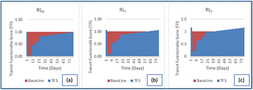
Figure 8 presents the resilience triangles for the three cases of the resilience strategy application. The red area indicates the resilience loss during the time of the event. The x-axis ranges from 1 to 73, based on Superstorm Sandy’s transit network disruption and recovery duration. It is evident that with better application of Transitgrid, the resilience triangle is reduced, indicating the benefits of the resilience strategy. The RL₁ and RL₂ triangles also indicate an immediate improvement in the level of TFI, indicating building back better. A value higher than one corresponds to the fraction of the network with more than one power source in normal conditions.

Figure 8. Resilience loss for different cases of transitgrid application.

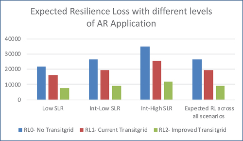
The point values of resilience loss are used along with disruption uncertainty to estimate the resilience loss over the time period of the assessment. If an event occurs in a given year, for each case, the total area of the resilience triangle is considered the resilience loss for that year. Expected resilience loss over the 1000 simulations is presented for the time period of the assessment for each scenario in Figure 9. The y-axis is the resilience loss value, multiplied by the total rail miles of the network for the given year for the given case (miles of network with reduced functionality score). The figures show the resilience loss for the RS₀- no Transitgrid case, RS₁- Current planned Transitgrid application, and RS₂- Potential expansion of Transitgrid by 10% at year 10. The expected value of the resilience loss over the assessment’s time period is presented in Figure 10, along with an overall expected resilience loss estimate based on probabilities associated with each SLR scenario. The figure indicates a lower resilience loss with Transitgrid in application compared to the case without it, and further reduction in resilience loss with improvement in the project. These results are consistent with the CAEP case study, only differing in the lack of a continuous improvement case, with respect to which the CAEP case study is currently at a higher maturity level.

Figure 9. Expected resilience loss for each year in the assessment timeframe for each SLR scenario -Transitgrid.

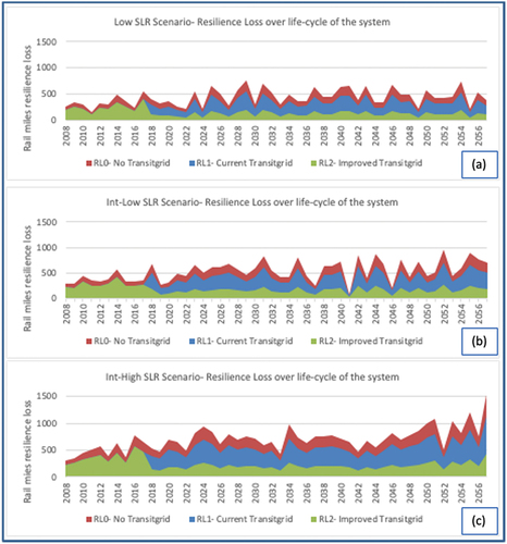
Figure 10. Total expected resilience loss over the timeframe of the assessment for each SLR scenario, and the expected RL across all scenarios – Transitgrid.

5.3. Tex-Wash Bridge closure, California – DAP

On July 19^th, 2015, extreme precipitation of over 6 inches in a day caused flash flooding in Riverside County in California, which caused the Tex-Wash Bridge to collapse. The bridge was rebuilt back to previous design standards with almost an $8 million rebuild cost (Tabbakhha et al., 2016). With uncertainty in future precipitation projections and increasing frequency and intensity of extreme events, building back to the previous design standards might not be the optimal decision in the long term. In this case study, we compare different possible resilience strategies that can enhance the bridge’s resilience against such events in the future. While currently no such plan exists for this specific bridge, the data of the disruption impact can be used for a demonstrative example for bridge flood management, or any asset-specific resilience effort for transportation agencies.

This assessment compares static plans of transportation flood management with a Dynamic Adaptive Plan for the same. With increasing uncertainty associated with climate change, dynamic adaptive plans are more aligned with the adaptive resilience approach, allowing for flexibility in future actions, and preventing roadblocks while reducing significant upfront investments. Dynamic Adaptive Planning is one of the four established approaches for decision-making under deep uncertainty, where the plans are designed to evolve with evolving nature of variables uncertain at the time of plan development. Under the 2010–2011 FHWA Climate Change Vulnerability Assessment Pilot program, the metropolitan planning organization (MPO) of San Francisco conducted a study – Adapting to Rising Tides (ART) (Kline et al., 2011). The study assessed the impacts of SLR and coastal flooding and provided recommendations on possible actions based on mid-century (~year 2050) and end-century (~year 2099) predictions of future disruptions. Wall et al. (2015) built on the study and demonstrated a Dynamic Adaptive Plan (DAP) building on the actions identified in the ART study. Singh et al. (2020) conducted a quantitative assessment of the DAP approach vs. the two static approaches to capture the value of flexibility in transportation resilience planning. In this paper, we use the approaches presented by Wall et al. (2015) and Singh et al. (2020) to generate static mid-century (~ year 2050) and end-century (~ year 2099) plans, and a dynamic adaptive plan for the bridge under consideration and compare their resilience benefits over the time period of the assessment. Using a DAP approach reflects the agency’s capabilities in roadmapping, and the successful implementation of DAP is only possible with an organic finance structure in the system to allow for planning for flexibility in investment in the future. These capabilities reflect the adaptive resilience maturity of an agency. With a DAP, the agency has the capability to adapt to the changing conditions by monitoring the near-term projections (~5 years into the future) and make changes to the system depending on the direction the system is headed. This ensures that the DAP is not developed to cater to a specific projection model, but rather has specific actions pre-defined that can be taken at any time in the future, identified by the monitoring triggers. The timing of these triggers will depend on the scenario that unfolds in the future, but the DAP approach will be applicable in most of such scenarios.

5.3.1. MRT approach assessment

This section compares the benefits of implementing different resilience strategies in improving the resilience of a bridge. The infrastructure system under consideration is the Tex-Wash Bridge. The disruption considered in the study is a bridge collapse event which could occur at different extreme precipitation levels based on the flood protection level of the bridge. A 90-year time period is considered for assessment (LC =90) based on future projection data availability. The assessment compares the following four cases of resilience strategies (RS_i):

1. The bridge is built back to previous standards (current state) (RS₀)

1. Improvements are made based on current mid-century projections from a selected projection model (RS₁)

2. Improvements are made based on current end-century projections from a selected projection model (RS₂)

3. Dynamic improvements are made over the time period of the assessment based on emerging data over time (DAP) (RS₃)

The context-specific performance metric here is the economic benefit provided by the bridge (EBB), which is lost when the bridge is closed:

(12) $EBB\left(\mathrm{\$}\right)=C_{pv}\times AADT+C_T\times AADTT$(12)

• ${\mathrm{C}}_{\mathrm{p}\mathrm{v}}$= Detour cost of passenger vehicles

• ${\mathrm{C}}_{\mathrm{T}}$ = Detour cost of trucks

Any of the four adaptation options do not reduce the EBB loss if the bridge collapses but reduce the potential occurrence of the collapse event by improving the threshold – RT stays the same for any future disruption, but the frequency of disruption is potentially be reduced (Figure 4(c)).

Disruption uncertainty is modeled based on projected future precipitation data developed by Cal-Adapt (Cal-Adapt, 2021), whose database of downscaled climate change projections was developed by the Geospatial Innovation Facility at the University of California. The future projections are based on different projection models. While the Cal-Adapt research provides 10 different climate model projections, for demonstration purposes, two of the extreme models are considered in this case study. These two models are considered here for assessment as the two possible scenarios with level 3 uncertainty (lack of confidence in which model will unfold in the future). These models, modeling potential future scenarios, emerged from California’s Fourth Climate Change Assessment, 2018 (CA.gov., 2018). The two models considered for this assessment cover the two opposite future scenarios, with a cool/wet future presented by the CNRM-CM5 model and a warm/dry future presented by the HadGEM2-ES model (Pierce et al., 2018). For each of these two models, the data corresponding to RCP 4.5 is used in the assessment. To calculate the total resilience across both scenarios, each scenario is considered equally likely. The future projected data is the maximum annual precipitation intensity (1-day precipitation in inches) for the 5-mile grid on the bridge location directly available from each model scenario. These data are used to calculate the GEV parameters and are also used to calculate the change in GEV parameters over time. This provides a better reflection of climate change over time in accounting for future uncertainty in the assessment. Table 5 presents the key inputs on the MRT assessment steps of this case study.

Table 5. MRT assessment inputs: Tex-Wash Bridge.

1	Resilience Strategy(i)	Bridge Flood Management | (RS0, RS1, RS2, RS3, RS4)
2	Context-specific performance measure (Q)	Economic benefit of the bridge ($)
3	Time period of assessment	90 years
4	RL(i) calculation	[See the results section] All RL(i) have the same value
5	RL(i,T)	-
6	f(T)	Time value of money – discount rate of 5%
7	Scenarios (k)	K = {1,2}: Two future projection models – CNRM-C5 (Cooler/Wetter), and HadGEM2-ES(Warm/Drier)
8	Disruption Parameter	Max daily precipitation
9	GEV parameters	Calculated using projection models
10	Disruption threshold	Variable with each strategy [see, Table 7]
11–13	Results Calculation	[See the results section]

The disruption threshold varies based on the resilience strategy implemented:

1. RS₀: Build back to previous standards- the threshold would be the same value at which the bridge collapsed – 6 inches of rainfall in a day.

1. RS₁: Mid-century static plan – the threshold would be the mid-century estimate of 100-yr return level precipitation estimated by each model at the start of the assessment timeline.

2. RS₂: End-century static plan – the mid-century estimate of 100-yr return level precipitation estimated by each model at the start of the assessment timeline.

3. RS₃: Dynamic adaptive plan – Various potential future action steps are identified and planned, and monitoring systems are set up to identify the trigger point when the pre-defined actions will need to be taken. The evolving design threshold of the bridge is based on triggers identified from the near-term future projection of a 100-yr return level. Every year (in each model scenario), the 100-yr return level is calculated 20 years in the future, and if the value goes beyond the identified trigger, a corresponding adaptation action is applied, thereby increasing the threshold by a set amount.

Table 6 presents the details of the variable thresholds with the triggers used in the DAP process. Table 7 presents the thresholds for the three static plans for each scenario.

Table 6. DAP triggers and improved thresholds.

Trigger	Action	Improved threshold
Trigger 0: 100-yr return level projected 20 years from time (T) is less than 6 inches	No action	6 inches
Trigger 1: 100-yr return level projected 20 years from time (T) is between 6–8 inches	Deck rehab (raising/strengthening)	8 inches
Trigger 2: 100-yr return level projected 20 years from time (T) is between 8–10 inches	Deck replacement	10 inches
Trigger 3: 100-yr return level projected 20 years from time (T) is between 10–12 inches	Deck replacement+ superstructure & substructure rehab	12 inches
Trigger 4: 100-yr return level projected 20 years from time (T) is greater than 12 inches	bridge replacement	14 inches

Table 7. Thresholds for static resilience strategies.

Resilience Strategy	CNRM-CM5 Model	HadGEM2-ES Model
RS0 (Build back same)	6 inches	6 inches
RS1(mid-century plan)	8.23 inches	7.09 inches
RS2(end-century plan)	10.25 inches	8.37 inches

5.3.2. Results

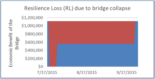
Figure 11 presents the resilience triangle for the case of bridge collapse based on the 2015 event details. The red area indicates the resilience loss during the time of the event, calculated in terms of economic loss of passenger and freight traffic due to detours. The x-axis is a timeline of the event, from July 2015, when the bridge closed, to Sep 2015, when the bridge came back to full functionality. As the resilience strategies under assessment do not change future resilience triangles, but change their frequency of occurrence, only one resilience triangle is needed for the assessment.

Figure 11. Resilience loss triangle for bridge closure\Tex-Wash Bridge.

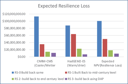
Expected resilience loss over the 1000 simulations is presented for the time period of the assessment for each scenario in Figure 12. The y-axis is the resilience loss value for the given year for the given resilience strategy. The figures indicate reduced resilience loss with each of the resilience strategies compared to the strategy of building back to the same level. It can also be observed that the end-century static plan has smaller resilience loss compared to the mid-century plan, which makes sense as with the increasing frequency of the disruptions as presented by the models, the threshold for the static mid-century plan will not be sufficient over the assessment’s time period. Comparing the end-century static plan with the DAP, the results indicate that the DAP has higher resilience loss for earlier years in the time period than the end-century static plan, which can be understood as DAP gradually increases the system’s threshold to disruption, but the end-century plan starts with a higher threshold. This allows the end-century plan to reduce the potential resilience loss under rare extreme events beyond the estimated DAP thresholds. However, as we move forward in the time period, the resilience loss of the static end-century plan is increasing as the return level is continuously increasing over the time period of the assessment due to climate change. However, the static plan’s threshold is based on previous static information, while the DAP continues to improve its thresholds using the updated information. The expected value of the resilience loss over the system’s life cycle is presented in Figure 13, along with an overall expected resilience loss estimate based on equal probabilities associated with each climate model scenario. The figure also indicates the smallest resilience loss over the assessment’s time period under the DAP resilience strategy. Using this information, along with the fact that upfront capital investment for the 2^nd best strategy (the end-century static plan) will be much higher than that of DAP, it makes more of a business case to use a flexible, evolving strategy that has overall higher benefits, and smaller upfront investment cost.

Figure 12. Expected resilience loss for each year in the assessment timeframe for each SLR scenario -Tex Wash Bridge.

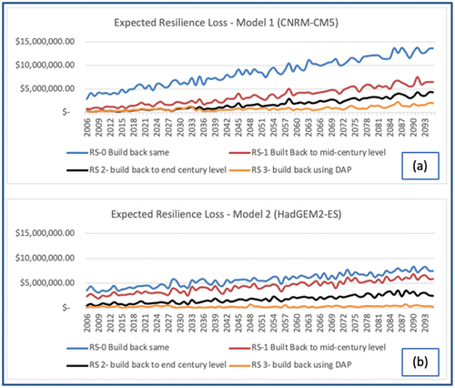
Figure 13. Total expected resilience loss over the time period of the assessment for each SLR scenario, and the expected RL across all scenarios – Tex Wash Bridge.

5.4. Overall results

Results across all the three case studies indicate significant benefits (or reduced resilience loss) of adaptive resilience strategies as compared to the baseline (do-nothing or build back without adaptation). Further, continuous improvements in the adaptive strategies reflect increasing benefits over time, which makes a case for investing in plans and procedures established for reflective learning through one or more lifecycles of the system. Table 8 presents the relative reduction in the expected resilience loss for each case study across all considered scenarios. It indicates that a one-time implementation of AR strategy resulted in an approximately 27% reduction in loss for both the CAEP and TransitGrid case studies with an even higher resilience loss reduction (48% and 66% respectively) under the case where the AR strategies were improved over time. For the Tex-Wash Bridge case study, the AR strategy of DAP presents a 92% expected reduction in loss compared to build-back to the same level scenario.

Table 8. Percentage reduction in expected resilience loss with different AR strategies across all considered scenarios.

CAEP		TransitGrid		Tex-Wash Bridge DAP
-	-	-	-	RL1- Built Back to mid-century level	51%
RL1-Current CAEP	27%	RL1-Current TransitGrid	27%	RL2- build back to end century level	82%
RL2- Continuously Improved CAEP	48%	RL2- Improved TransitGrid	66%	RL3- build back using DAP	92%

These results demonstrate significantly long-term benefits of adaptive resilience strategies, continuous reflective learning, and flexible long-term planning, thereby presenting a strong business case for investment in such adaptive resilience strategies.

6. Conclusion

Quantification of long-term benefits of adaptive resilience strategies is critical in making a stronger business case for long-term planning that incorporates flexibility and agility as key attributes to augment adaptive resilience. Such quantifications can also support project prioritization for practitioners by providing an objective measure of the performance of the projects, as demonstrated by the third case study. Efforts in long-term planning for system resilience with an intentional efforts towards adaptive resilience is key for a holistic resilient system under future uncertainty. Hence an approach that quantifies the long-term benefits of such adaptive resilience strategies is beneficial for decision makers to use for effective project prioritizations. This paper presents an approach for agencies to assess their investments in building resilient infrastructure systems, over a range of scales of infrastructure and type of resilience strategies. The three case studies demonstrate the range of possible applications of the MRT approach, with results indicating a general trend towards higher benefits with more flexible and adaptive strategies in the long term. The approach presented in the paper can be used by public and private agencies in multiple infrastructure sectors such as transportation, power, water, and communication. A flexible approach to evaluate the long-term benefits of building adaptability as a part of enhancing resilience in the system can serve as a helpful tool for practitioners and policymakers to present a business case for long-term adaptive resilience investments.

6.1. Limitations and future work

Some of the limitations in applying the MRT approach in the case studies came from the availability of data. While for the third case study, quality downscaled future projection data was available, from which we were able to estimate the time-variability of future disruption estimates, the lack of similar data for the first two case studies limited our assessment to a smaller timeframe, within which the GEV parameters did not change over time. The confidence in the results of the approach will increase with improved data inputs of future projections. In the first case study, where the resilience strategy is focused on the social infrastructure of the city, the quantification of satisfaction of disaster evacuees in the shelters is based on expert input. As the event under consideration occurred over a decade ago, the input from experts might not be very accurate. Better documentation of future applications of CAEP and immediate surveys of evacuees will help validate the inputs used in the case study. Another limitation of the demonstrated application of the approach is in quantifying the time value of non-monetary assessment metrics. While for the third case study where the metric was monetary, a discount rate could be used to reflect the time value of the metric, for the other two case studies, it was assumed that the value of the non-monetary metrics does not increase (or decrease) over time. Future work to assemble better records of such non-monetary metrics could help in estimating their discount factors.

A general limitation of the application of the approach in the three case studies is the set of assumptions used in the illustration of the approach. While the approach theoretically is designed to be generalizable and scalable, the case studies do not focus on studying the sensitivity of the results to a range of uncertainty factors. The quantification of the resilience loss in each of the case studies can be enhanced in accuracy by improving the data sources. A thorough look into the various parameters defining the resilience in each case study and quantitative analysis if their independence is warranted, while in this study, they are assumed to be independent, backed by either expert input or literature review, both of which are subjective approaches and can be strengthened by a more holistic assessment.

Further work on incorporating the MRT approach in the formal asset valuation and asset management plans of infrastructure agencies will support its application in practice. The MRT approach can also be used in combination with other approaches such as real options analysis to value investments under uncertainty in order to increase the flexibility in the dynamic plans instead of associating fixed time frames with improvements as depicted in this paper. Further, incorporating the MRT approach in benefit-cost assessment approaches at infrastructure agencies could enhance the BCA analysis and support better project prioritization efforts.

Acknowledgments

The authors acknowledge the practitioners and experts from New Orleans who participated in the expert interviews for their input in the MRT application for CAEP case study. Their identifiable information is kept confidential as per the IRB guidelines.

Disclosure statement

The Coalition for Disaster Resilient Infrastructure (CDRI) reviewed the anonymised abstract of the article, but had no role in the peer review process nor the final editorial decision.

Additional information

Funding

This work is supported in parts by the GDOT Research Project - Incorporating Resilience Considerations in Transportation Planning, TSMO and Asset Management (GT RP 20-12), and the Georgia Institute of Technology 2020 Small Bets Seed Grant 2020 Small Bets Grant Award - Black Swan Event Identification and Planning for Urban System Resilience. The Article Publishing Charge (APC) for this article is funded by the Coalition for Disaster Resilient Infrastructure (CDRI).

Notes on contributors

Prerna Singh

Prerna Singh, Ph.D., Transportation Sector Specialist, UNDP, School of Civil and Environmental Engineering, Georgia Institute of Technology, Atlanta, GA, USA. E-mail: [email protected].

Adjo Amekudzi-Kennedy

Adjo-Amekudzi-Kennedy, Associate Chair for Global Engineering Leadership and Entrepreneurship, Frederick L. Olmstead Professor, Georgia Institute of Technology, Atlanta, GA, USA. E-mail: [email protected].

Baabak Ashuri

Baabak Ashuri, Professor, Schools of Building Construction, and Civil & Environmental Engineering, Georgia Institute of Technology, Atlanta, GA, USA. E-mail: [email protected].

Mikhail Chester

Mikhail Chester, Civil, Environmental, and Sustainable Engineering, School of Sustainable Engineering and the Built Environment, Arizona State University, Tempe, AZ, USA. E-mail: [email protected].

Samuel Labi

Samuel Labi, Professor of Civil Engineering, Purdue University, Lyles School of Civil Engineering West Lafayette, IN 47907-2051. Email: [email protected].

Thomas A. Wall

Thomas A Wall, Program Lead, Engineering & Applied Resilience, Decision and Infrastructure Sciences Division., Argonne National Laboratory, USA. E-mail: [email protected].

References

- AASHTO. (2017). Understanding transportation resilience: A 2016-2018 roadmap |.
- Adams, T. M., Bekkem, K. R., & Toledo-Durán, E. J. (2012). Freight resilience measures. Journal of Transportation Engineering, American Society of Civil Engineers, 138(11), 1403–1409. https://ascelibrary.org/doi/abs/10.1061/(ASCE)TE.1943-5436.0000415. doi:10.1061/(ASCE)TE.1943-5436.0000415.
- ASCE. (2013). Policy statement 518- Unified definitions for critical infrastructure resilience (ASCE).
- Bosello, F., & Chen, C. (2011). Adapting and mitigating to climate change: Balancing the choice under uncertainty. SSRN Electronic Journal. https://doi.org/10.2139/ssrn.1737614. FEEM Working Paper No. 159.2010.
- Brodie, M., Weltzien, E., Altman, D., Blendon, R. J., & Benson, J. M. (2006). Experiences of hurricane Katrina evacuees in Houston shelters: Implications for future planning. American Journal of Public Health, 96(8), 1402–1408. https://doi.org/10.2105/AJPH.2005.084475
- Bruneau, M., Chang, S. E., Eguchi, R. T., Lee, G. C., O'Rourke, T. D., Reinhorn, A. M.,& Von Winterfeldt, D. (2003). A framework to quantitatively assess and enhance the seismic resilience of communities. Earthquake spectra, 19(4), 733-752.
- CA.gov. (2018). “California climate change assessment.” Retrieved June 8, 2021, from <https://www.climateassessment.ca.gov/>
- Cal-Adapt. (2021). “Cal-Adapt.” Retrieved June 8, 2021, from <https://cal-adapt.org/data/>
- Chester, M. V., & Allenby, B. (2018). Toward adaptive infrastructure: Flexibility and agility in a non-stationarity age. Sustainable and Resilient Infrastructure, 4(4), 1–19. doi:10.1080/23789689.2017.1416846.
- Chester, M. V., Underwood, B. S., & Samaras, C. (2020). Keeping infrastructure reliable under climate uncertainty. Nature Climate Change, 10 (6), 488–490. Nature Publishing Group. https://doi.org/10.1038/s41558-020-0741-0
- Cimellaro, G. P., Reinhorn, A. M., & Bruneau, M. (2010). Framework for analytical quantification of disaster resilience. Engineering Structures, 32(11), 3639–3649. https://doi.org/10.1016/j.engstruct.2010.08.008
- Clinton, W. J. (2006). Lessons learned from tsunami recovery: Key propositions for building back better. Office of the UN Secretary-General’s Special Envoy for Tsunami Recovery.
- Comes, T., & Van de Walle, B. (2014). Measuring disaster resilience: The impact of hurricane sandy on critical infrastructure systems. University Park.
- Fernandez, G., & Ahmed, I. (2019). “Build back better” approach to disaster recovery: Research trends since 2006. Progress in Disaster Science, 1, 100003. https://doi.org/10.1016/j.pdisas.2019.100003
- Fetters, A. (2018). “‘Even the best-run hurricane shelters can be highly stressful.’” The Atlantic. Retrieved June 8, 2021, from <https://www.theatlantic.com/family/archive/2018/09/shelter-with-friends-family-hurricane-trauma/570703/>
- FHWA. (2017). Vulnerability assessment and adaptation framework (Third Edition (FHWA) ed.).
- Field, C. B., Barros, V. R., Mastrandrea, M. D., Mach, K. J., Abdrabo, M. K., Adger, N.,and Yohe, G. (2014). “Climate change 2014: Impacts, adaptation, and vulnerability – IPCC WGII AR5 summary for policymakers, 1-32. https://www.researchgate.net/publication/272150376_Climate_change_2014_impacts_adaptation_and_vulnerability_-_IPCC_WGII_AR5_summary_for_policymakers. (IPCC)
- Gilrein, E. J., Carvalhaes, T. M., Markolf, S. A., Chester, M. V., Allenby, B. R., & Garcia, M. (2019). Concepts and practices for transforming infrastructure from rigid to adaptable. Sustainable and Resilient Infrastructure, 6(3–4) , 1–22. https://www.tandfonline.com/doi/abs/10.1080/23789689.2019.1599608?journalCode=tsri20. doi:10.1080/23789689.2019.1599608.
- Häring, I., Sansavini, G., Bellini, E., Martyn, N., Kovalenko, T., Kitsak, M., Vogelbacher, G., Ross, K., Bergerhausen, U., Barker, K., & Linkov, I. (2017). Towards a generic resilience management, quantification and development process: general definitions, requirements, methods, techniques and measures, and case studies. In I. Linkov & J. M. Palma-Oliveira (Eds.), Resilience and risk, NATO science for peace and security series C: Environmental security (pp. 21–80). Springer Netherlands.
- IPCC. (2019). Sea level rise and implications for low-lying Islands, Coasts and Communities. In: IPCC Special Report on the Ocean and Cryosphere in a Changing Climate.
- Jordan, K. (2015). American Counseling Association, 7. https://www.counseling.org/docs/default-source/vistas/the-disaster-survivor.pdf?sfvrsn=e2db432c_6.
- Kafalenos, R. (2018). FHWA resilience resources. Resilience Innovations Summit & Exchange, Oct 9, 2018 (TRB), 16. http://onlinepubs.trb.org/onlinepubs/conferences/2018/RISE/Presentations/R.Kafalenos.FHWA_Perspective_on_Resilience_Resources.StateDOTTrack.WindowsRoom.09102018.pdf.
- Keim, B., Muller, R., & Stone, G. (2007). Spatiotemporal patterns and return periods of tropical storm and hurricane strikes from Texas to Maine. Journal of Climate, 20(14). https://journals.ametsoc.org/configurable/content/journals$002fclim$002f20$002f14$002fjcli4187.1.xml?t:ac=journals%24002fclim%24002f20%24002f14%24002fjcli4187.1.xml.
- Kiefer, J., Jenkins, P., & Laska, S. (2009). “City-assisted evacuation plan participant survey report.” 30. (University of New Orleans).
- Kline, S., May, K., Park, R., Tobin, M., Vandever, J., Wijsman, P., Paz, L., Gosch, M., Gillespie, K., & Visions, D. (2011). Adapting to rising tides-transportation vulnerability and risk assessment pilot project-briefing book. http://www.adaptingtorisingtides.org/wp-content/uploads/2015/04/RisingTides_BriefingBook_sm.pdf. (FHWA).
- Marsooli, R., Lin, N., Emanuel, K., & Feng, K. (2019). Climate change exacerbates hurricane flood hazards along US Atlantic and Gulf Coasts in spatially varying patterns. Nature Communications, 10(1), 3785. https://doi.org/10.1038/s41467-019-11755-z
- Mudigonda, S., Ozbay, K., & Bartin, B. (2019). Evaluating the resilience and recovery of public transit system using big data: Case study from New Jersey. Journal of Transportation Safety & Security, Taylor & Francis, 11(5), 491–519. https://doi.org/10.1080/19439962.2018.1436105
- “NJ TRANSITGRID.” (n.d.). Resilience program.
- NOAA. (2021). NOAA National Centers for Environmental Information (NCEI) U.S. Billion-Dollar weather and climate disasters.
- NOAA. (n.d.). “Saffir-Simpson hurricane wind scale.” Retrieved June 8, 2021, <https://www.nhc.noaa.gov/aboutsshws.php> (NOAA)
- Ouyang, M., Dueñas-Osorio, L., & Min, X. (2012). A three-stage resilience analysis framework for urban infrastructure systems. Structural Safety, 36, 23–31. https://doi.org/10.1016/j.strusafe.2011.12.004
- Pendall, R., Foster, K. A., & Cowell, M. (2010). Resilience and regions: Building understanding of the metaphor. Cambridge Journal of Regions, Economy and Society, 3(1), 71–84. https://doi.org/10.1093/cjres/rsp028
- Pierce, D., Kalansky, J., & Cayan, D. (2018). “Climate, drought, and sea level rise scenarios for California’s fourth climate change assessment.” Retrieved June 8, 2021, </paper/CLIMATE%2C-DROUGHT%2C-AND-SEA-LEVEL-RISE-SCENARIOS-FOR-Pierce-Kalansky/a14d7f2f76e7d72cfd3023c86e02c567db0ee66c>
- Puskorius, S. (2015). The methodology of calculation the quality of life index. International Journal of Information and Education Technology, 5(2), 156–159. https://doi.org/10.7763/IJIET.2015.V5.494
- Reed, D. A., Kapur, K. C., & Christie, R. D. (2009). Methodology for assessing the resilience of networked infrastructure. IEEE Systems Journal, 3(2), 174–180. https://doi.org/10.1109/JSYST.2009.2017396
- Righi, A. W., Saurin, T. A., & Wachs, P. (2015). A systematic literature review of resilience engineering: Research areas and a research agenda proposal. Reliability Engineering & System Safety. Special Issue on Resilience Engineering, 141, 142–152. https://doi.org/10.1016/j.ress.2015.03.007
- Salem, S., Siam, A., El-Dakhakhni, W., & Tait, M. (2020). Probabilistic resilience-guided infrastructure risk management. Journal of Management in Engineering, 36(6), 04020073. https://doi.org/10.1061/(ASCE)ME.1943-5479.0000818
- Schrilla, T. P. (2019). “Evacuation and return: Increasing safety and reducing risk (Report 0137).” Federal Transit Administration, Text, United States Department of Transportation, Retrieved June 8, 2021, <https://cms7.fta.dot.gov/research-innovation/evacuation-and-return-increasing-safety-and-reducing-risk-report-0137>
- Sheffi, Y., & Rice, J. (2005). A supply chain view of the resilient enterprise. MIT Sloan Management Review, 47. https://sloanreview.mit.edu/article/a-supply-chain-view-of-the-resilient-enterprise/.
- Singh, P., Ashuri, B., & Amekudzi-Kennedy, A. (2020). Application of dynamic adaptive planning and risk-adjusted decision trees to capture the value of flexibility in resilience and transportation planning. Transportation Research Record, 2674 (9), 298–310. SAGE Publications Inc. https://doi.org/10.1177/0361198120929012
- Tabbakhha, M., Astaneh-Asl, A., & Setioso, D. (2016). Failure analysis of flood collapse of the Tex Wash Bridge. World Congress on Civil, Structural, and Environmental Engineering, Prague, Czech Republic. doi:10.11159/icsenm16.118.
- Tang, J., & Heinimann, H. R. (2018). A resilience-oriented approach for quantitatively assessing recurrent spatial-temporal congestion on urban roads. Plos One, 13(1), e0190616. https://doi.org/10.1371/journal.pone.0190616
- Wade, L. (2017). Who Didn’t Evacuate for Hurricane Katrina? Pacific Standard. Retrieved June 8, 2021, from <https://psmag.com/environment/who-didnt-evacuate-for-hurricane-katrina>
- Wall, T. A., Walker, W. E., Marchau, V. A. W. J., & Bertolini, L. (2015). Dynamic adaptive approach to transportation-infrastructure planning for climate change: San-Francisco-Bay-Area case study. Journal of Infrastructure Systems, 21(4), 05015004. https://doi.org/10.1061/(ASCE)IS.1943-555X.0000257
- Wang, S., Gu, X., Luan, S., & Zhao, M. (2021). Resilience analysis of interdependent critical infrastructure systems considering deep learning and network theory. International Journal of Critical Infrastructure Protection, 35, 100459. https://doi.org/10.1016/j.ijcip.2021.100459
- Wdowinski, S., Bray, R., Kirtman, B. P., & Wu, Z. (2016). Increasing flooding hazard in coastal communities due to rising sea level: Case study of Miami Beach, Florida. Ocean & Coastal Management, 126, 1–8. https://doi.org/10.1016/j.ocecoaman.2016.03.002
- Yu, K., Wilson, J., & Wang, Y. (2014). 10th US National Conference on Earthquake Engineering, July 2014, Alaska. doi:10.4231/D3CN6Z08T.
- Zimmermann, K. A. (2015). “Hurricane Katrina: Facts, damage & aftermath | Live Science.” <https://www.livescience.com/22522-hurricane-katrina-facts.html> (Apr. 20, 2020) (LIVESCIENCE)