Assessing the economic ripple effects of critical infrastructure failures using the dynamic inoperability input-output model: a case study of the Taal Volcano eruption

1

ABSTRACT

Critical infrastructure systems are essential in sustaining people’s livelihoods and the operation of economic sectors. In this paper, we extend the dynamic inoperability IO model (DIIM), we evaluate the resilience of economic sectors given the initial functionality loss and recovery time of an infrastructure. The resulting model is applied in a case study of the 2020 eruption of Taal Volcano in the Philippines. The initial inoperability and recovery period parameters are used in the 14-sector DIIM. The dynamic recovery behaviors of the sectors are plotted over the disaster timeline based on two metrics: (1) economic loss, which is the monetary value of the damage; and (2) inoperability, which is the dimensionless loss relative to the total production output of each sector. The DIIM template and case study results from this paper can provide policy insights to enhance disaster resilience planning for future disasters.

KEYWORDS:

• Input-Output model
• volcanic eruption
• disasters
• economic loss
• infrastructure resilience

1. Introduction

Firms and businesses are highly dependent on critical infrastructure systems to ensure delivery of goods and services across the economy. As economies expand, the role of critical infrastructures to achieve sustainable economic growth becomes increasingly important. Unlike other industries, critical infrastructures are expected to function continuously regardless of any adverse operating conditions (La Porte, 2006). They play an integral role in supporting the population and other industries, especially during crisis events. Significant system degradation may exacerbate the impact across regional systems. In the event of any major inoperability or crisis, the restoration of critical infrastructures is vital in assisting the recovery of economic sectors, since critical infrastructures such as electricity, water, telecommunications, and transportation do not have any immediate substitutes (La Porte, 2006). In addition to reducing recovery time, increasing the resilience of critical infrastructure sectors can reduce the total economic losses (Baghersad & Zobel, 2015). Although improving resilience may entail sacrificing efficiency, Trump et al. (2020) advocate balancing these two aspects to improve societal welfare.

The study of community disaster resilience is essential in understanding and implementing disaster risk management. While there have been several studies on disaster resiliency, data within these studies tends to be qualitative (Tahizadeh et al., 2015). Frazier et al. (2013) held focus group discussions to estimate spatial and temporal resilience indicators for Sarasota County, Florida. Orencio and Fujii (2013) gathered local decision makers of Baler, such as service providers on coastal management, academia, local government, and select community members, to identify possible disaster vulnerabilities in coastal communities. Although interview-based data can provide detailed and contextualized information of household’s experience of natural hazards, such methods can be costly and time-consuming, and participants’ knowledge may only supply a limited perspective of the disaster.

Performing risk analysis quantitatively helps decision-makers to develop strategies to improve a system cost-effectively (Paté-Cornell, 2002). It involves identifying the system’s weakness and ranking them accordingly (Murdock et al., 2018). Adequate data allows decision-makers to perform risk analysis systematically by determining probabilities of failure. This step is essential in performing risk analysis which is divided into two major aspects: risk assessment and risk management. Risk assessment focuses on identifying hazards and quantify the level of risk (Aven et al., 2018). On the other hand, risk management involves improving the system to minimize the risks identified. One of the effective pieces of information for risk analysis is the glossary of the Society for Risk Analysis (Aven et al., 2018). This collection contains the concept of performing risks analysis, as well as procedures to perform it. The method of risk analysis is subject to the following fundamental questions: (1) What can go wrong? (2) What is the probability that it will go wrong (3) What are the consequences when it happens? (Kaplan & Garrick, 1981). The insights from the analysis can then be integrated for managing risks through Total Risk Management (Haimes, 1991). Risk analysis is an important tool for disaster resilience and preparedness especially in volcanic events.

Although risk assessment for volcanic events prioritizes the analysis of hazards with potential to cause casualties, socio-economic impacts are also considered to be important in the field (Shroder & Papale, 2015). Network-based techniques have proven useful for modelling the interlocking causality chains that link natural hazards to socio-economic impacts (Monge et al., 2022). These impacts may result from the eruptions themselves. It may also result in spillover effects that extend beyond the immediate geographic vicinity of the event. The potential for massive indirect losses is clearly illustrated, for example, by the 2010 eruption of Eyjafjallajökull in Iceland, which led to high levels of inoperability in the aviation sector in Europe (Budd et al., 2011). Thus, there have been calls for establishing resilience plans for potential large-scale eruptions with global impacts (Papale & Papale, 2019).

Different models have been developed and used to assess the socio-economic impacts of volcanic eruptions. Leung et al. (2003) applied a suite of risk analysis and management techniques to perform an ex-post analysis of lahar flow impacts from the 1991 eruption of Pinatubo in the Philippines. Tradeoff analysis was done among multiple objectives representing the perspectives of stakeholders. The work also considered the inherent uncertainties in simulating extreme events and implementing sequential decisions for mitigation. Zuccaro et al. (2013) developed a probabilistic simulation model to estimate the direct and indirect economic impacts of the eruption of Vesuvius in Italy. Indirect tourism losses due to damage to cultural structures were emphasized in this work. McDonald et al. (2017) applied DIIM to estimate losses resulting from hypothetical volcanic eruptions of different intensities and at different locations in New Zealand. They also simulated alternative scenarios with and without mitigation measures. Using this approach, they developed a geographically differentiated hazard profile accounting for potential business losses from such events. Kazantzidou-Firtinidou et al. (2018) developed a deterministic risk model to compute damages and losses resulting from a potential volcanic eruption in Santorini, Greece. They concluded that, even with low direct impacts, subsequent decline in tourism can result in significant cascading losses whose effects may propagate throughout the entire Greek economy. Echegaray-Aveiga et al. (2020) used a hedonic pricing model to estimate real estate market losses resulting from lahar flows from Cotopaxi in Ecuador. Their work highlights how specific sectors can be at risk based on topographic conditions within a geographic zone in proximity to a volcano. Peers et al. (2021) modelled the economic losses resulting from protracted elevated volcanic alert levels. By focusing on the business losses resulting from such false alarms, they effectively isolated indirect effects from physical damages and losses from actual eruptions. They also highlighted the grave consequences of such volcanic alert levels, which may persist much longer than preparations for other natural hazards. Imamura et al. (2022) provided a preliminary assessment of economic losses in Japan resulting from the tsunami caused by the 2022 Tonga eruption, thousands of kilometers away. They noted that physical damage to capital stock in the fisheries sector is likely to lead to persistent economic losses in the future.

Rose (2007) differentiated static and dynamic resilience such that static economic resilience is defined as the ability of a system to continue functioning upon experiencing a shock, while dynamic economic resilience is the speed at which a system recovers from a shock to achieve a desired state. The temporal aspect of dynamic economic resilience, along with its focus on recovering capital stock post-disasters, provides a more complex analysis on the impact of various disruptions on the economy. Lian and Haimes (2006) used the Dynamic Inoperability Input-Output model (DIIM) to measure inoperability, economic losses, and the recovery of interdependent sectors following disruptive events such as disasters or terrorist attacks. The DIIM has been extended to include inventory strategies (Barker & Santos, 2010). Inventory has been used as a resilience building mechanism for production sectors in the economy (Barker & Santos, 2010). However, critical infrastructures are unique such that it is not possible to store inventory for extended periods of time. Some level of inventory can be considered for electricity, gas, and water as in the case of a severe Dutch winter storm (Jonkeren & Giannopoulos, 2014). The DIIM Model has also been used to assess the economic impact of the power outage due to the 2007 Oklahoma winter storm (MacKenzie & Barker, 2013). Disruptive events such as typhoons and flooding have increased in terms of incidence and intensity over time. The introduction of port volume shift and freight consolidation centers as resilience measures against extreme flooding events has also be explored (Roquel et al., 2019). Critical infrastructures are essential in ensuring business continuity and post-disruption recovery. There is a need to highlight the network structure of economic systems to avoid underestimating the losses to economic systems (Hynes et al., 2022). To this end, this paper seeks to answer the overarching research question: How can the disruptions in critical infrastructure networks and their inherent resilience characteristics influence the dynamics of the cascading effects and recovery of interdependent economic sectors?

Spatial analysis through Geographical Information System (GIS) leads to better understanding of the distribution of risks. A review of seismic and hazard risk assessment involving GIS models was done by Jena et al. (2020). The review emphasizes on the need of a more comprehensive GIS-based model for disasters especially earthquakes. GIS-based risk assessment was also performed for volcanic hazards in Guallatiri Volcano, Chile (Reyes-Hardy et al., 2021) and Mount Sinabung, Indonesia (Hermon et al., 2019). The studies provide useful insights as to which areas in the volcanic region are vulnerable to damage. Although, GIS provides a geographically detailed analysis of risk of disaster, it is limited to the direct impacts in the affected areas. The economic effects that arise from the disruption in accessibility to that area can be estimated using the previously discussed models.

Other decision-support systems include agent-based modelling (Jumadi et al., 2020), Monte Carlo simulation (Saltos-Rodriguez et al., 2021), analytical modelling (Lewandowski & Wierzbicki, 1989), and theory of change (Allen et al., 2017). Agent-based modelling provides a simultaneous spatial and temporal risk assessment as applied in a study for volcanic eruption (Jumadi et al., 2020). The effects of volcanic lahars in electric power systems were assessed by Saltos-Rodriguez et al. (2021). Analytic modelling involves optimization tools to automatically select best alternatives (Lewandowski & Wierzbicki, 1989). Lastly, the theory of change enables teamwork among stakeholders by reflecting on the inputs and outputs in a decision-support systems. These tools can provide certain insights in risk analysis and management for disasters.

Although a variety of methodologies and visualization approaches are present, the indirect impacts of volcanic events must be considered also, particularly in different economic sectors. Volcanic eruptions affect critical infrastructures in varying degrees resulting from different range of impact from tephra fall, pyroclastic density currents, lava flow and lahar (G. Wilson et al., 2014). These critical infrastructure include electricity, gas, and water sector, transportation sector, and telecommunications sector (T. M. Wilson et al., 2012). Depending on the location of the volcano, this can affect the severity of impact to the road network (Hayes et al., 2022). Some volcanic eruptions can even cause disruptions to port operations as floating ash and pumice can cause damage to marine vessels (Asano & Nagayama, 2021). K. Kim et al. (2019) identifies the importance of having a multi-disciplinary perspective in managing the effects of hazards. However, it takes enormous amounts of resources for a developing country; thus, there is a need to develop simpler and more accessible tools for policy makers to understand the full impact of such events. Delos Reyes et al. (2018) foreshadowed the 2020 eruption of Taal in the Philippines in their retrospective analysis of recorded eruptions of the volcano, noting that ‘an explosive eruption at Taal towards Metro Manila would have catastrophic effects to transport, utilities and business activity, potentially generating enormous economic losses.’ Recognition and knowledge of such ripple effects is needed to develop proper actions and policies.

This paper considers the case of the 2020 Taal Volcano Eruption to understand the impact of such events to critical infrastructures and interdependencies within regional economic systems. Taal volcano is one of the 23 active volcanoes located across the Philippines (Philippine Institute of Volcanology and Seismology, n.d.). As of writing, Taal Volcano continues to exhibit signs of unrest with increased levels of volcanic sulfur dioxide gas emissions (Philippine Institute of Volcanology and Seismology, 2022b). Based on satellite imagery, 302.53 square kilometers, including provinces Cavite, Laguna, Batangas, Rizal and Quezon, collectively known as CALABARZON, was covered with heavy ash on 27 January 2020 (Merin et al., 2021). According to the National Electrification Administration (2020), several towns in the province of Batangas experienced a forced electricity shutdown as a safety precaution. Partial water service interruptions were experienced due to shutdown of several facilities, even as water demand increased due to the need for ash clean-up (Manila Water, n.d.). The ashfall caused work suspensions due to possible health and safety concerns and limited transportation due to low visibility, which may cause road accidents (National Disaster Risk Reduction and Management Council, 2020). The disruptions to the critical infrastructure system and public safety concerns caused by the eruption affected thousands of families, where even a month after the eruption, approximately 200,000 people remained displaced (International Organization for Migration and Department of Social Welfare and Development, 2020).

The remainder of this paper is organized as follows. Section 2 presents the supporting models that serve as the foundation to the methodology and case study. Section 3 provides the data sources, describes how the scenarios are formed, and presents the simulation results leading to the estimation of sectoral economic losses. Finally, the conclusion, key findings, and areas for future study are summarized in Section 4.

2. Economic Input-Output (IO) models and extensions

Input-output (IO) analysis was originally developed by Leontief (1936) to represent the interdependencies between economic sectors. Leontief was awarded the Nobel Prize in Economics in 1973 for developing this model. It is a powerful tool for economic planning because it not only assesses direct impacts of economic shocks but can also account for indirect, and induced impacts resulting from ripple effects that propagate throughout the system due to interdependencies. Shocks to the economic system may refer to changes in product demand, deployment of technology innovations, and the implementation of policies to name a few. For example, Xu et al. (2011) used IO to analyze the economic impacts brought by changes in the demand of petroleum in China, J. Kim et al. (2021) used IO to evaluate the impact of ICT innovations on the trade between Korea and Japan, while Tiboldo et al. (2022) analyzed the impact of implementing a carbon tax on food purchases in the United States. A comprehensive discussion of the theory and fundamentals of IO analysis is given in Miller and Blair (2009).

The application of IO has since diversified, and it has been found useful in the examination of the economic impact brought by disasters and in the evaluation of economic resilience as discussed in a recent review by Galbusera and Giannopoulos (2018). Such analyses arise from the inoperability model proposed by Haimes and Jiang (2001), which is an IO extension focusing on the risk associated with the interdependence of critical infrastructure systems. This was later extended into the inoperability input-output model (IIM; Santos & Haimes, 2004) to quantify economic sector vulnerabilities resulting from disruptions. Santos and Haimes (2004) define inoperability to be the normalized loss in production, indicating that its value ranges from 0 to 1. A system that has full functionality would then have an inoperability of 0, a system that has completely failed will have an inoperability of 1.0, and anything in between refers to partial production loss or inoperability. The inoperability model is given in Eq. 1(1) $\mathbf{q}={\mathbf{A}}^{\ast }\mathbf{q}+{\mathbf{c}}^{\ast }$(1) where $\mathbf{q}$ represents the inoperability vector, ${\mathbf{A}}^{\ast }$ is the interdependency matrix, and $c^{\ast }$ is the demand side perturbation vector. This formulation shows how initial perturbations ripple through the system resulting in higher order inoperabilities.

(1) $\mathbf{q}={\mathbf{A}}^{\ast }\mathbf{q}+{\mathbf{c}}^{\ast }$(1)

However, to capture the temporal effects arising from a disruption, the dynamic inoperability input-output model (DIIM) was developed (Haimes et al., 2005). This then translates the static IIM model (Eq. 1)(1) $\mathbf{q}={\mathbf{A}}^{\ast }\mathbf{q}+{\mathbf{c}}^{\ast }$(1) into Eq. 2(2) ${\mathbf{q}}_{\mathrm{t}+1}={\mathbf{q}}_{\mathrm{t}}+\mathbf{K}\left[{\mathbf{A}}^{\ast }{\mathbf{q}}_{\mathrm{t}}+{\mathbf{c}}_{\mathrm{t}}^{\ast }-{\mathbf{q}}_{\mathrm{t}}\right]$(2) to capture how inoperability changes with respect to time. The subscripts $t$ and $t+1$ refer to the state of the system in two succeeding time steps and $\mathbf{K}$ is the resilience matrix which contains information of the recovery rate of each sector.

(2) ${\mathbf{q}}_{\mathrm{t}+1}={\mathbf{q}}_{\mathrm{t}}+\mathbf{K}\left[{\mathbf{A}}^{\ast }{\mathbf{q}}_{\mathrm{t}}+{\mathbf{c}}_{\mathrm{t}}^{\ast }-{\mathbf{q}}_{\mathrm{t}}\right]$(2)

The DIIM has been used for a diverse range of applications such as analyzing the losses in economic productivity due to workforce disruptions resulting from a pandemic (Santos et al., 2009), assessing drought risk management strategies (Pagsuyoin et al., 2019; Santos et al., 2014), and estimating the economic impact of cyber risk scenarios (Eling et al., 2022), to name a few.

Using publicly available ‘supply use tables’ or SUTs which are regularly published by national statistical agencies, it is possible to quantify the impact of critical infrastructure disruptions on an economic system. The dependence of an economic sector on an infrastructure can be represented by the ratio between the expenditure incurred by an economic sector for a particular infrastructure $\left(w_i\right)$ and the total production output of that economic sector $\left(x_i\right)$. These two parameters can be extracted from the SUTs and the ratio $w_i/x_i$ is referred to as the infrastructure-use ratio. The time-varying inoperability of any economic sector i can then be obtained using Eq. 3(3) ${\mathrm{q}}_{\mathrm{i},\mathrm{t}}=\left(\frac{{\mathrm{w}}_{\mathrm{i}}}{{\mathrm{x}}_{\mathrm{i}}}\right){\mathrm{d}}_{\mathrm{k},\mathrm{t}}$(3) where $d_{k,t}$ is the time-varying disruption factor for infrastructure k which will have a range of values from 0 (fully functional) to 1 (completely disrupted). The equivalent matrix notation is given in Eq. 4(4) ${\mathbf{q}}_{\mathrm{t}}={\mathrm{d}}_{\mathrm{k},\mathrm{t}}\ast {\left(\mathrm{d}\mathrm{i}\mathrm{a}\mathrm{g}\left(\mathbf{x}\right)\right)}^{-1}\mathbf{w}$(4) .

(3) ${\mathrm{q}}_{\mathrm{i},\mathrm{t}}=\left(\frac{{\mathrm{w}}_{\mathrm{i}}}{{\mathrm{x}}_{\mathrm{i}}}\right){\mathrm{d}}_{\mathrm{k},\mathrm{t}}$(3)

(4) ${\mathbf{q}}_{\mathrm{t}}={\mathrm{d}}_{\mathrm{k},\mathrm{t}}\ast {\left(\mathrm{d}\mathrm{i}\mathrm{a}\mathrm{g}\left(\mathbf{x}\right)\right)}^{-1}\mathbf{w}$(4)

Using Eq. 4(4) ${\mathbf{q}}_{\mathrm{t}}={\mathrm{d}}_{\mathrm{k},\mathrm{t}}\ast {\left(\mathrm{d}\mathrm{i}\mathrm{a}\mathrm{g}\left(\mathbf{x}\right)\right)}^{-1}\mathbf{w}$(4) to substitute $q_t$ in Eq. 2(2) ${\mathbf{q}}_{\mathrm{t}+1}={\mathbf{q}}_{\mathrm{t}}+\mathbf{K}\left[{\mathbf{A}}^{\ast }{\mathbf{q}}_{\mathrm{t}}+{\mathbf{c}}_{\mathrm{t}}^{\ast }-{\mathbf{q}}_{\mathrm{t}}\right]$(2) then accounts for both direct and indirect effects of a disruption in infrastructure. The associated economic losses resulting from the disruption can then be obtained by multiplying the resulting inoperability of a sector with its production output. Data on the intensity of disruptions on infrastructure k $\left(d_{k,t}\right)$ and the time it takes for recovery, may be obtained through household surveys.

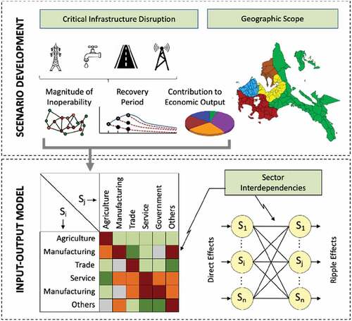
The impact of critical infrastructure sector failure caused by the volcanic eruption can be estimated through dynamic inoperability input-output modeling (DIIM). The Philippine National Disaster Risk Reduction Management Council (NDRRMC) publishes situational reports that provide information on damages and disruptions to economic and critical infrastructure sectors as well as their recovery. These are used as inputs for the DIIM to estimate the inoperability and economic losses that ripple through the regional economy. The framework for the current study is depicted in Figure 1. An exhaustive analysis of the data available in the 2020 Taal Volcano eruption situational report released by the government facilitated the development of study-specific scenarios describing the extent to which each infrastructure is disrupted as well as the length of the recovery period. This extracted information is then analyzed to evaluate the unique impacts on various economic sectors – knowing that each sector has different levels of dependence on the affected infrastructure. Using the DIIM, we simulated the ripple effects of infrastructure failure scenarios on the economic sectors of the study region to estimate a range of economic losses. The losses computed in this study are then validated with the results from other economic impact analysis studies pertaining to the Taal Volcano eruption.

Figure 1. Framework for integrating critical infrastructure disruption analysis with input-output model.

3. Integrated framework and application to the Taal Volcano eruption

3.1. Case study scenarios and data sources

This study considers the case of the Taal Volcano Eruption on 12 January 2020. The Philippine Institute of Volcanology and Seismology (PHIVOLCS) reported that Level 3 was raised in the surrounding communities at 8:00 AM (Philippine Institute of Volcanology and Seismology, 2022a). The study utilized the data provided in the situational report of the National Disaster Risk Reduction and Management Council (NDRRMC) on the effects of the volcanic eruption, which includes disruptions to infrastructure such as electric power, water, and land transportation in the nearby communities. Specifically, three provinces were affected, which are Cavite, Laguna, and Batangas. Such disruptions on the infrastructure systems have incurred significant economic costs and have posed challenges on the post-recovery of the affected areas. This is especially true since many communities around the Taal volcano are dependent on tourism economic activities. Figure 2 shows the map of study region. It can be observed that Taal Volcano is uniquely situated in Taal Lake. The 2020 Taal Volcano eruption was phreamagmatic in nature, causing a moderate to heavy level of ashfall as far as 70 kilometers north of Taal Volcano (Balangue-Tarriela et al., 2022).

Figure 2. Map of the study region.

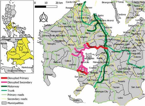
Figure 2 also presents the road network in the study region. Many roads were damaged and were closed due to the significant amount of ashfall. The red lines represent the unpassable primary roads and the pink lines represent the unpassable secondary roads. Primary roads are national roads that connect cities while secondary roads are directly connected to primary roads (Philippine Statistics Authority, n.d.). According to the National Disaster Risk Reduction and Management Council (2020) report, a total of 9 road sections were closed and needed debris/clearing operations. As a safety precaution, some of the roads were locked down. It was reported that 6 out of the 9 road sections were already passable as of last 30 January 2020. The remaining 3 road sections remained on lockdown. This significantly affected land transportation as many roads had to be closed off for safety reasons. Table 1 summarizes the road sections, their corresponding length in kilometers (km) and the average recovery period (in days). The study also does not consider in the estimation the roads that were unpassable at the time that the report was published. From the estimates, the initial inoperability level of the land transportation sector is 3%. The average recovery period for roads is 15 days after the volcanic eruption. Meanwhile, the standard deviation of the recovery period for roads is 0.88 days.

Table 1. Affected road sections, length of roads (in km) and average recovery period (in days).

Road Section	Length of Road (in km)	Average Recovery Period (in days)
Palico-Balayan-Batangas Road (Lemery Section), Batangas	5.53	15.33
Tanauan-Talisay-Tagaytay Road, Talisay-Tagaytay Section, Talisay, Batangas	22.07	15.33
Talisay Laurel-Agoncillo Road, Laurel Section, Batangas	20.00	15.33
Talisay Laurel-Agoncillo Road, Agoncillo Section, Batangas	11.98	17.42
K0114 + 254 – K0121 + 074, Batangas	6.82	16.29
K094 + 230 – K102 + 803, Batangas	8.57
K0100 + 026 – K102 + 803, Batangas	2.06
Tagaytay-Taal Lake Road, Tagaytay, Cavite	8.57	15.29
Tagaytay-Talisay Road, Tagaytay, Cavite	2.37
Total length of unpassable roads	87.97
Total length of roads in Region IV-A	3,038.76
Initial Inoperability for Land Transportation	3%
Average recovery period (in days)		15.83 $\approx$ 15
Standard deviation, $\sigma$		0.88

Source: National Disaster Risk Reduction and Management Council (2020) and authors’ calculations

Power supply in nearby cities and municipalities were also heavily affected by the Taal volcano eruption. National Disaster Risk Reduction and Management Council (2020) reported that there was a total of 23 cities/municipalities that experienced power interruption in the provinces of Cavite, Laguna, and Batangas. Table 2 shows the municipalities or cities per province that were affected, the number of households in each location, and the estimated average recovery period in days. Based on this, the estimate initial inoperability to be 19.5%, the average recovery period for power supply is 6 days and the standard deviation for the recovery period is estimated to be at 8.14 days.

Source: National Disaster Risk Reduction and Management Council (2020) and Philippine Statistics Authority (2022a).

Table 2. Power supply outages of the affected municipalities/cities per province, number of households in each location and estimated average recovery period (in days).

ProvinceMunicipality/City	Number of Households	Average recovery period (in days)
Cavite
Amadeo	10,317	6.13
Tagaytay City	22,399	6.13
Alfonso	14,556	4.06
Indang	17,012	4.06
Mendez	8,606	4.06
Laguna
Calamba	151,604	3.11
Cabuyao	100,875	4.50
Kalayaan	5,790	0.25
Lumban	8,535	0.13
Pagsanjan	11,404	0.23
Caviniti	6,300	0.17
Paete	5,883	0.23
Sta. Rosa	122,458	0.03
San Pedro	82,292	0.17
Batangas
Lipa City	89,993	17.00
Tanauan City	46,680	34.67
Laurel	9,626	4.17
Talisay	10,785	8.67
Lemery	21,122	17.00
Malvar	17,064	16.00
Balete	5,709	17.00
Sta. Teresita	5,547	4.00
Lian	15,991	4.00
Total Affected	790,548
Calabarzon Total	4,062,720
Initial Inoperability	19.5%
Average recovery period (in days):		6.39 $\approx \hspace{0.17em}$ 6.0
Standard deviation, $\sigma$		8.14

Source: National Disaster Risk Reduction and Management Council (2020) and Philippine Statistics Authority (2022a).

The National Disaster Risk Reduction and Management Council (2020) also reported that water supply in three cities/municipalities in the province of Batangas were affected. However, all the water supply services were restored by 29 January 2020. Table 3 shows the areas where water supply was disrupted, the number of households in each location, and the average recovery period (in days). The estimates suggest that the region suffered an initial inoperability of 0.9%, it takes at an average, 12.67 days after the volcanic eruption to restore the water supply services. The standard deviation of the recovery period for water supply is estimated at 6.66 days.

Table 3. Affected water supply, number of households and average recovery period (in days).

Municipality/City	Number of Households	Average Recovery Period (in days)
Laurel, Batangas	9,626	16
Talisay, Batangas	10,785	17
Taal, Batangas	14,977	5
Total Affected	35,388
CALABARZON Total	4,062,720
Initial Inoperability	0.9%
Average recovery period (in days)		12.7 $\approx$ 12
Standard deviation, $\sigma$		6.66

Source: National Disaster Risk Reduction and Management Council (2020) and authors’ calculations.

3.2. Dynamic inoperability input-output model

One of the significant contributions of this paper is the development of a spreadsheet-based graphical user interface (GUI) that utilizes the IO data¹ for the affected region. The GUI contains a blank table where users can directly populate the parameters pertaining to the initial inoperability (or level of dysfunctionality) of an infrastructure, as well as the recovery period (in days). Even with a moderately sized matrix comprising of 14 sectors (see, Table 4), the required computations are cumbersome since we must account for the impact of each infrastructure system on each economic sector and the dynamic behavior of inoperability over time. Recovery considers the inherent resilience of each sector and the coupling of each sector with other sectors. The GUI is customized for this study that features the region-specific data such as gross domestic product (GDP), sector-by-sector requirements, and production output, among others. Three infrastructure systems were included in the simulation: (a) electric power, (b) water, and (c) land transportation. Other infrastructure systems were excluded either because they are virtually unaffected (e.g., telecommunications) or non-existent in the directly affected area (e.g., air transportation). A pair of parameter inputs were required for each system, namely initial inoperability and recovery period. Such parameter inputs resulted from meticulous data extraction of scenarios as reflected in the situational report for the Taal Volcano eruption (National Disaster Risk Reduction and Management Council, 2020).

Table 4. Codes and descriptions of economic sectors used in the study.

Code	Sector Description
S01	Agriculture, Fishery and Forestry
S02	Mining and Quarrying
S03	Manufacturing
S04	Construction
S05	Electricity, Gas and Water
S06	Land Transportation
S07	Water Transport
S08	Air Transport
S09	Communications and Storage
S10	Trade
S11	Finance
S12	Real Estate and Ownership of Dwellings
S13	Private Services
S14	Government Services

3.2.1. Baseline scenario

Table 5 summarizes the initial inoperability and recovery periods that were computed based on the data extracted from the situational report and other data as discussed in the previous section. The inoperability parameter was based on the proportion of the region that experienced a disruption for a specific infrastructure. Furthermore, recovery period refers to the number of days the infrastructure is deemed to be operating back to a ‘business as usual’ levels. The recovery period data are not integer values (i.e., they contain decimal points); hence, we rounded them down to the nearest number of days to be compatible with the DIIM (i.e., as can be seen in the DIIM formulation in Eq. 2(2) ${\mathbf{q}}_{\mathrm{t}+1}={\mathbf{q}}_{\mathrm{t}}+\mathbf{K}\left[{\mathbf{A}}^{\ast }{\mathbf{q}}_{\mathrm{t}}+{\mathbf{c}}_{\mathrm{t}}^{\ast }-{\mathbf{q}}_{\mathrm{t}}\right]$(2) , the time increments are discrete).

Table 5. Direct disruption inputs to the DIIM based on taal volcano situation reports (Baseline scenario).

Infrastructure System	Initial Inoperability (%)	Recovery Period (days)
(a) Electric Power	19.5	6
(b) Water	0.9	12
(c) Land Transportation	3	15

Using the input data in Table 5, each infrastructure disruption scenario was simulated using the DIIM GUI. Hence, three separate simulations were performed each for (a) electric power, (b) water, and (c) land transportation. The plots in Figure 3 depict the inoperability (left panel) and economic loss (right panel) results because of separate disruptions in the three infrastructure systems. The details of the analysis are deferred to the subsequent sections when the results for all three infrastructure systems are aggregated. Nonetheless, several high-level observations can be made from Figure 3.

Figure 3. Inoperability and economic loss results for each infrastructure disruptions (Baseline scenario).

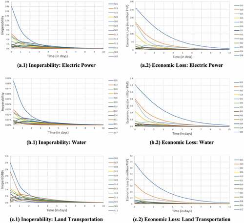
First, the sector rankings for inoperability and economic loss are different even if the disruption is caused by the same infrastructure. Looking at the first row of Figure 3, the most affected sector in terms of inoperability is S05 (electricity, gas, and water), while the most affected sector in terms of economic loss is S03 (manufacturing). This is because inoperability typically measures the percentage disruption to the sector and since electric power is the one being disrupted here, it only makes sense that the worst inoperability occurs in the overarching sector that encompasses electric power distribution. For economic loss, the manufacturing sector is the most affected because this sector not only relies heavily on electric power but also because it is the sector with the highest contribution to the GDP.

Secondly, performing a cross-comparison between electric power and water disruptions (first and second rows in Figure 3), the sector rankings for inoperability are similar (left panel). The same can be said about the similarity in economic loss rankings when electric power and water disruptions are compared (right panel). This is due to a data limitation for the IO matrix used in the study where electric power and water are aggregated within the same economic sector. Nonetheless, we were able to disaggregate the initial inoperability and recovery inputs that enabled us to assess the significant losses that are attributable to the electric power. Looking at the y-axis of electric power vs the y-axis of water (right panel), one can conclude that the economic losses due to electric power disruption is significantly higher in contrast to the economic losses due to water disruption. The breakdown of the losses will be reported later in this paper.

Third, doing a cross-comparison between electric power and land transportation disruptions (first and third rows in Figure 3), the sector rankings are markedly different for both inoperability and economic loss measures. This is because electric power and land transportation have separate overarching sectors (S05 and S06, respectively). For land transportation disruption, the land transportation sector (S06) ranks as the most affected sector in both inoperability and economic loss. It can also be noted that in the third row right panel that manufacturing sector (S03) is the second most affected sector in terms of economic loss. For the inoperability rankings in land transportation (third row, left panel), it can be observed that the inoperability trajectories of the other sectors are much lower than that of the land transportation sector itself. It is worth noting that resilience-enhancing strategies have been creatively implemented in the region such that it is able to continue transporting products on partially damaged roads and dirt roads using smaller vehicles like motorcycles. As a matter of fact, at the height of the pandemic in the Philippines, product deliveries using motorbikes (e.g., Grab) and small trucks and vans (e.g., Lalamove) have boomed exponentially and become ubiquitous in the Philippines (Abadilla, 2020).

More importantly, this paper focuses on the resulting inoperability and economic loss experienced in the region when all three infrastructure system disruptions occurred simultaneously. When computed and aggregated, the economic losses due to simultaneous infrastructure disruptions can be validated subsequently with estimates from other independent sources.

The plot and ranking of the most affected sectors using the inoperability measure are shown in Figure 4 and Table 6 respectively.

Figure 4. Inoperability results for combined critical infrastructure disruptions (Baseline scenario).

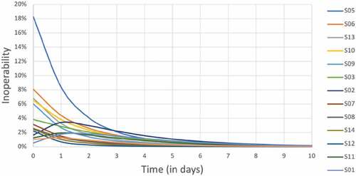
Table 6. Inoperability rankings for combined infrastructure rankings (Baseline scenario).

Most Affected Sectors		Peak Inoperability (%)
S05	Electricity, Gas and Water	17.81%
S06	Land Transportation	7.95%
S13	Private Services	6.67%
S10	Trade	6.39%
S09	Communications and Storage	5.90%
S03	Manufacturing	3.76%
S02	Mining and Quarrying	3.35%
S07	Water Transport	3.12%
S08	Air Transport	2.58%
S14	Government Services	2.41%
S12	Real Estate and Ownership of Dwellings	2.17%
S11	Finance	1.90%
S01	Agriculture, Fishery and Forestry	1.78%
S04	Construction	1.22%

Note that while most of the sectors have monotonically decreasing inoperability functions, there are several exceptions. A case is the mining and quarrying sector (S02) where the inoperability increases at the onset of the disruption and decreases after reaching its peak. Other sectors that experience an initial increase in inoperability are the finance sector (S11), construction sector (S04) and the agriculture, fishery and forestry sector (S01). These sectors are strongly dependent on the disrupted sectors thereby resulting to initially increasing levels of inoperability. The sectors are ranked according to their peak inoperability, which is shown in the table below. The top-ranked sectors are evidently the same sectors that encompass the infrastructure systems from which the direct disruptions originated, namely land transportation (S06) and electricity, gas, and water (S05). The remainder of the rankings are shown in the table below, indicating significant indirect inoperability impacts on sectors that rely heavily on the disrupted systems. The next three sectors reached double-digit peak inoperability values including S13 (private services), S10 (trade), and S09 (communications and storage). Consulting the table below, it is evident that all economic sectors become inoperable at varying levels depending on their dependence on electric power, water, and land transportation infrastructure systems. At the bottom of the ranking is construction, which suffered a 1.22% inoperability.

Furthermore, the plot and ranking for the economic loss measure are shown in Figure 5 and Table 6, respectively. Most of the sectors have monotonically decreasing loss functions, except for a few such as the light blue curve S01 (agriculture, fishery, and forestry), where economic loss peaks sometime after day 1 and dissipates thereafter. It can also be observed that the agriculture, fishery, and forestry sector suffers the fifth highest loss, and this is intuitive since this sector is economically significant in the study region.

Figure 5. Economic loss results for combined critical infrastructure disruptions (Baseline scenario).

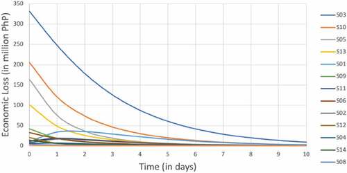
Table 7 shows the breakdown of economic losses for the affected economic sectors ranked from highest to lowest. The top 3 sectors incurred a combined loss of about PhP 1,982 million, and these sectors are manufacturing (S03), trade (S10), and electricity, gas, and water (S05), accounting for more than 70% of the total loss of PhP 2,800 million. Interestingly, the loss of the top 2 sectors are purely indirect effects due to their reliance on the directly affected infrastructure systems. The most impacted sector, manufacturing sector (S03), the sector with the highest GDP contribution to the region suffered a loss of PhP 1141 million. The region is also heavily involved in trading; hence, it is not surprising that the trade sector suffered the second largest economic loss amounting to PhP 527 million. The third largest loss amounted to PhP 314 million, which was suffered by the electricity, gas, and water sector (S05). The remainder of the economic loss breakdown for each sector is enumerated in Table 7. All sectors suffered varying levels of economic loss, with water transport sector suffering the least loss of PhP 2 million. This result is consistent with situational report findings that indicate there was a minimal impact on water transport activities in the region.

Table 7. Economic losses rankings for combined infrastructure rankings (Baseline scenario).

Most Affected Sectors		Economic Loss (in million PhP)
S03	Manufacturing	1,141
S10	Trade	527
S05	Electricity, Gas and Water	314
S13	Private Services	214
S01	Agriculture, Fishery and Forestry	181
S09	Communications and Storage	85
S11	Finance	83
S06	Land Transportation	80
S02	Mining and Quarrying	74
S12	Real Estate and Ownership of Dwellings	32
S04	Construction	30
S14	Government Services	28
S08	Air Transport	9
S07	Water Transport	2
Total Economic Loss		2,800

3.2.2. Sensitivity analysis

In the previous section, we simulated the ripple effects of infrastructure disruptions based on the baseline values of the model parameters as shown in Table 5. In this section, we will introduce two additional scenarios as depicted in Table 8. From Section 3.1, we provided the calculations for the initial inoperability values for the three infrastructure systems. Furthermore, for the recovery period parameters, we created a new pessimistic scenario in which the recovery period for each infrastructure would exceed the baseline. We calculated the standard deviation ($\sigma$) of the recovery period data and assumed that the pessimistic value corresponds to a $1\sigma$ exceedance. The standard deviation values have also been provided in Section 3.1. Note that this sensitivity analysis focuses on the increase in recovery period. As such, the same initial inoperability values were applied in both the baseline and pessimistic scenarios.

Table 8. Parameters used for sensitivity analysis of initial inoperability and recovery period.

Scenario Infrastructure	Initial Inoperability (%)		Recovery Period (days)
	Baseline	Pessimistic	Baseline	Pessimistic
(a) Electric Power	19.5	19.5	6	14
(b) Water	0.9	0.9	12	19
(c) Land Transportation	3	3	15	16

For the new pessimistic scenario, the breakdown of inoperability values is presented in Table 9. Note that since the initial inoperability parameters are the same as with the baseline case – albeit with slightly longer recovery periods – we can observe from comparison of Table 9 and Table 6 that the first 11 highest-ranked sectors have essentially the same peak inoperability values as the ones reported in the baseline case. Nonetheless, the last 3 lowest-ranked sectors in the pessimistic scenario have lower peak inoperability values compared to their baseline counterparts, which is counterintuitive. While the peak inoperability values are lower in the pessimistic scenario, it should be noted that the duration of time that the sectors remain in the peak inoperability levels is longer due to the extended recovery time, resulting in higher-order indirect impacts. Longer recovery period will subsequently result in higher economic losses as will be reflected in the discussions surrounding Table 10.

Table 9. Inoperability rankings for combined infrastructure rankings (Pessimistic scenario).

Most Affected Sectors		Peak Inoperability (%)
S05	Electricity, Gas and Water	17.81%
S06	Land Transportation	7.95%
S13	Private Services	6.67%
S10	Trade	6.39%
S09	Communications and Storage	5.90%
S03	Manufacturing	3.76%
S07	Water Transport	3.12%
S02	Mining and Quarrying	3.00%
S08	Air Transport	2.58%
S14	Government Services	2.41%
S12	Real Estate and Ownership of Dwellings	2.17%
S11	Finance	1.76%
S01	Agriculture, Fishery and Forestry	1.70%
S04	Construction	1.17%

Table 10. economic losses rankings for combined infrastructure rankings (Pessimistic scenario).

Most Affected Sectors		Economic Loss (in million PhP)
S03	Manufacturing	1,445
S10	Trade	668
S05	Electricity, Gas and Water	398
S13	Private Services	271
S01	Agriculture, Fishery and Forestry	230
S09	Communications and Storage	108
S11	Finance	105
S06	Land Transportation	101
S02	Mining and Quarrying	94
S12	Real Estate and Ownership of Dwellings	41
S04	Construction	38
S14	Government Services	35
S08	Air Transport	12
S07	Water Transport	2
Total Economic Loss =		3,546

The breakdown of economic loss values for the pessimistic scenario is presented in Table 10. While the rankings are the similar compared with the baseline case in Table 5, it can be observed that the values of economic losses are significantly higher compared with the baseline values. For example, manufacturing suffered PhP 1,445 million in the pessimistic scenario (see, Table 10), in contrast to the PhP 1141 million it suffered in the baseline scenario (see, Table 7). While some of the peak inoperability values were lower for the pessimistic scenario relative to the baseline scenario, the reason why the economic loss is much higher is that the prolonged recovery period kept the sector longer in the peak inoperability region. The rest of the sectors also suffered higher economic loss values when the pessimistic scenario is juxtaposed with the corresponding values in the baseline scenario.

3.3. Summary of results for the two scenarios

Table 11 summarizes the inoperability and economic loss rankings, respectively, for the two scenarios. Scenario 1 corresponds to the baseline column, while Scenario 2 corresponds to the pessimistic column. Most of the analyses for the two scenarios have been discussed separately in the previous sections and will not be repeated here. Nonetheless, there are main takeaway points that need to be reemphasized as follows:

• The rankings of inoperability and economic loss are different; and both rankings must be considered when implementing policy decisions pertaining to resource allocation.

• The baseline and pessimistic values present a possible range of values adhering to the need for uncertainty analysis required when making estimates of disaster losses.

• Sensitivity analysis revealed that the total economic losses (see last row of Table 11) can range between PhP 2.8 billion to PhP 3.5 billion.

• The estimated economic loss (see last row of Table 11) is aligned with the official estimated loss of PhP 4.8 billion as published by the National Economic and Development Authority Region IV-A (2020) such that the lower estimates presented in Table 11 excludes the initial inoperability in the agriculture, fishery and forestry sector.

Table 11. Economic loss rankings the two scenarios in thousand PHP.

Most Affected Sectors		Scenario 1: Baseline	Scenario 2: Pessimistic
S06	Manufacturing	1,141	1,445
S05	Trade	527	668
S13	Electricity, Gas and Water	314	398
S10	Private Services	214	271
S09	Agriculture, Fishery and Forestry	181	230
S02	Land Transportation	85	108
S03	Communications and Storage	83	105
S12	Finance	80	101
S14	Mining and Quarrying	74	94
S11	Real Estate and Ownership of Dwellings	32	41
S01	Construction	30	38
S04	Government Services	28	35
S07	Air Transport	9	12
S08	Water Transport	2	2
Total Economic Loss (in million PhP)		2,800	3,546

4. Conclusions and areas for future research

In this paper, we developed and customized the classical economic I-O model for estimating the direct and indirect ripple effects due to the eruption of Taal Volcano in the Philippines. This disaster affected primarily the provinces of Cavite, Laguna, and Batangas in the island of Luzon, which is the largest island of the Philippines. Although the region is contiguous to the Philippine National Capital Region, the spillover effects were fortunately minimal; hence the losses estimated in this paper are only focused on the directly affected provinces and municipalities (see, Figure 2, Tables 1– 3).

The direct effects were caused mainly by disrupted critical infrastructure systems such as electric power, water, and land transportation. These are the systems that were heavily impacted in the region. While there are other types of critical infrastructure systems, they are either practically non-existent in the region (e.g., air and water transport) or minimally disrupted due to their higher resilience (e.g., communications and storage). In modeling the infrastructure disruptions, we calculated the dependence of each economic sector on the affected infrastructure and simulated the trajectory of inoperability given the recovery periods available in a government-released situational report. Inoperability is a dimensionless measure of the proportional extent to which an infrastructure’s functionality is disrupted relative to its ideal operation.

Different municipalities suffered varying levels of inoperability and we calculated the weighted average of both the initial inoperability and recovery time, considering the significance of the infrastructure and the number of affected populations in each municipality. Given these input parameters, we simulated the dynamics of the recovery for the affected economic sectors. Since the IO data for the Philippines is typically available at the national scale, this paper developed an IO table customized for the region, comprising of 14 sectors (see, Table 2).

A graphical user interface (GUI) for the dynamic inoperability input-output model, or DIIM, was developed and deployed in this study. The GUI has a simple interface where users can enter different combinations of initial inoperability and recovery period values. After these model parameters are entered, the DIIM automatically calculates and provides visualizations of the inoperability and economic loss for each sector over the recovery horizon. The resulting plots are accompanied by a table containing the ranking of sectors based on the inoperability and economic loss measures. These two measures generate different sector rankings. Inoperability typically focuses on the sectors that – albeit their relatively low contribution to the GDP – can potentially create more cascading effects and consequently can further lengthen the recovery. Economic loss, on the other hand, reflects the monetary worth of damage incurred in each sector. Together, these two measures can provide a more robust guidance pertaining to resource allocation decisions.

For this study, sectors that were found to have the highest peak inoperability include electricity, gas, and water, land transportation, private services, and trade, to name a few. It is intuitive that the two most affected sectors are the same sectors that encompass the initially affected infrastructure systems. Private services and trade were also among the sectors that suffered the brunt of the inoperability measure, and this result is intuitive since these sectors are heavily dependent primarily on electric power and land transportation.

In contrast, the sectors that incurred the highest economic losses include manufacturing, trade, electricity, gas and water, private services, and agriculture, fishery and forestry. Manufacturing is the largest GDP contributor in the region and it comes with no surprise that it also suffered the highest economic loss, accounting for nearly 40% of the total economic loss for the region. It is also worth noting that the region is resource rich and heavily engaged in agricultural activities, hence making this sector also vulnerable to the eruption. For the case study, we simulated two different scenarios (baseline, and pessimistic) to generate a range of economic loss estimates, which we estimated to be somewhere between PhP 2.8–3.5 billion.² As a validation, we have found that our estimates are consistent as other independent studies, which estimated the losses at PhP 4.8 billion which includes initial inoperability in the agriculture, fishery and forestry sector (NEDA Region IV-A, 2020).

While our results matched the official estimates, there are assumptions and limitations that can further refine the analysis. Taal Volcano, one of the world’s smallest volcanoes blanketed by the picturesque Taal Lake, attracts many tourists both domestic and foreign. Within the regional I-O data, the tourism industry is heavily aggregated within the private services sector and it is difficult to extract it separately to estimate its contribution to the economic loss. However, the Taal Volcano eruption occurred during an off-peak season, and we argue that the loss to the tourism industry would have been far greater had it happened during the holidays or the summer peak season. Other extensions that can be revisited in the future include the costs associated with evacuation of displaced populations, productivity losses due to degraded morale and post-traumatic stress disorder, as well as the medical costs associated with illnesses and deaths – which are beyond the economic loss scope of the current study.

In conclusion, the I-O based methodology and companion decision support system developed in this paper can serve as a template for future studies to estimate the ripple effects of infrastructure failures to interdependent economic sectors. Our model and analysis prescribe different dimensions of prioritization. Typically, policymakers are primarily concerned with keeping economic losses to a minimum. Nonetheless, such one-dimensional mindset has the tendency to leave out sectors with relatively low contribution to the GDP but are critical to expediting the recovery process. As such, a myopic or short-term focus on economic loss reduction can potentially create a paradox of neglecting other sectors that could be pivotal to the recovery process – ironically generating more losses in the long run. Hence, sensitivity analysis such as the ones performed in the study is needed to enhance the robustness of the prioritization process that consider other metrics such as peak inoperability, resilience and its impact on recovery period, and the degree and complexity of the coupling amongst the sectors. Examples of resilience strategies that can be further explored include excess inventory in anticipation of a disaster, production recapture (e.g., employee overtimes to compensate for loss of production), facility relocation, building up buffer capacity, among others. Hence, a future topic can investigate the cost-effectiveness and impact of such resilience tactics on economic loss reduction and the enhanced pace of regional recovery.

Disclosure statement

The Coalition for Disaster Resilient Infrastructure (CDRI) reviewed the anonymised abstract of the article, but had no role in the peer review process nor the final editorial decision.

Additional information

Funding

This work was supported by the US National Science Foundation [1832635], Fulbright US Scholar Program, and Philippine-American Educational Foundation (PAEF). The Article Publishing Charge (APC) for this article is funded by the Coalition for Disaster Resilient Infrastructure (CDRI).

Notes

¹ The input-output table of Region IV-A (CALABARZON Region), for 2019 was estimated using location quotient approach (Miller & Blair, 2009) based on the 2012 Philippine Input-Output Table (Philippine Statistics Authority, 2017) calibrated with the 2019 regional gross domestic product (Philippine Statistics Authority, 2022b).

² As a reference, in year 2020, USD 1 is approximately PhP 50; hence the economic losses vary between USD 56-70 million.

References

- Abadilla, E. V. (2020, August 2). Delivery firms big winners in quarantine. Manila Bulletin. https://mb.com.ph/2020/08/02/delivery-firms-big-winners-in-quarantine/
- Allen, W., Cruz, J., & Warburton, B. (2017, March). How Decision Support Systems Can Benefit from a Theory of Change Approach. Environmental Management, 59, 956–965. https://doi.org/10.1007/s00267-017-0839-y
- Asano, T., & Nagayama, A. (2021). Analysis of workload required for removal of drifting pumice after a volcanic disaster as an aspect of a port business continuity plan: A case study of Kagoshima port, Japan. International Journal of Disaster Risk Reduction, 64(October 2021), 102511. https://doi.org/10.1016/j.ijdrr.2021.102511
- Aven, T., Ben-Haim, Y., Andersen, H. B., Cox, T., Droguett, E. L., Greenberg, M., Guikema, S., Kröger, W., Renn, O., Thompson, K., & Zio, E. (2018). Society for risk analysis glossary. https://www.sra.org/wp-content/uploads/2020/04/SRA-Glossary-FINAL.pdf
- Baghersad, M., & Zobel, C. W. (2015). Economic impact of production bottlenecks caused by disasters impacting interdependent industry sectors. International Journal of Production Economics, 168(October 2015), 71–80. https://doi.org/10.1016/j.ijpe.2015.06.011
- Balangue-Tarriela, M. I. R., Lagmay, A. M. F., Sarmiento, D. M., Vasquez, J., Baldago, M. C., Ybañez, R., Ybañez, A. A., Trinidad, J. R., Thivet, S., Gurioli, L., Van Wyk de Vries, B., Aurelio, M., Rafael, D. J., Bermas, A., & Escudero, J. A. (2022). Analysis of the 2020 Taal Volcano tephra fall deposits from crowdsoured information and field data. Bulletin of Volcanology, 84(35), 1–22. https://doi.org/10.1007/s00445-022-01534-y
- Barker, K., & Santos, J. R. (2010). Measuring the efficacy of inventory with a dynamic input output model. International Journal of Production Economics, 126(1), 130–143. https://www.sciencedirect.com/science/article/abs/pii/S092552730900293X?via/3Dihub
- Budd, L., Griggs, S., Howarth, D., & Ison, S. (2011). A fiasco of volcanic proportions? Eyjafjallajökull and the closure of European airspace. Mobilities, 6(1), 31–40. https://doi.org/10.1080/17450101.2011.532650
- Delos Reyes, P. J., Bornas, M. A. V., Dominey-Howes, D., Pidlaoan, A. C., Magill, C. R., & Solidum, R. U. (2018). A synthesis and review of historical eruptions at Taal Volcano, Southern Luzon. Philippines, Earth-Science Reviews, 177(B6), 565–588. https://doi.org/10.1016/j.earscirev.2017.11.014
- Echegaray-Aveiga, R. C., Rodríguez-Espinosa, F., Toulkeridis, T., & Echegaray-Aveiga, R. D. (2020). Possible effects of potential lahars from Cotopaxi volcano on housing market prices. Journal of Applied Volcanology, 9(1), 4. https://doi.org/10.1186/s13617-020-00093-1
- Eling, M., Elvedi, M., & Falco, G. (2022). The economic impact of extreme cyber risk scenarios. North American Actuarial Journal, 1–15. https://doi.org/10.1080/10920277.2022.2034507
- Frazier, T. G., Thompson, C. M., Dezzani, R. J., & Butsick, D. (2013). Spatial and temporal quantification of resilience at the community scale. Applied Geography, 42(August 2013), 95–107. https://doi.org/10.1016/j.apgeog.2013.05.004
- Galbusera, L., & Giannopoulos, G. (2018). On input-output economic models in disaster impact assessment. International Journal of Disaster Risk Reduction, 30(Part B, September 2018), 186–198. https://doi.org/10.1016/j.ijdrr.2018.04.030
- Haimes, Y. Y. (1991). Total risk management. Risk Analysis, 11(2), 169–171. https://doi.org/10.1111/j.1539-6924.1991.tb00589.x
- Haimes, Y. Y., Horowitz, B. M., Lambert, J. H., Santos, J. R., Lian, C., & Crowther, K. G. (2005). Inoperability input-output model for interdependent infrastructure sectors. I: Theory and methodology. Journal of Infrastructure Systems, 11(2), 67–79. https://doi.org/10.1061/(ASCE)1076-0342(2005)11:2(67)
- Haimes, Y. Y., & Jiang, P. (2001). Leontief-based model of risk in complex interconnected infrastructures. Journal of Infrastructure Systems, 7(1), 1–12. https://doi.org/10.1061/(ASCE)1076-0342(2001)7:1(1)
- Hayes, J. L., Biass, S., Jenkins, S. F., Meredith, E. S., & Williams, G. T. (2022). Integrating criticality concepts into road network disruption assessments for volcanic eruptions. Journal of Applied Volcanology, 11(1), 8. https://doi.org/10.1186/s13617-022-00118-x
- Hermon, D., Ganefri, E., Iskarni, P., & Syam, A. (2019). A Policy Model of Adaptation Mitigation and Social Risks the Volcano Eruption Disaster of Sinambung in Karo Regency-Indonesia”. International Journal of Geomate, 17(60), 190–196. https://doi.org/10.21660/2019.60.50944
- Hynes, W., Trump, B. D., Kirman, A., Haldane, A., & Linkov, I. (2022). Systemic resilience in economics. Nature Physics, 18(4), 381–384. https://doi.org/10.1038/s41567-022-01581-4
- Imamura, F., Suppasri, A., Arikawa, T., Koshimura, S., Satake, K., & Tanioka, Y. (2022). Preliminary observations and impact in Japan of the tsunami caused by the Tonga Volcanic eruption on January 15, 2022. Pure and Applied Geophysics, 179(5), 1549–1560. https://doi.org/10.1007/s00024-022-03058-0
- International Organization for Migration and Department of Social Welfare and Development. (2020). Displacement tracking matrix: Philippines – Taal Volcano eruption (Report No. 2).
- Jena, R., Pradan, B., Beydoun, G., Al-Amri, A., & Sofyan, H. (2020). Seismic hazard and risk assessment: A review of the state-of-the-art traditional and GIS models. Arabian Journal of Geosciences, 13(2), 50. https://doi.org/10.1007/s12517-019-5012-x
- Jonkeren, O., & Giannopoulos, G. (2014). Analysing critical infrastructure failure with a resilience inoperability input-output model. Economic Systems Research, 26(1), 39–59. https://doi.org/10.1080/09535314.2013.872604
- Jumadi, J., Malleson, N., Carver, S., & Quincey, D. (2020). Estimating spatio-temporal risks from volcanic eruptions using an agent-based model. Journal of Artificial Societies and Social Simulation, 23(2), 2. https://doi.org/10.18564/jasss.4241
- Kaplan, S., & Garrick, B. J. (1981). On the quantitative definition of risk. Risk Analysis, 1(1), 11–27. https://doi.org/10.1111/j.1539-6924.1981.tb01350.x
- Kazantzidou-Firtinidou, D., Kassaras, I., & Ganas, A. (2018). Empirical seismic vulnerability, deterministic risk and monetary loss assessment in Fira (Santorini, Greece). Natural Hazards, 93(3), 1251–1275. https://doi.org/10.1007/s11069-018-3350-8
- Kim, J., Nakano, S., & Nishimura, K. (2021). The role of ICT productivity in Korea-Japan multifactor CES productions and trades. Applied Economics, 53(14), 1613–1627. https://doi.org/10.1080/00036846.2020.1841084
- Kim, K., Pant, P., Yamashita, E., & Ghimire, J. (2019). Analysis of transportation disruptions from recent flooding and volcanic disasters in Hawaii. Environment, Planning and Climate Change, 2673(2), 194–208. https://doi.org/10.1080/00036846.2020.1841084
- La Porte, T. M. (2006). Managing for the unexpected: Reliability and organizational resilience. In P. E. Auerswald, L. M. Branscomb, T. M. La Porte, & E. O. Michel-Kerjan (Eds.), Seeds of disaster, roots of response: How private action can reduce public vulnerability (pp. 71–76). Cambridge University Press; 1st edition (September 18, 2006). https://doi.org/10.1017/CBO9780511509735.008
- Leontief, W. W. (1936). Quantitative input and output relations in the economic systems of the United States. The Review of Economics and Statistics, 18(3), 105–125. https://doi.org/10.2307/1927837
- Leung, M. F., Santos, J. R., & Haimes, Y. Y. (2003). Risk modeling, assessment, and management of lahar flow threat. Risk Analysis, 23(6), 1323–1335. https://doi.org/10.1111/j.0272-4332.2003.00404.x
- Lewandowski, A., & Wierzbicki, A. P. (1989). Aspiration based decision support systems: Theory, software, and applications. Springer Science & Business Media, (Lecture Notes in Economics and Mathematical Systems, 331) 1st Edition, 331, 1–21.
- Lian, C., & Haimes, Y. Y. (2006). Managing the risk of terrorism to interdependent infrastructure systems through the dynamic inoperability input–output model. Systems Engineering, 9(3), 241–258. https://doi.org/10.1002/sys.20051
- MacKenzie, C. A., & Barker, K. (2013). Empirical data and regression analysis for estimation of infrastructure resilience with application to electric power outages [Article]. Journal of Infrastructure Systems, 19(1), 25–35. https://doi.org/10.1061/(ASCE)IS.1943-555X.0000103
- Manila Water. (n.d.) Special report: Taal Volcano eruption. https://reports.manilawater.com/2020/special-reports/taal-volcano-eruption
- McDonald, G. W., Smith, N. J., Kim, J.-H., Cronin, S. J., & Proctor, J. N. (2017). The spatial and temporal ‘cost’ of volcanic eruptions: Assessing economic impact, business inoperability, and spatial distribution of risk in the Auckland region. New Zealand, Bulletin of Volcanology, 79(7), 48. https://doi.org/10.1007/s00445-017-1133-9
- Merin, E. J. G., Yute, A. L. F., Sarmiento, C. J. S., & Elazagui, E. E. (2021). Ashfall dispersal mapping of the 2020 taal volcano eruption using diwata-2 imagery for disaster assessment. International Archives of the Photogrammetry, Remote Sensing and Spatial Information Sciences - ISPRS Archives, 46(4/W6–2021), 221–226. https://doi.org/10.5194/isprs-archives-XLVI-4-W6-2021-221-2021
- Miller, R. E., & Blair, P. D. (2009). Input-output analysis: Foundations and extensions (2nd ed.). Cambridge University Press, NJ.
- Monge, J. J., McDonald, N., & McDonald, G. W. (2022). A review of graphical methods to map the natural hazard-to-wellbeing risk chain in a socio-ecological system. Science of the Total Environment, 803(10 January 2022), 149947. https://doi.org/10.1016/j.scitotenv.2021.149947
- Murdock, H. J., De Bruijn, K. M., & Gersonius, B. (2018). Assessment of critical infrastructure resilience to flooding using a response curve approach. Sustainability, 10(10), 3470. https://doi.org/10.3390/su10103470
- National Disaster Risk Reduction and Management Council. (2020). NDRRMC update (Situational Report No. 87 re Taal Volcano eruption). https://ndrrmc.gov.ph/attachments/article/4007/Sitrep_No_87_re_Taal_Volcano_Eruption_as_of_06March2020_8AM.pdf
- National Economic and Development Authority Region IV-A. (2020). Rehabilitation and recovery program for Taal Volcano eruption affected areas.
- National Electrification Administration (2020, January 14). NEA: Forced power outage imposed in batangas towns due to Taal eruption. https://www.nea.gov.ph/ao39/517-nea-forced-power-outage-imposed-in-batangas-towns-due-to-taal-eruption
- Orencio, P. M., & Fujii, M. (2013). A localized disaster-resilience index to assess coastal communities based on an analytical hierarchy process (AHP). International Journal of Disaster Risk Reduction, 3(March 2013), 62–75. https://doi.org/10.1016/ssj.ijdrr.2012.11.006
- Pagsuyoin, S., Santos, J., Salcedo, G., & Yip, C. (2019). Spatio-temporal drought risk analysis using GIS-based input output modeling. In O, Yasuhide & R, Adam (ed.), Advances in spatial and economic modeling of disaster impacts (pp. 375–397). Springer.
- Papale, P., & Papale, P. (2019). Volcanic threats to global society. Science, 363(6433), 1275–1276. https://doi.org/10.1126/science.aaw7201
- Paté-Cornell, E. (2002). Finding and fixing systems weaknesses: Probabilistic methods and applications. Risk Analysis, 22(2), 319–334. https://doi.org/10.1111/0272-4332.00025
- Peers, J. B., Gregg, C. E., Lindell, M. K., Pelletier, D., Romerio, F., & Joyner, A. T. (2021). The economic effects of volcanic alerts — A case study of high-threat U.S. volcanoes. Risk Analysis, 41(10), 1759–1781. https://doi.org/10.1111/risa.13702
- Philippine Institute of Volcanology and Seismology. (2022a, March 26). Taal Volcano Eruption update 26 March 2022 07:45 PM. https://www.phivolcs.dost.gov.ph/index.PHP/volcano-hazard/volcano-bulletin2/taal-volcano/14331-taal-volcano-eruption-update-26-march-2022-07-45-pm
- Philippine Institute of Volcanology and Seismology. (2022b, August 12). Taal volcano advisory. https://www.phivolcs.dost.gov.ph/index.PHP/volcano-advisory-menu/15464-taal-volcano-advisory-12-august-2022-09-00-a-m
- Philippine Institute of Volcanology and Seismology. (n.d.) Philippine volcanoes (Ongoing audit). https://wovodat.phivolcs.dost.gov.ph/volcano/ph-volcanoes
- Philippine Statistics Authority. (2017). 2012 input-output tables – transaction table. https://psa.gov.ph/sites/default/files/2012%20Input-Output%20Tables%20-%20Transaction%20Table.xlsx
- Philippine Statistics Authority. (2022a). Household population, number of households, and average household size of the Philippines (2020 census of population and housing). https://psa.gov.ph/sites/default/files/attachments/hsd/pressrelease/3_Tables%201-2_TotPop%2C%20HHPop%2C%20HHs%2C%20and%20AHS_RML_032122_rev_RRDH_CRD.xlsx
- Philippine Statistics Authority. (2022b). 2000-2021 gross regional domestic product. https://psa.gov.ph/sites/default/files/GRDP_Reg_2018PSNA_2000-2021.xlsx
- Reyes-Hardy, M.-P., Aguilera Barraza, F., Sepúlveda Birke, J. P., Esquivel Cáceres, A., & Inostroza Pizarro, M. (2021). GIS-based volcanic hazards, vulnerability and risks assessment of the Guallatiri Volcano, arica y parinacota region, Chile. Journal of South American Earth Sciences, 109(August 2021), 103262. https://doi.org/10.1016/j.jsames.2021.103262
- Roquel, K. I. D., Fillone, A., & Yu, K. D. (2019). Comparative flood-risk assessment of different freight transport development programs. DLSU Business and Economics Review, 29(1), 146–164. https://dlsuber.com/wp-content/uploads/2019/08/13.pdf
- Rose, A. (2007). Economic resilience to natural and man-made disasters: Multidisciplinary origins and contextual dimensions. Environmental Hazards, 7(4), 383–398. https://doi.org/10.1016/j.envhaz.2007.10.001
- Saltos-Rodriguez, M., Aguirre-Velasco, M., Velasquez-Lozano, A., Villamarin-Jacome, A., Haro, J. R., & Ortiz-Villalba, D. (2021). Resilience assessment in electric power systems against volcanic eruptions: Case on lahars occurrence. IEEE Green Technologies Conference, 305–311.
- Santos, J. R., & Haimes, Y. Y. (2004). Modeling the demand reduction input‐output (I‐O) inoperability due to terrorism of interconnected infrastructures. Risk Analysis: An International Journal, 24(6), 1437–1451. https://doi.org/10.1111/j.0272-4332.2004.00540.x
- Santos, J. R., Orsi, M. J., & Bond, E. J. (2009). Pandemic recovery analysis using the dynamic inoperability input‐output model. Risk Analysis: An International Journal, 29(12), 1743–1758. https://doi.org/10.1111/j.1539-6924.2009.01328.x
- Santos, J. R., Pagsuyoin, S. T., Herrera, L. C., Tan, R. R., & Yu, K. D. (2014). Analysis of drought risk management strategies using dynamic inoperability input–output modeling and event tree analysis. Environment Systems and Decisions, 34(4), 492–506. https://doi.org/10.1007/s10669-014-9514-5
- Shroder, J. F., & Papale, P. (eds). (2015). Volcanic hazards, risks, and disasters. Elsevier.
- Taghizadeh, O., Abbas, Ardalan, A., Paton, D., Jabbari, H., & Khankeh, H. R. (2015). Community Disaster Resilience: A Systematic Review on Assessment Models and Tools. PLoS Currents, 7. https://doi.org/10.1371/currents.dis.f224ef8efbdfcf1d508dd0de4d8210ed
- Tiboldo, G., Boehm, R., Shah, F., Moro, D., & Castellari, E. (2022). Taxing the heat out of the US food system. Food Policy, 110(July 1), 102266. https://doi.org/10.1016/j.foodpol.2022.102266
- Trump, B. D., Linkov, I., & Hynes, W. (2020). Combine resilience and efficiency in post-COVID societies. Nature, 588(7837), 220–221. https://doi.org/10.1038/d41586-020-03482-z
- Wilson, T. M., Stewart, C., Sword-Daniels, V., Leonard, G. S., Johnston, D. M., Cole, J. W., Wardman, J., Wilson, G., & Barnard, S. T. (2012). Volcanic ash impacts on critical infrastructure. Physics and Chemistry of the Earth, 45-46, 5–23. https://doi.org/10.1016/j.pce.2011.06.006
- Wilson, G., Wilson, T. M., Deligne, N. I., & Cole, J. W. (2014). Volcanic hazard impacts to critical infrastructure: A review. Journal of Volcanology and Geothermal Research, 286(October 2014), 148–182. https://doi.org/10.1016/j.jvolgeores.2014.08.030
- Xu, T., Baosheng, Z., Lianyong, F., Masri, M., & Honarvar, A. (2011). Economic impacts and challenges of China’s petroleum industry: An input–output analysis. Energy, 36(5), 2905–2911. https://doi.org/10.1016/j.energy.2011.02.033
- Zuccaro, G., Leone, M. F., Del Cogliano, D., & Sgroi, A. (2013). Economic impact of explosive volcanic eruptions: A simulation-based assessment model applied to Campania region volcanoes. Journal of Volcanology and Geothermal Research, 266(October 2013), 1–15. https://doi.org/10.1016/j.jvolgeores.2013.09.002