The impacts of coastal flooding and sea level rise on critical infrastructure: a novel storyline approach

1

ABSTRACT

This study presents an event-based storyline framework to assess the influence of future climatic and socioeconomic conditions on coastal flood impacts to critical infrastructure. The framework combines well-established quantitative methods of sea level rise, coastal inundation, and critical infrastructure (CI) physical damage assessments into an integrated modelling approach. We apply our approach to re-imagine three historic events: storm Xaver, storm Xynthia , and a storm surge event along the coast of Emilia Romagna (Italy). Our results indicate that northern Germany would benefit mostly from coordinated adaptation action to reduce the flood impact, whereas the southwestern coast of France would find the highest damage reduction through asset-level ‘autonomous’ adaptation action. Our approach helps to improve the scientific understanding of how coastal flood risk are assessed and best managed, and forces a distillation of the science into an accessible narrative to support policymakers and asset owners to make progress towards more climate-resilient coastal communities.

KEYWORDS:

• Infrastructure
• storylines
• sea level rise
• flooding
• adaptation

1. Introduction

European coasts are increasingly at risk due to sea level rise and storm surges (e.g., Calafat et al., 2022; Fenn et al., 2014). Without direct investment in adaptation, coastal flood risk in Europe may increase by two to three orders of magnitude by 2100 (Vousdoukas et al., 2018). Critical infrastructure (CI) networks (i.e. the physical assets and services that are essential to society’s health, wealth, and security) are particularly vulnerable to (coastal) flooding (Forzieri et al., 2018). When a flood occurs, the importance of these systems becomes apparent: a disruption of a single CI service can rapidly cascade through connected assets and networks. These impacts may escalate through knock-on effects, experienced by households, companies, and other CI systems (Garschagen & Sandholz, 2018; Sayers et al., 2013). Understanding the impact of coastal flooding on CI, now and in the future, is therefore an essential prerequisite to progress towards more climate-resilient coastal communities.

Much work has been done already to assess the impacts of sea level rise on coastal communities and to identify adaptation options and strategies to make these communities more climate resilient. This ranges from large-scale global and continental studies (e.g., Tiggeloven et al., 2020, 2020; Vousdoukas et al., 2020), to more national and regional approaches (e.g., Evans et al., 2004; Haasnoot et al., 2020; Lin et al., 2017; Lorie et al., 2020; Reguero et al., 2018). Yet, most of these studies do not focus on CI. Coastal risk studies that focus on CI are in much lower numbers, and tend to focus more often on the United States (e.g., Azevedo de Almeida & Mostafavi, 2016; Nazarnia et al., 2020), or on local case studies (e.g., Dawson et al., 2018). Consequently, there remains a limited understanding of the relationship between coastal flooding and the impact on CI and how these impacts are influenced by sea level rise and society’s adaptation response. Yet, making well-informed decisions for new infrastructure investments requires a holistic approach, which aims to incorporate not only how sea level rise may unfold but also how our society will develop towards the future.

Planning new CI assets is generally a long process (Marshall & Cowell, 2016; Sözüer & Spang, 2014), and when a new CI is built, its anticipated operational lifetime is likely to be many decades (e.g., a power plant), and potentially even centuries (e.g., a bridge). Given the long asset lifetime of CI systems and the criticality of the services they deliver, including future climate change in infrastructure investment and design decisions is therefore essential (Chester et al., 2020; Evans et al., 2004). However, methods to assess how CI may be impacted by future climate extremes, and how we can reduce these impacts, generally require complex tailoring of large-scale dynamics into local specific conditions. Moreover, better communication of the insights and policy changes are required, which should include an honest representation of the uncertainties to motivate action in policy, planning and design (Sayers et al., 2022b). As such, bridging the gap between science and policy-making is essential to move towards a more climate-resilient future (Sayers et al., 2022a; Van den Hurk et al., 2022).

In this paper, we present a storyline framework for an event-based assessment of coastal flood risk to CI. A series of storylines are presented. Each storyline represents a ‘physically self-consistent unfolding of past events, or of plausible future events or pathways’ (Shepherd et al., 2018; Sillmann et al., 2021) that form a logical narrative linking the drivers of sea level rise and local adaptation choices with socio-economic impacts. To provide a quantitative assessment of these storylines, we start with the estimation of extreme sea levels induced by three specific storms (storm Xynthia, storm Xaver and a storm surge event along the coast of Emilia Romagna, Italy), followed by an inundation modelling exercise to estimate inundation levels along the coastline. Using these inundation maps, we can estimate the direct asset damage to CI along the coast. Within our storyline framework, these three storylines will be exposed to future sea level conditions, adaptation measures, and socio-economic developments.

2. Constructing a storyline framework

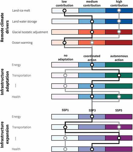
There are many ways in which climate change may unfold, how our society responds, and what our infrastructure requirements will be. As such, the future that manifests cannot be known with certainty or meaningfully described through the notion of probability alone (i.e., to say there is an x% chance that sea levels will have risen by y meters and adaptation will have happened in a given way, would be to grossly overstate our depth of understanding). The future can be explored through stories; stories that are conditioned by evidence from across physical, social, and political science. Given this context, a framework of reference is used that reflects a continuum of storylines within which any number of possible future system states can be considered (see, Figure 1). Alternative futures are illustrated by the storyline pathways 1 and n in Figure 1; where each storyline embeds three aspects of the future: (i) sea level rise; (ii) effort devoted to the adaptation of coastal infrastructure; and (iii) degree of expansion of coastal infrastructure (i.e., the development of new infrastructure for energy, telecommunication, and transport services among others). These alternative pathways represent the epistemic uncertainties around how the future will evolve (including the drivers of climate change and adaptation). Aleatoric uncertainty (related to the randomness in the climate and coastal flood response) is captured by imagining past storms to reoccur in the future to enable alternative realisations of each storyline. Use of this framework enables three important counterfactuals to emerge:

Figure 1. Storyline framework – Discrete storylines within a continuum of future system states. The grey and black line indicate possible storylines, which connect the choices in the remote climate drivers to sea level rise, the choices in infrastructure adaptation and the choices in infrastructure expansion. Individual choices can be made with regards to adaptation and expansion for different infrastructure types.

• Comparing the present and future risk given the same storm: How the recurrence of a past storm in the future may lead to different impacts.

• Comparing the risk in different storms in the same future: How different storms have different impacts given the same system state (present or future).

• Comparing the risk in the same storm in different futures: How the same storm may have different impacts in different future storylines.

Although conceptually there is no limit to the number of possible futures, there are practical limits. The notion of plausibility can be used to constrain the scope of future storylines without a significant loss of usability. For example, significant evidence exists on the plausible range of sea level rise and for much of this range, climate science provides a credible probabilistic description. There are constraining aspects of the future CI expansion. It is reasonable to assume that this responds to socioeconomic development with the associated uncertainty credibility described through the Shared Socioeconomic Pathways (SSPs). The ability to constrain the effort devoted to adaptation is harder to quantify but heuristic arguments readily enable plausible actions to be articulated. These arguments are used here (see, Section 2.2) to combine various forms of evidence to identity a small number of storylines that are then explored assuming three historic storms (Xynthia in 2010, Xaver in 2013 and in Emilia-Romagna in 2002). The limited number of storylines is driven by other practicalities (e.g., constraints on model runtime) and by the choice to provide a much more straightforward exploration of the future, both in terms of the interpretation of the model outcomes and socioeconomic implications.

2.1. Climate scenarios

The climate change aspect of the storyline framework considers the influence of four climate drivers that are significant in the context of sea level rise (Figure 1): (i) melting of land ice which includes Antarctica, Greenland and glaciers and ice caps around the world; (ii) land water storage; (iii) glacial isostatic adjustment; and (iv) thermal expansion and changes in ocean circulation. A change in storms could result in larger extreme sea levels and increased wave actions but there is still a large uncertainty about the potential magnitude of these effects (Bricheno & Wolf, 2018; Sterl et al., 2015); therefore, we only focus on mean sea level change in this study.

Some of the physical processes that will drive sea level rise along the European coast in the coming century are still highly uncertain (e.g., melting ice sheets, changes in ocean circulation). Therefore, it is useful to combine the usual probabilistic model (Le Bars, 2018) with a scenario-based approach. To do so, we either replace the probabilistic estimation of some contributors by a choice, or we explicitly choose one method to estimate the probabilities when another one, that would provide different results, would also have been possible. To build our sea level scenarios, the first element that we consider are the greenhouse gases (GHG) emission scenarios. The uncertainty for these GHG emission scenariosis not quantified in any probablistic way and requires one to make a choice from a selection of scenarios. . The second element that we consider is the future contribution of Antarctic dynamics. It is accepted to be one of the largest sources of uncertainty in global sea level projections (Bamber et al., 2019). We note here that the future amount of Greenland melt is also highly uncertain but since we are interested in future European sea level for which the fingerprint of Greenland is around 10% (Slangen et al., 2014), the regional uncertainty from Greenland is 10% of the global one. The third element that we use to define our scenarios is ocean dynamics as it is not very well constrained and yet it is important for European sea level projections (Vries et al., 2014).

These considerations are used to relate quantified evidence to each aspect of local sea level within the storyline framework (Table 1) and summarised below:

• ‘Low’ contribution is defined using the SSP1-2.6 scenario which results in around 1.8°C warming above preindustrial in 2100. The Antarctic dynamics is projected using a linear extrapolation of the observed discharge (Little et al., 2013). The ocean dynamics comes from GISS-E2-1-G, which is one of the few models for which this contribution is close to zero. To obtain a single value, we choose the 5^th percentile of the final probability distribution. This scenario can be used as a no regret policy; it is almost certain that sea levels will rise more than in this scenario so any adaptation measure for this level will be justified.

• Medium contribution uses the SSP2-4.5 emission scenario which results in 3.4°C warming in 2100. Antarctic dynamics is the same as for the low scenario, ocean dynamics is the ensemble mean and the final 50^th percentile of the probability distribution is chosen.

• High contribution presents a consensual ‘worst case’ because it does not include the controversial Marine Ice Cliff Instability (Bassis et al., 2021; DeConto & Pollard, 2016) that was shown to result in even faster sea level rise (Bars et al., 2017). It uses SSP5-8.5, the highest emission scenario that results in a warming of 5.6°C in 2100, and the latest linear response functions from ice sheet models that took part in the LARMIP-2 project (Levermann et al., 2020). The UKESM1-0-LL model is used for the ocean dynamics and the 95^th percentile of the final probability distribution is selected.

Table 1. Summary of the sea level scenario choices.

Scenario names	Emission scenario	Antarctic dynamics	Ocean dynamics	Percentile of final distribution
Low	SSP1-2.6	Little et al., 2013	GISS-E2-1-G	5th
Medium	SSP2-4.5	Little et al., 2013	Ensemble mean	50th
High	SSP5-8.5	Levermann et al., 2020	UKESM1-0-LL	95th

2.2. Coastal infrastructure choices

Future impacts due to coastal flooding will not only be driven by the dynamics of the earth system but also by socioeconomic developments. We make these socioeconomic developments explicit by building the components ‘coastal infrastructure expansion’ and ‘coastal infrastructure adaptation’ into the storylines (Figure 1). Infrastructure expansion can be interpreted as the investment and development of infrastructure within the coastal zone. An asset manager or regional authority may invest in new CI, without considering any form of adaptation. For example, the port of Zeebrugge may decide to build an entire new dock, with or without taking sea level rise into consideration. In other words, we can consider here how much infrastructure may be developed towards the future and how much a region may even ‘seize the opportunity’ due to climate change (i.e., port development in Norway due to new arctic sea trade). The boundaries of the adaptation and expansion aspects of the storyline framework used here are presented below.

2.2.1. Adaptation scenarios

The adaptation choices made by infrastructure owners will have a pronounced influence on the future coastal flood risk in Europe. Adaptation strategies can be implemented at various levels. At an individual asset-level, for example, one can raise critical aspects of the infrastructure (i.e., the power room or communication devices) to ensure they remain dry and functional during a flood (to a given flood level). Investment in flood protection dyke systems can provide regional protection to many CI assets. These different scales of adaptation are reflected within the boundaries of the adaptation scenarios considered here:

• No adaptation effort assumes no effort is developed towards adapting to climate change, and as the chance of flooding increases, so does the chance of the impact.

• Autonomous action assumes the individual CI owners act to improve on-site protection from flooding, that enables the CI to continue to function (without loss) given flood waters up to a depth of 0.5 metres. Dry-proofing is generally considered to be most effective for flood depths up to 1 meter (Han & Mozumder, 2021; May et al., 2014). Dry proofing, is, however, also considered to be a costly measure. As such, we apply a dry-proofing measure of ‘only’ 0.5 metres, comparable to the minimum of 2 ft (0.6 m) as suggested by Defra and FEMA (Aerts, 2018; May et al., 2014). This means that no damage will occur at inundation depths lower than this threshold.

• Coordinated action representing collective action to deliver a reduction in risk.(i.e. recognising protection relies on all dykes protecting an area to be improved). It is assumed here that the existing flood defence system (e.g., dyke) in place is maintained to the standard it was originally designed for. More specifically, a dyke that is designed to withstand a flood with a probability of 1/100, will also withstand a probability of a flood with a probability of 1/100 in the future (which may have become more severe relative to the present day).

2.2.2. Coastal expansion scenarios

Thus far, no information is available on the spatial distribution of CI in a future world, while such input is essential for CI risk assessments in which future socioeconomic development is accounted for. We therefore develop a set of future states of coastal infrastructure expansion embedded in the SSPs, as a set of socioeconomic counterfactual scenarios. SSPs are defined as ‘reference pathways describing plausible alternative trends in the evolution of society and ecosystems over a century timescale, in the absence of climate change or climate policies’ (O’Neill et al., 2014). Merkens et al. (2016) developed population distribution projections that are built upon these SSPs, which were enriched with narratives based on a series of coastal migration drivers to account for subnational population dynamics (e.g., coastward-migration).

To link the SSPs to coastal infrastructure expansion, we assume that infrastructure expansion is a function of population growth (which is also considered to be an important driver of trends in GDP). For the representation of CI in the counterfactual scenarios of coastal expansion, we adapt the Critical Infrastructure Spatial Index (CISI). The CISI is a composite index expressing the spatial density of CI (Nirandjan et al., 2022). The future infrastructure density is estimated for three pathways assuming that the change in the amount of infrastructure is proportional to the change in population (i.e. we assume that infrastructure density is mostly driven by local economic activity). The three future alternatives for infrastructure expansion are explained below:

• SSP1 (Green Coast) represents the world’s shift towards a sustainable pathway, which results in well-managed coastal zones that are characterized by compact cities which are regulated by environmental policies.

• SSP3 (Troubled Waters) represents a pathway in which the coastal zone management follows national and regional security constraints, but socio-economic development is poorly managed leading to a converging population distribution over time amongst coastal and inland areas.

• SSP5 (Coast Rush) represents a highly globalized world promoting socio-economic development in the coastal zone leading to high population growth that results in large cities with urban sprawl.

3. Methods: Storyline quantification

3.1. Extreme sea levels

Extreme sea level conditions for the storms, now and in the future, are modelled using the Global Tide and Surge Model v3.0 (GTSMv3.0). GTSMv3.0 is a depth-averaged hydrodynamic model with global coverage that dynamically simulates tides and storm surges. The model has global coverage and is forced by the tide-generating forces and external forcing fields (e.g., winds, surface pressure). The uniform bottom friction coefficient and internal wave drag coefficient have been tuned to match observed total rates of energy dissipation. For surges, the relation by Charnock (1955) to model the wind stress at the ocean surface is used, and the drag coefficient has also been tuned during the calibration process. Here, we use a GTSM reanalysis dataset that was computed by forcing the model with the ERA5 reanalysis. This dataset provides information on real historical water-levels between 1979 and 2017 (Muis et al., 2016).

GTSM is a free-running model without assimilation of observed tides or surges that constrain the solution. It uses the unstructured model Delft3D-FM (Kernkamp et al., 2011) to employ a flexible distribution of resolution, which results in high local accuracy at a lower computational cost. It has a 1.25 km coastal resolution in Europe. The resolution decreases from the coast to the deep ocean to a maximum of 25 km. Increased resolution is added in the deep ocean with steep topography areas to enable the dissipation of barotropic energy through generation of internal tides. The bathymetry used consists of a combination of EMODnet high-resolution (250 m) data corrected for LAT-MSL differences and General Bathymetric Chart of the Ocean 2014 (GEBCO, 2014) with a 30 arc second resolution (Weatherall et al., 2015).

Sea level change along the European coast for the medium contribution in 2120–2125 is shown in Figure 2 (left panel). The spatial differences in sea level rise in this map are mostly due to ocean dynamic sea level and to the glacial isostatic adjustment. Other processes are fairly spatially homogeneous along the European coast. Time series of sea level for the three scenarios in Northern Germany up to 2125 are shown in Figure 2 (right panel). The sea level change used as a forcing to the flood model for the three storms and the three scenarios is given in Table 2. For each event, sea level rise is considered by changing the background sea level onto which the extreme sea level resulting from the storm surge modelled by GTSM3.0 is added.

Figure 2. Map of sea level change in 2120–2125 compared to 1986–2005 for the medium scenario (left). Time series of the three sea level scenarios in the Northern German coast for the Xaver storm.

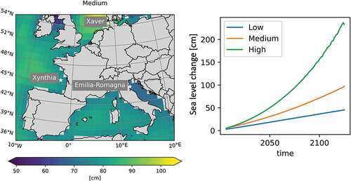
Table 2. Sea level rise in cm between the date of the storms and 2120 for the three climate scenarios.

Storm	Period	Low	Medium	High
Xynthia	2010–2120	25	71	204
Xaver	2013–2120	39	82	211
Emilia-Romagna	2002–2120	24	64	190

3.2. Coastal inundation modelling

To estimate coastal flood maps for our storylines, we use the ANUGA model, developed by the Australian National University (ANU) in collaboration with Geoscience Australia (GA). ANUGA is a 2D-Hydrodynamic model capable of simulating the free surface elevation of water flow over land areas (Roberts et al., 2015). The fluid dynamics in ANUGA are based on a finite-volume method for solving the shallow water wave equations, being based on continuity and simplified momentum equations (Zoppou & Roberts, 1999). ANUGA uses an irregular triangular grid, thus allowing for the use of coarser or finer grids over specific areas and potentially providing more accurate spatial representation of the 2D domain. For each triangular element and time step, the model computes the (i) water surface level, (ii) bed elevation (and depth) and (iii) horizontal (x and y) momentum. ‬‬‬‬‬‬‬‬‬‬‬‬‬‬‬‬‬‬‬‬‬‬‬‬‬‬‬‬‬‬‬‬‬‬‬‬‬‬‬‬‬‬‬‬‬‬‬‬‬‬‬‬‬‬‬‬‬‬‬‬‬‬‬‬‬‬‬

The time-independent parameters of the ANUGA model are the bed elevation and the bed friction (Manning friction coefficient, a forcing term), while the initial conditions of the model are the water stage (height of water surface) and the x- and y-momentum. We use a high-resolution Digital Elevation Model (DEM; Kulp & Strauss, 2018) and the European Marine Observation and Data Network (EMODnet) bathymetry data (Thierry et al., 2019) to characterise the bed elevation in the ANUGA domain. The base DEM used is the high-accuracy CoastalDEM (Kulp & Strauss, 2018) for coastal areas, at 90 m resolution. Coastal defences such as dykes and sea walls are extracted from OpenStreetMap (OSM; Haklay & Weber, 2008).

Every triangular element in ANUGA is initialised according to the water level and x- and y-momentum in GTSM at the beginning of an event (e.g., storm Xaver). The boundary conditions are prescribed with the GTSM water level data for the duration of the simulation. Momentum data is manually calibrated to best emulate the storm surge wave propagation inside the model’s domain. For instance, if an event is moving south-west to north-east, the momentum is specified so that the water flow entering the domain accounts for these dynamics. This setup allows for the numerical simulation of the propagation of flood waves and inland inundation.

ANUGA can account for the presence of coastal defence structures. In particular, the dynamics of coastal defence structures can be simulated by modifying the bed elevation. This is particularly useful when simulating the activation of mobile gate systems (e.g., Porte Vinciane, a mobile gate system in Cesenatico, Italy) or dam/levee breaks (e.g., the sea wall in the coastal town of L’Aiguillon-sur-Mer destroyed by storm Xynthia in Western France). By considering not only the presence as well as the dynamics of coastal flood defences, ANUGA can simulate the temporal and spatial evolution of the flood extent, water depth and momentum of a particular flood event. The results for the application of ANUGA for the storms Xynthia, Xaver, and along the Emilia-Romagna coast are shown in Appendix A. It is important to highlight that the coastal inundation modelling under the different climate scenarios considers the large-scale dynamics of the assessed storms to be constant (e.g., intensity, duration, landfall), while the inundation dynamics resulting from the combination of sea level and storm-surge are recomputed for each climate scenario and for each case study using the hydrodynamic model ANUGA.

3.3. Critical infrastructure damage assessment

For this analysis, we represent the CI network by seven overarching CI systems that are generally discussed in the literature: energy, transportation, telecommunication, water, waste, education, and health (Nirandjan et al., 2022). We use OSM to extract relevant infrastructure types applying 96 active OSM tags representing 41 infrastructure types that are categorized under the seven overarching CI systems (see Appendix B). To assess the direct damages to infrastructure assets, we follow a traditional physical damage assessment approach (Koks et al., 2019b; Winsemius et al., 2016), in which we combine the geospatial information of the infrastructure assets with flood hazard data on inundation levels and extent, by using state-of-the-art vulnerability information as described below.

The potential direct damage to CI is estimated using vulnerability functions (also known as depth-damage or stage-damage curves). They show the relationship between an intensity measure of the flood hazard and the potential damage to a specific infrastructure type. Potential damage can either be expressed in absolute values or as a percent (i.e., 0–100% damage). We apply vulnerability curves that are expressed in the form of the potential percent damage as a function of water depth in our analysis. The damage values, based on construction costs, are used to estimate the potential damage in euros for a specific asset (reference year 2015) that experiences a certain level of inundation. Vulnerability functions, however, are not available for all infrastructure types. In such cases, we assume that we can apply vulnerability functions of infrastructure that have the same characteristics (e.g., construction material, diameter/height ratio, and type of service). In case of infrastructure types lacking damage data that can be used directly for risk assessments, we use construction costs derived from literature and assume that the costs for reconstruction are 60% of the original construction costs (e.g., Huizinga et al., 2017). See Appendix C for a detailed overview of the references for the vulnerability functions, damage data, and assumptions.

As the CI dataset consists of points, polygon, and lines, three approaches to process these datatypes are developed accordingly (Koks et al., 2021). For all datatypes, we apply the same principle, whereby we use the geospatial location of the infrastructure asset to detect whether the asset is in an inundated area. The inundation depths for each location are combined with asset-level vulnerability information to calculate the damage. To process the damage for inundated point features, we extract the inundation value that directly overlaps with the asset under consideration. This specific inundation level is then combined with the available vulnerability information for that specific asset-type to estimate the total damage.

This is, however, different for line and polygon features as one asset can be present in multiple inundation cells. For inundated line features (e.g., primary road), we therefore calculate the length (in meters) of a linear asset that overlaps with each unique inundation cell (e.g., 10 m overlap with an inundation of 40 cm, 8 m overlap with an inundation of 60 cm, etc). The exposed length is then combined with the inundation level of the given inundation cell through the vulnerability curve that holds potential damages per exposed meter. For polygon features (e.g., hospital), we calculate the inundated area (in square meters) per inundation cell that overlaps with the polygon asset. Subsequently, the exposed area is then combined with the inundation level of the given inundation cell and vulnerability information that holds potential damages per (1) exposed square meter or (2) per facility for a given infrastructure type. In the latter case, we disaggregate the maximum damage that may occur to a complete asset (e.g., power plant) to the potential maximum damage that may occur per square meter.

3.4. Critical infrastructure adaptation and expansion

To estimate the future potential direct damage, we implement a future alternative of the climatological and socio-economic setting. As extensively explained in Section 2.1 and Section 2.2, this means that we estimate the damage for each storyline which is a combination of one of the three future climate scenarios (Section 2.1), one of the three future adaptation scenarios (Section 2.2.1) and one of the three future socioeconomic expansion scenarios (Section 2.2.2). Future climate change will influence the height of the direct damage through a change in inundation depth and extent. To assess how adaptation may influence future damages, we analyse the effect of maintaining the strength of a dyke (i.e., maintain the same design standard as the current situation) and the effect of dry proofing. The first adaptation option is included through ensuring that during the inundation simulation modelling, the coastal defences do not collapse. The second adaptation option is included within the damage assessment through setting all potential damage to zero for all inundation up to 0.5 meters (please refer to Section 2.2.1 for a justification of this assumption). The third adaptation is a ‘do-nothing’ scenario. Future coastal expansion is, within our analysis, driven by future population expansion. Due to a lack of research on the potential future development of infrastructure, it is assumed that population expansion can be considered as a proxy for infrastructure demand (please refer to Section 2.2.2 for a further elaboration on the chosen scenarios). In practical terms, it means we overlay each infrastructure asset with the changes in population density for each of the three ‘coastal expansion’ scenarios and correct the estimated damage for that particular asset accordingly.

4. Storyline foundation: the three events

4.1. Storm Xynthia

Storm Xynthia was a severe windstorm which crossed Western Europe between 27 February and 1 March 2010, causing casualties and major damage in multiple countries. The storm started as a depression over the Atlantic Ocean and subsequently developed under supportive climatic conditions into a heavy storm. Storm Xynthia made landfall along the coast of France during the night of 28 February, continued its path in a northeast direction, and eventually faded out over the southern Baltic Sea within a time span of 24 hours. The storm led to coastal floods, with the coastal areas of the Vendée and Charente-Maritime in France particularly hard-hit. Intense wind gusts were measured along the Western Coast of France. Wind gusts of approximately 160 km/h were detected at the island Île de Ré and the department Deux-Sévres, and 130 km/h at stations in the coastal towns La Rochelle and Les Sables-d’Olonne. The combination of storm surge, a high tide and wave setup resulted in high water levels, with the highest water level of 4.5 metres NGF (General Levelling of France) measured at La Rochelle (Kolen et al., 2010).

An area of more than 50,000 ha was flooded causing 47 fatalities in Vendée and Charente-Maritime (Kolen et al., 2013). The storm resulted in widespread material damage to houses, (agricultural) businesses, and infrastructure. Major power failures left 1 million households without power services (that lasted at least 12 hours in some areas); boats, pontoons and landings in flooded harbours were destroyed; and the coastal railway between La Rochelle and Rochefort was shut down for several weeks. Multiple flood defences failed, including seven dyke locations in Gironde (Kolen et al., 2013), while other flood defences along the coast were damaged due to overtopping and erosion processes (Kolen et al., 2010). The damage in France caused by the storm was estimated to be around 1.5 billion euros, of which 700 million has been attributed to flooding (Chauveau et al., 2017).

4.2. Storm Xaver

Storm Xaver formed as a low-pressure system from a warm front wave over the North Atlantic south of Greenland on 4 December 2013, which rapidly evolved into a winter storm (Deutschländer et al., 2013). Xaver crossed Northern Europe on 5 and 6 December 2013, with high wind speeds (e.g., 160 km/h in Germany; Deutschländer et al., 2013). Compared to the infamous and severe 1953 storm when around 2200 people lost their lives across the North Sea region, storm Xaver had a smaller surge but coincided with a larger astronomical tide. This coincidence of astronomical and meteorological drivers results in a much greater length of coastline experiencing extreme high-water levels (Wadey et al., 2015). Flood barriers in different countries had closed their gates to protect areas behind the barriers from flooding. For example, the Netherlands closed the Eastern Scheldt storm surge barrier, and flood gates to protect Hamburg were activated (Spencer et al., 2015). On 6 December 2013, the Thames Barrier experienced the highest water levels since its completion in 1982 and was kept closed for two consecutive days (Wadey et al., 2015).

The flood defences, developments in forecasting, and improved risk management systems (e.g., warning systems and evacuation plans) prevented the high death toll that was experienced during a similar storm surge in 1953 (RMS, 2014; Spencer et al., 2015). However, storm Xaver was one of the costliest storms to hit Europe: insured losses are estimated to be in the range of 1.4–1.9 billion euros (Wadey et al., 2015), and economic losses are likely to be even higher (Rucińska, 2019). It should be noted, however, that most of these insured losses can be attributed to wind damages. Record-breaking water levels were measured along large parts of the German Bight coastline on 6 December 2013 (Dangendorf et al., 2016). The port city of Hamburg measured a storm surge of 6.09 m above mean sea level, which led to flooding in only some parts of the city due to the effectiveness of the flood protection structures (RMS, 2014). Large-scale power outages (mostly wind-triggered) occurred in the UK, Ireland, Poland, southern Sweden, and areas of Northern Germany (Kettle, 2020). Port operations were interrupted, offshore wind farms were shut down, and flight and rail services suspended.

4.3. Storm surge in Emilia-Romagna

In 2002, a succession of storms resulted in a series of extreme sea level events between November 14 and November 19 along the North Adriatic coast of Italy. The coastal area of the Emilia-Romagna Region was particularly hard hit, with significant wave heights of about 4.70 m (in a North-Northeast direction and average wave period of 7.1 seconds) registered close to the municipalities of Rimini and Cesenatico. Coastal flooding occurred in Rimini, Cesenatico, and Marina di Ravenna, with erosion occurring along the coast of Rimini and to the south of the Po Delta. The worst coastal flooding episode was registered at the tide gauge of Ancona on the 15^th of 8 November 2002:30 AM local time with significant wave heights of 5.20 m, wave periods of 10.5s and wave direction of 122° North (Perini et al., 2011).

The Rimini coastline was severely damaged by the event with damages reported to coastal defence structures and buildings and 12,000 tons of material accumulated along the coastline. Multiple municipalities and locations requested that a state of emergency was to be declared. The ports of Riccione and Bellaria-Igea Marina required emergency dredging. Approximately one million euros were allocated for interventions such as cleaning and nourishment of critical points along the coast of Emilia-Romagna as a result of the events (Perini et al., 2011).

5. Results

5.1. Xynthia

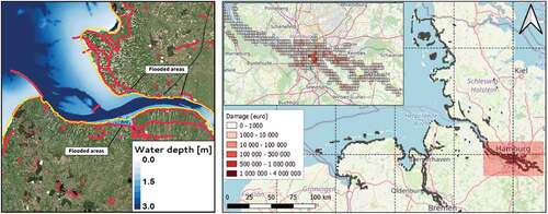
The storm surge from Xynthia was mainly driven by a wind-forced Ekman setup (Bertin et al. 2012) and the impact of the storm on sea level was strongly increased by coinciding with a spring tide (Koks et al., 2021). For Storm Xynthia, most of the recorded damages were caused by the rupture of seawalls and by the subsequent flooding (see, Section 4.1). These effects are represented in our simulated inundation modelling by considering the collapse of a seawall near the coastal town of L’Aiguillon-sur-Mer (left panel, Figure 3). In-line with observations, the storm peak is simulated near the city of La Rochelle (located in the bottom of the left panel in Figure 3).

Figure 3. Left panel: Coastline section where storm Xynthia made landfall. In red, the area where the seawall collapse is simulated. The yellow line indicates the coastline. Flooded areas are indicated in shades of blue, according to the water depth. Right panel: The spatial distribution of locations that suffer damages to CI along the coastline of Western France.

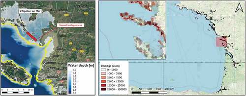
Damages to infrastructure due to storm Xynthia are widespread along the coastline of Western France within our simulation of the historic event. Figure 3 shows the spatial distribution of damaged infrastructure, whereby further detail of the estimated damages is given to La Rochelle and surroundings that are particularly hard-hit. The total estimated damage to critical infrastructure due to flooding in the coastal areas of western France is approximately 10 million euros, based on our inundation modelling. The CI system transportation has, with a damage of 9.1 million euros, the highest contribution to the total damages (Appendix D). The remainder of damages is due to damaged waste facilities (~8%), education facilities (1.7%), followed by health care (0.6%) and the energy system (<0.01%). The water and telecommunication systems remain undamaged in our analysis.

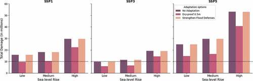
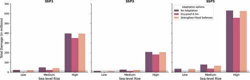
Figure 4 presents the results for all future counterfactuals, and the historic event indicated by the dotted horizontal line. Interestingly, the modelling results indicate that the lowest future damage is expected through a storyline in which the coastline of France follows the SSP3 (‘Troubled Waters’) infrastructure expansion storyline path, due to the relatively limited coastal development and even reductions in some places. The most extreme scenario (expansion driven by the boundary conditions of SSP5 and high sea level rise) results in almost a fivefold increase in damage relative to the historic event. In the case of storm Xynthia, further strengthening of the current flood defences (i.e. seawalls are reinforced and thus not subject to collapse, see, Section 2.2.1) results in relative minor reductions in damages, whereas dry-proofing individual CI assets up to 0.5 m (i.e. autonomous action, see, Section 2.2.1) can result in a roughly 30% decrease in total damages.

Figure 4. Total coastal flood damage estimates for storm Xynthia under three socioeconomic infrastructure expansion scenarios (the three panels), three climate change scenarios (the grouped bars) and three adaptation measures (the colours). The dotted line indicates the simulated damage for the reference event.

When further disentangling the storyline results for each CI system, we find some interesting differences between the various systems affected. While the damage share of the transportation system remains similar and the highest (~90% of the total damages), the share of the energy system within the total damage for the ‘no adaptation situation’ increases from ~0% towards 3–5%, depending on the SSP scenario. The share of the waste sector, on the other hand, reduces from ~8% to around 4%. The largest differences between SSP3 (the overall lowest estimates) and SSP5 (The overall highest estimates) are found for the waste (~230% higher within SSP5) and energy system (~204% higher within SSP5). Also, towards the future, telecommunication and water infrastructure remain undamaged in our analysis. With respect to the different adaptation measures, we find some notable differences between the effect of dry proofing between the CI systems. For both low and medium sea level rise, healthcare and education experience the largest reductions (>70%), followed by transportation (~40%). For high sea level rise, however, the overall reduction is much smaller compared to the no adaptation scenario (e.g., only a ~ 30% reduction for the education system). This indicates that under high sea level rise, much more assets experience larger flood depths. Both energy and waste assets only experience a reduction between 1% and 5% when dry proofing.

5.2. Xaver

Sea level at the German coast reached a record high during storm Xaver. The peak was the result of a combination of high surge, mean sea level and high tide coinciding in time. The inundation process is simulated at around the maximum water level height of the event, accounting for the propagation of the storm surge wave in direction to the coastline and is thus started on 6 December 2013 and lasting for 16 hours. The model accounts for a temporal resolution as low as 1 arcsecond, while information regarding the dynamics of the event is saved to the output file every simulated 5 minutes, thus allowing for identifying the wetting and drying of flooded areas. Coastal defence structures are accounted for as vertical barriers in the terrain, and, differently from the case of storm Xynthia, no seawall collapse is simulated, while a strengthening of the seawalls (raise of 1 m) against coastal flood events is simulated under the adaptation scenario.

Most of the potential damages were avoided by the presence of coastal defence structures. At present, the height of primary sea dykes in the Wadden Sea region ranges between 6 and 9.5 m above mean sea level (CPSL, 2005). In the absence of detailed data characterizing the specific height of each individual coastal defence segment, we assume a mean height of 6.5 m for the considered coastal defence structures (Left Panel, Figure 5). Consistent with observations and the data from GTSM, the storm peak is simulated to take place near the city of Cuxhaven. Infrastructure damages due to storm Xaver are widespread along the coastline of Northern Germany, resulting in a total estimated damage to CI of approximately 1.7 million euros (Appendix B). The right panel of Figure 5 shows the spatial distribution of damaged infrastructure within our simulation of the historic event, with further detail of the aggregated damages zoomed in on Hamburg. The highest estimated damage is to the CI system transportation (65.8%), followed by waste (21.4%), education (9.1%), and energy (1.8%). Although multiple telecommunication assets are exposed to flooding induced by storm Xaver, they are not damaged in our model simulation.

Figure 5. Left panel: Coastline section where storm Xaver made landfall. In red, the area where the seawall is present in the simulation. The yellow line indicates the coastline. Flooded areas are indicated in shades of blue, according to the water depth. Right panel: The spatial distribution of locations that suffer damages to CI along the coastline of Germany.

Figure 6 presents the results for all counterfactuals for storm Xaver, including the total damage for the historical event. The results show approximately 22 million euros of direct damage in the counterfactual that has large infrastructure expansion (SSP5) in the future, no adaptation and high sea level rise. This is roughly 12 times larger relative to the historic event. The strengthening flood defences provide the largest overall reduction in damages. Dry-proofing assets up to 0.5 m again also substantially reduces the losses by a factor 3 to 4 depending on the counterfactual.

Figure 6. Total coastal flood damage estimates for storm Xaver under three socioeconomic infrastructure expansion scenarios (the three panels), three climate change scenarios (the grouped bars) and three adaptation measures (the colours). The dotted line represents the simulated historic event.

For CI systems individually, we find that the share of the transportation system within the total damage estimates increases within the ‘no adaptation’ scenario towards ~83%. Already under low sea level rise, the damage to transport infrastructure may increase with 346% under SSP3, and up to 1,100% under SSP5. The education system experiences the second largest increases, ranging from 189% (SSP3) to 695% (SSP5). The waste system experiences the smallest relative changes towards the future, and its relative share in the total damages reduces towards ~9%. The share of the other systems remain more or less the same. Both dry-proofing and strengthening flood defences can cause a substantial reduction in damages. For low and medium sea level rise, dry proofing fully mitigates the damages for healthcare assets. The damage reduction as a result of strengthening flood defences is for most CI systems above 70%. Only the waste system experiences a reduction of only ~50% for medium and high sea level rise. This may indicate that waste assets are currently built in locations that may not be sufficiently protected against higher inundation levels due to sea level rise.

5.3. Emilia-Romagna

Sea level at the Italian coast along the Emilia-Romagna Region were close to record high during a series of storm surge events in November 2002 (Koks et al., 2021). The peak was the result of a combination of high surge, high tide, and wave height coinciding in time. We incorporate the presence and height of coastal flood defences by relying on LiDAR data available along the coastal zone of Italy (Geoportale Nazionale, 2015). Figure 7 displays the water level distribution along the coastline of the Emilia-Romagna Region during the maximum simulated water levels. As observed, coastal flooding is simulated near the cities of Rimini, Cesenatico, and Cervia.

Figure 7. Left panel: The storm surge event of 15 November 2002, as simulated by ANUGA when the storm surge hits the city of Rimini. In red, the area where the coastal defence project called ‘Parco del Mare’ is located. The yellow line indicates the coastline. Flooded areas are indicated in shades of blue, according to the water depth. Right panel: The spatial distribution of locations that suffer damages to CI along the coastline of the Emilia-Romagna region.

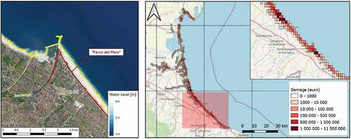
Coastal flooding in the Emilia-Romagna Region results in damaged infrastructure along the entire coastline, particularly in the coastal towns of Ravenna, Cervia, Cesenatico and Rimini. The right panel in Figure 7 presents the spatial distribution of damaged infrastructure within our simulation for the historic event. CI situated along the coast in the Emilia-Romagna region exposed to the flooding resulted in a total estimated damage of 12.5 million euros. The estimated damage to the waste facilities amounts 8.1 million euros and has therefore the highest contribution (65.3%) to the overall damage to critical infrastructure. The transportation system also suffers a considerably high damage, namely 2.1 million euros (16.9% of the total damage). This is then followed by the CI system education (10.8%), healthcare (5.6%) and energy (1.4%). The road network accounts for 85% of the total damages within the transportation system, while the remainder is due to damages to multiple parts of the railway network and one small-scale aerodrome in Ravenna. The simulated damages within the energy system are predominantly caused by a flooded power plant in the industrial area of Ravenna, and a substation in Cervia.

Figure 8 shows the results for the 27 counterfactuals for the storm surge event in Emilia Romagna. The results clearly indicate that sea level rise, and in particular the high sea level rise is the dominant driver for increased damages to infrastructure assets. The low sea level rise scenario (~24 cm increase) results in practically the same flood damage relative to the historic event. Dry proofing can fully offset the damages for the storylines in which we have selected low sea level rise. Depending on the infrastructure expansion, damages increase by a factor 16 to 50 for the high sea level rise storylines. Dry-proofing infrastructure assets up to 0.5 m shows results in a larger decrease in damages, relative to maintaining the design standards of the flood defences.

Figure 8. Total coastal flood damage estimates for the storm surge event in Emilia Romagna under three socioeconomic infrastructure expansion scenarios (the three panels), three climate change scenarios (the grouped bars) and three adaptation measures (the colours). The dotted line represents the simulated historic event.

Under a high sea level rise scenario, we see very large increases across all CI systems. Whereas the waste sector accommodated ~65% of the damages for our damage assessment of the historic event, it only accounts for ~18% under high sea level rise and all future SSPs. This is despite the fact that the damages of the waste sector still increase between 340% (SSP3) and 1,315% (SSP5). The energy system experiences the largest increase, of up to 80,000% under SSP5 (i.e., almost no damage to the energy system occurred in the historic reference). Across all SSPs, the energy system now accounts for ~22% of the damages. The second largest increases can be found in the transportation system, ranging from a 3,600% (SSP3) to 10,500% (SSP5). This is closely followed by the healthcare and education system. Under low and medium sea level rise, dry proofing can fully mitigate the damage to the waste system. On average, dry-proofing assets reduces the damage across all CI systems by around 94% for low sea level rise. Under medium sea level rise, this mitigation effect reduces to an average of 66%, and to only 10% for high sea level rise. We observe some interesting dynamics across the different CI systems. The education system experiences a very large drop in the mitigation effect of dry proofing between low and medium sea level rise (94% to 16%), while the energy system only experiences this drop between medium and high sea level rise (83% to 1%). This indicates that energy system assets still experience relative low water depths under medium sea level rise, whereas multiple educational assets are already substantially flooded (reducing the effect of dry proofing up to 0.5 m of inundation).

6. Discussion

The use of storm-event-based storylines within our presented framework, in which we consider how a past storm may impact a future world if it were to reoccur, helps to bring the future to life. Placing historical storm events in the context of such a framework reinforces the notion that there are multiple futures that are plausible whilst maintaining clarity. In particular when dealing with ‘the future’, whether this is sea level rise or future infrastructure investments, one generally has to deal with the presence of deep uncertainty (Kalra et al., 2014). When one translates global processes, such as climate change, to the impacts on a local level, large uncertainties are inevitable. While the quantification of all these uncertainties may be desired, it is often simply infeasible to do so. Either because some of the uncertainties are simply not known, or the parameter space is simply too large to realistically model this. Storylines allow this uncertainty to be explored in a recognizable and physically plausible way (Shepherd et al., 2018).

Our presented framework enables specific futures to be constructed (through evidence-guided expert judgment) that illustrate the future space that has the greatest resonance to specific historic events. For example, Xynthia, Xaver and Emilia-Romagna are recognised storm events, experienced by CI providers and local authorities. By exploring how the future changes, these storm-events enable CI providers and local authorities to access the scale of future change in an accessible form. For example, in the case of storm Xynthia, focusing solely on the strengthening of existing flood defences is shown to yield only minor reductions in damages should the storm occur again, whereas focusing on local resilience though dry-proofing individual infrastructure assets would achieve a 30% decrease in total damages. This connected narrative provides a clarity that may be difficult to achieve through a conventional probability risk assessment alone (Hazeleger et al., 2015).

By linking the storyline framework to past events, the focus is on the ‘credible and plausible’ rather than ‘probable and probability’. The retelling of the storm event stories illustrates their ability to explore future conditions and impacts without complex communication of a real-world probabilistic analysis (i.e., one that may include climate, flood, socio-economic and adaptation consideration). Overall, our approach helps to improve scientific understanding, but forces a distillation of the science into a narrative (Sillmann et al., 2021). This requires the storyteller to marshal often complex information into accessible narratives, suitable for the local actors at stake and tailored to the specific case of interest (Hazeleger et al., 2015). This process forces an open dialogue with the evidence that help to identify gaps in knowledge as well as supports policy understanding. This type of analysis and communication can provide a powerful voice within national debates. In England for example, the use of storyline evidence to illustrate the need to realign the shoreline under different climate futures, is gathering increasing attention as part of the Shoreline Management Planning (SMP) process (Sayers et al., 2022b). SMPs emerged in the mid-1990s to support a strategic approach to the management of coastal erosion and flood risks but there is often a difficulty in illustrating the changing risks in a meaningful way, and a lack of clarity as to how this transition will be made where this is required. Although the time horizons often appear long into the future, transformative change takes time. Storylines have a role ensuring communities and CI providers are meaningfully engaged in the decision process; a prerequisite for action (e.g., DEFRA, 2015).

Many countries across Europe, and further afield, have a long-term ambition to create a nation more resilient to future coastal flooding. The UK Government policy statement on flooding and coastal erosion (HM Government, 2020) articulates this ambition: ‘To create a nation more resilient to future flood and coastal erosion risk. In doing so, reduce the risk of harm to people, the environment, and the economy. We will be better protected to reduce the likelihood of flooding and coastal erosion. We will be better prepared to reduce the impacts when flooding does happen.’ Regardless of emission controls, sea levels are set to rise and adaptation will be central to achieving societal resilience to coastal flooding. Assuming a 2°C rise in GMST by the end of the century (compared to pre-industrial times), and limited adaptation (with present-day protection standards reducing in all but major urban conurbations) the number of residential properties exposed to a significant chance of coastal flooding could increase six-fold by 2080s and tenfold given a 4°C rise within England (Sayers et al., 2022a). While such aggregated numbers provide useful context, they only provide a limited insight into how this risk may be different given different future mitigation and adaptation choices and for individual sectors and infrastructure providers. The storyline framework developed bridges this gap between aggregated statements of changing risk and how future impacts may change for an individual sector or CI provider, and the actions they can take to reduce their risk. The framework set out here links the global drivers of climate and the influences of socio-economic development to localized action, including adaptation decisions made by regional authorities (e.g., the raising of dykes) and the actions of individual CI owners.

As we have applied only two adaptation strategies (dry-proofing and strengthening flood defences) within our analysis, we acknowledge that this is a limited vision towards climate adaptation. To enhance transformational change at the shoreline (including through relocation, Sayers et al., 2022b) and to succesfully reduce future risk, a broad portfolio of adaptation options is required. This may range from the use of nature-based solutions to attenuate incident waves conditions and to maintain beach levels (Aerts, 2018; Reguero et al., 2018), to catchment and planning responses(e.g., Evans et al., 2004; Sayers et al., 2013). Although not explicitly considered here, the framework of analysis presented does not constrain their inclusion. The framework allows for assessing any type of adaptation strategy, including adaptation measures more rooted into nature-based solutions and portfolio-based responses.

Yet, several opportunities exist to develop the approach to better support the policy decision-making processes. In particular, the approach for the development of the infrastructure expansion counterfactual can be advanced by: (1) extending the number of variables that drive infrastructure expansion (e.g., GDP) rather than only driven by population change; and (2) explicitly considering the local context through more extensive stakeholder engagement. With the latter we refer to, currently enforced or future regulations (e.g., building restrictions in specific zones), and ongoing or to be implemented infrastructure projects (e.g., new highways for increased connectivity) that affect the spatial distribution and expansion of infrastructure, and thus the future coastal risk. Moreover, while we have primarily focused on asset-level damages to infrastructure, disruption of economic activities as a result of infrastructure failure can substantial increase the total impacts. Not only because the impact footprint may become much larger than only the flooded area, but also due to on-going disruptions while assets and networks are still being reconstructed (Koks et al., 2019a).

7. Conclusion

In this study, we have presented a storyline framework to establish a consistent set of storylines to assess the impact of future climatic and socioeconomic conditions on coastal flooding impacts along the European coastline. We have illustrated the framework through multiple historic events. The framework allows for the combination of well-established quantitative methods for sea level rise, coastal inundation modelling and infrastructure damage assessments into a flexible integrated modelling approach that can be easily applied within a regional and local context. The approach explicitly does not set a specific time dimension to the model assumptions and choices. It can be used to estimate the potential socioeconomic impacts through setting plausible and coherent boundary conditions to create a realistic narrative for a potential future situation.

We have applied this approach for three historic storm events: storm Xaver (northern-German coastline), storm Xynthia (French coastline) and a storm surge event along the coast of Emilia Romagna (Italy). Future sea level rise was categorized into three ‘levels’, ranging from low sea level rise (25–40 cm, depending on the storm event) up to high sea level rise (~2 m). Expansion of infrastructure was exemplified through three different scenarios, ranging from low to high coastal development, driven by future population projections. Finally, adaptation was exemplified through two different adaptation options: asset-level dry proofing (autonomous action) and maintaining the design standards of flood defences (coordinated action).

The drivers for future changes vary between the three historic storm events. For Storm Xaver, we find that the socioeconomic boundary conditions (i.e., infrastructure expansion) are the most important driver for future damage increases, whereas for Storm Xynthia and the storm surge event along the coast of Emilia Romagna, sea level rise is a more dominant driver. Yet, all events show a substantial range in potential damages between their different storylines, indicating that identifying such a range of potential futures (or counterfactuals) is essential to support the policy-making process to move towards a more climate resilient future. Our approach helps to improve scientific understanding, through forcing a distillation of the science into a narrative to support the process towards a climate resilient society.

The utility of the framework is illustrated in the context of coastal flood risk in Europe. The framework however is more broadly applicable. Although the underlying models are context specific (the storms, the physical processes and damage functions) the framework of storyline ‘thinking’ (and the concept of a continuum of futures and use of selected storyline pathways) is readily transferable to other locations and settings. Furthermore, while the damage assessment in this study has focused on asset-level impacts, future work is recommended to further include an assessment of the wider economic impacts due to disrupted infrastructure networks and the failure of their services.

Disclosure statement

The Coalition for Disaster Resilient Infrastructure (CDRI) reviewed the anonymised abstract of the article, but had no role in the peer review process nor the final editorial decision.

Additional information

Funding

The Article Publishing Charge (APC) for this article is funded by the Coalition for Disaster Resilient Infrastructure (CDRI). This research was carried out and funded as part of the EU Horizon-2020 project RECEIPT (Grant Agreement No: 820712). Elco Koks was further supported by the Netherlands Organisation for Scientific Research (NWO; grant no. VI.Veni.194.033).

Notes on contributors

Elco E. Koks

Elco E. Koks is an Assistant Professor within the department of Water and Climate Risk at the Institute for Environmental Studies (IVM). His research combines knowledge from disaster impact modelling, critical infrastructure, network analysis and macroeconomics.

D. Le Bars

D. Le Bars works as a researcher at the Royal Netherlands Meteorological Institute (KNMI) in the R&D Weather and Climate modelling group. His work focuses on improving our understanding of the dominant processes which drive sea level changes and in improving sea level rise projections.

A.H Essenfelder

A. H. Essenfelder is a scientific project officer at the European Commission’s Joint Research Centre (JRC). He is an environmental engineer by training and holds a Ph.D. in Science and Management of Climate Change obtained at the Ca'Foscari University of Venice, Italy. His main research interests are on development and application of AI/ML methods for disaster risk reduction, and on risk modelling under a perspective of dynamic climate.

S. Nirandjan

S. Nirandjan is employed as a PhD candidate within the department of Water and Climate Risk at the Institute for Environmental Studies (IVM) at Vrije Universiteit Amsterdam. She works on multi-hazard exposure and vulnerability of critical infrastructure across the globe.

P. Sayers

P. Sayers is a Chartered Engineer and leads Sayers and Partners. Paul led the UK Climate Change Risk Assessment future flood projections research and continues to be involved in large scale analysis of present and future flood risks and associated investment planning in Europe and internationally.

Appendix A

The simulated water levels obtained by the application of ANUGA for the storms Xynthia, Xaver, and along the coastline of the Emilia-Romagna in Italy are shown in the next sequence of (figures A1, A2 and A3). Water levels are compared for visual validation purposes with the water level information for the European coast available from 1977 to 2100 derived from climate projections (Yan et al., 2020). When available, preference is given to the historical dataset (1977–2005), as in the case of the storm surge in Emilia-Romagna (2002); in the case of storms Xynthia (2010) and Xaver (2013), the historical dataset is not available, so reference water levels are obtained from ERA5 reanalysis. The water level information is displayed for a selection of three points particularly close to negatively affected sites per case study area.

Figure A1. Storm Xynthia (2010). Water levels from ERA5-reanalysis and ANUGA simulations.

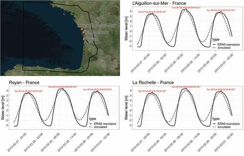
Figure A2. Storm Xaver (2013). Water levels from ERA5-reanalysis and ANUGA simulations.

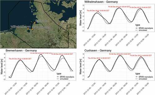
Figure A3. Storm surge in Emilia-Romagna (2002). Water levels from historical observations and ANUGA simulations.

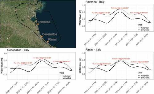
Appendix B

Table

System	Sub-system	Key	Value	Reclassification	Datatype
Energy		power	cable	cable	polyline
		power	minor_cable*	cable	polyline
		power	line	line	polyline
		power	minor_line	minor line	polyline
		power	plant	plant	polygon
		power	substation	substation	polygon
		power	tower	power tower	point
		power	pole	power pole	point
Water	Water supply	man_made	water_tower	water tower	polygon
		man_made	water_well	water well	polygon
		man_made	reservoir_covered	reservoir covered	polygon
		man_made	water_works	water works	polygon
Waste	Solid waste	amenity	waste_transfer_station	waste collection station	polygon
	Water waste	man_made	wastewater_plant	water treatment plant	polygon
Transportation	Railway	railway	rail	railway	polyline
		railway	subway	railway	polyline
		railway	tram	railway	polyline
		railway	construction	railway	polyline
		railway	funicular	railway	polyline
		railway	light_rail	railway	polyline
		railway	narrow_gauge	railway	polyline
	Public roads	highway	motorway	motorway	polyline
		highway	motorway_link	motorway	polyline
		highway	motorway_junction	motorway	polyline
		highway	trunk	trunk	polyline
		highway	trunk_link	trunk	polyline
		highway	primary	primary	polyline
		highway	primary_link	primary	polyline
		highway	secondary	secondary	polyline
		highway	secondary_link	secondary	polyline
		highway	tertiary	tertiary	polyline
		highway	tertiary_link	tertiary	polyline
		highway	residential	other	polyline
		highway	road	other	polyline
		highway	unclassified	other	polyline
		highway	living_street	other	polyline
		highway	service	other	polyline
		highway	pedestrian	other	polyline
		highway	bus_guideway	other	polyline
		highway	escape	other	polyline
		highway	raceway	other	polyline
		highway	cycleway	other	polyline
		highway	construction	other	polyline
		highway	bus_stop	other	polyline
		highway	crossing	other	polyline
		highway	mini_roundabout	other	polyline
		highway	passing_place	other	polyline
		highway	rest_area	other	polyline
		highway	turning_circle	other	polyline
		highway	traffic_island	other	polyline
		highway	yes	other	polyline
		highway	emergency_bay	other	polyline
	Airports	aeroway	aerodome	airports	polygon
		aeroway	runway	airports	polyline
Telecommunication	Telecom	man_made	communications_tower	communication tower	point
		man_made	mast	mast	point
		man_made,tower:type	communication	communication tower	point
Health**	Healthcare	amenity	clinic	clinic	point
		amenity	clinic	clinic	polygon
		amenity	doctors	doctors	point
		amenity	doctors	doctors	polygon
		amenity	hospital	hospital	point
		amenity	hospital	hospital	polygon
		amenity	dentist	dentist	point
		amenity	dentist	dentist	polygon
		amenity	pharmacy	pharmacy	point
		amenity	pharmacy	pharmacy	polygon
		healthcare	doctor	doctors	point
		healthcare	doctor	doctors	polygon
		healthcare	pharmacy	pharmacy	point
		healthcare	pharmacy	pharmacy	polygon
		healthcare	hospital	hospital	point
		healthcare	hospital	hospital	polygon
		healthcare	clinic	clinic	point
		healthcare	clinic	clinic	polygon
		healthcare	dentist	dentist	point
		healthcare	dentist	dentist	polygon
		healthcare	physiotherapist	physiotherapist	point
		healthcare	physiotherapist	physiotherapist	polygon
		healthcare	alternative	alternative	point
		healthcare	alternative	alternative	polygon
		healthcare	laboratory	laboratory	point
		healthcare	laboratory	laboratory	polygon
		healthcare	optometrist	optometrist	point
		healthcare	optometrist	optometrist	polygon
		healthcare	rehabilitation	rehabilitation	point
		healthcare	rehabilitation	rehabilitation	polygon
		healthcare	blood_donation	blood donation	point
		healthcare	blood_donation	blood donation	polygon
		healthcare	birthing_center	birthing center	point
		healthcare	birthing_center	birthing center	polygon
Education	Education	amenity	college	college	polygon
		amenity	kindergarten	kindergarten	polygon
		amenity	library	library	polygon
		amenity	school	school	polygon
		amenity	university	university	polygon

For a complete overview of active tags: https://wiki.openstreetmap.org/wiki/Map_features

*The value minor_cable is not amongst the active tags presented by OSM. However, we found unique cable assets that were tagged as ‘minor’. Therefore, we decided to still include these tagged assets as ‘cable’. **The list of OSM tags is based on the list that the healthsites.io project defined on their OSM-WIKI page as of March 2020

Appendix C

Energy

Hazard United States (HAZUS) is a geographic information system-based tool for analyzing natural hazard risk, which is developed and freely distributed by the Federal Emergency Management Agency (FEMA). Specifically for flood risk, FEMA developed a technical manual that contains vulnerability information for various types of infrastructure. We apply the vulnerability curves and maximum damages for plants and substations developed by FEMA (2013).

We distinguish between lines and minor lines, whereby OSM categorizes lines as high-voltage overhead powerlines that are usually supported by towers or pylons, while minor lines are supported by poles used for low-voltage transmission. We use a vulnerability curve for overhead transmission and distribution (T&D) systems, which assumes that only little damage occurs due to flooding (FEMA, 2013; Miyamoto, 2019). Maximum damages were not provided by either FEMA (2013) and Miyamoto (2019). We therefore base our maximum damages on construction costs for overhead lines in urban (for lines) and rural (for minor lines) areas provided by Hall (2009). Flooding impacts the above grade equipment that the cables are connected with, and this failure may propagate into the whole energy circuit. For the power towers and power poles we apply the vulnerability curve for T&D systems. Again, maximum damages were not provided, and we therefore use constructions costs for power towers and poles. Midcontinent Interdependent System Operator (MISO) provides yearly reports with estimated costs for various energy assets, including power towers and poles. OSM describes power towers as assets that carry high-voltage overhead power lines, and are often constructed from steel, while power poles are often made from wood. For this reason, we use the construction costs for single- and double circuit steel towers built for a range of high-voltage overhead lines for determining the maximum damage for power towers, while we only use construction costs for wooden poles (single and double circuit) for determining the maximum damage for power poles.

Transportation

Huizinga et al. (2017) provides grid-based vulnerability curves for application to the road network that can be used in combination with maximum damages in euro/m2. A recently published article, which assesses the flood risk of the European network, made an object-based translation of these vulnerability data (Van Ginkel et al., 2021). As part of this assessment, Van Ginkel et al. (2021) calculated the maximum damage in millions of euros per kilometre for the infrastructure types: motorway, trunk, primary, secondary, tertiary, and other. The maximum damages are derived by multiplying the maximum damage per m2 provided by Huizinga et al. (2017) with estimated typical roads width per road type. We use the vulnerability curve provided by Huizinga et al. (2017) for the road network in combination with the maximum damages in length units for different road types proposed by Van Ginkel et al. (2021).

The vulnerability function for railway systems is based on Kellermann et al. (2015). Instead of a curve, they propose a staircase threshold-wise damage states to present the vulnerability of railways, whereby three stages of damage are classified. The railways are assumed to be a standard double-tracked railway cross-section that consists of the following elements: substructure, superstructure, catenary and signals. The first damage class relates to the substructure of the railway that is (partly) impounded by water, but results in only little damage. The second damage class assumes that the substructure and superstructure of a track segment is completely flooded, which is expected to result in damage to at least the substructure. The final class assumes damage to the superstructure, catenary and/or signals, and that complete restoration is needed for the standard cross-section of the affected track segment. The maximum damage for railways is based on construction costs for railways (diesel and electrified) that are proposed by Carruthers (2013).

Lastly, a vulnerability curve for airports is provided by Kok et al. (2005). They also provide a maximum damage value given in damage per exposed footprint of an airport (euro/m2). The usage of this in combination with the spatial airport data, that are extracted from OSM in polygon format, may lead to an overestimation of the direct damages to airports. These polygons represent the airports in its whole, including areas that are covered by structural components, but also areas that are less important for risk analysis (e.g., grass). We therefore decide to breakdown the direct damages to airports by presenting structural damages to terminals and runways. For terminals, we use the vulnerability curve of Kok et al. (2005) in combination with maximum damage based on construction costs estimated by Carruthers (2013). Due to absence of more specific vulnerability curves for runways, we apply the vulnerability curve of Huizinga et al. (2017) estimated for roads.

Telecommunication

The infrastructure types of communication tower and mast are represented by the system as ‘telecommunication’. More specific vulnerability data for telecom assets are still lacking in the current body of literature. Therefore, we apply the vulnerability curve for the power systems to telecom infrastructure, which has also been done in Kok et al. (2005). Communication towers are structures with greater heights (could be above 100m) and are used for transmitting a range of radio applications (e.g., television, radio, mobile phone). Communication towers are often made from concrete. In contrast, masts are usually smaller, narrow masts of only a few meters high, and are typically used for a single radio application. We use the vulnerability curve of FEMA (2013) that we also apply for large power towers for communication towers. We assume that only little damage occurs to large communication towers, and this is what this vulnerability curve embodies. We used this in combination with maximum damages for ‘other community facility’ provided by FEMA (2013) as no specific construction cost data were available for communication towers. On the other hand, we assume that masts are more vulnerable to flooding as they are smaller structures compared to communication towers. We therefore apply the vulnerability curve proposed by Kok et al. (2005) for electricity and communication systems, which assumes higher damage factors. The maximum damage of masts is based on construction costs provided by Simmons (2022) and Liebman (2018).

Waste

The waste system is subdivided into two subsystems: solid waste and water waste. The solid waste subsystem is represented by infrastructure types of waste transfer station and landfill, whereas the water waste subsystem is represented by water waste treatment plants. In the current body of literature, specific vulnerability data on the solid waste infrastructure types is still lacking. We therefore apply the vulnerability curve and maximum damage proposed by Huizinga et al. (2017) for industrial areas. Waste transfer stations are extracted from OSM as polygon data, and the maximum damage is given in damage per exposed footprint. Landfills are excluded from the direct risk assessment due to the difficulty of assessing their damage. On the other hand, we use vulnerability curves and maximum damage estimates specifically developed for water waste treatment plants provided by FEMA (2013). This vulnerability data assumes that minor clean-up and repair activities are required when flood level exceeds ground level, and major activities when inundation levels reach approximately 1 meter.

Water

The water system is represented by four infrastructure types, namely water tower, water well, reservoir covered, and water works. We apply vulnerability data provided by FEMA (2013) on the four infrastructure types. FEMA (2013) includes vulnerability curves and maximum damages for (potable) water systems. The infrastructure type reservoir covered are large man-made tanks for holding water. FEMA (2013) provides vulnerability data for storage tanks at ground level, elevated structures, and tanks that are below ground level. However, OSM does not specify the height of the assets. We therefore take the average of the vulnerability curves and maximum damages for the different storage tanks specified by FEMA (2013) and apply this to the infrastructure type reservoir covered. A water tower is a structure that contains a water tank at an altitude to pressurize the water distribution network. We apply the vulnerability curve and maximum damage for elevated water storage tanks, which assumes that these structures will not be damaged during a flood. Furthermore, we use the vulnerability data specifically defined for water wells, which assumes that electrical equipment and well openings are 1 meter above ground level, and that a well is not permanently contaminated after flooding. Water works are structures where drinking water is found and applied to the waterpipes network. The public supply of water is stored and treated in this system of buildings and pipes. The (potable) water systems section of FEMA (2013) does not specify any data on water works. We therefore use the average of the vulnerability curves and maximum damages provided for water treatment plants (open and closed structures) and apply this for water works.

Education

The education facilities are extracted from OSM as polygons. Huizinga et al. (2017) developed vulnerability data for commercial buildings, which include schools as well. We use the vulnerability curve and maximum damage specified as damage per exposed footprint (euro per m2) proposed by Huizinga et al. (2017).

Health

Health facilities are tagged in OSM as point and polygon features. We extracted both datatypes and transformed the point features into polygon features based on average health facilities footprints of the polygon features. We corrected for duplicates in the dataset by verifying whether overlaps exist between a point and polygon feature. The Huizinga et al. (2017) vulnerability data used for education facilities are applied on health facilities as well (as the category ‘commercial facilities’ also include hospitals).

Appendix D

Table

	Xynthia		Xaver		Emilia Romagna
	Million Euro	Relative	Million Euro	Relative	Million Euro	Relative
Education	0.17	1.7%	0.16	9%	1.35	11%
Energy	0.00	0.0%	0.03	2%	0.17	1%
Healthcare	0.06	0.6%	0.03	2%	0.69	6%
Telecommunication	0.00	0.0%	0.00	0%	0.00	0%
Transportation	9.06	89.8%	1.15	66%	2.11	17%
Waste	0.80	7.9%	0.37	21%	8.14	65%
Water	0.00	0.0%	0.00	0%	0.00	0%

References

- Aerts, J. C. J. H. (2018). A Review of Cost Estimates for Flood Adaptation. Water, 10(11), 1646. https://doi.org/10.3390/w10111646
- Azevedo de Almeida, B., & Mostafavi, A. (2016). Resilience of Infrastructure Systems to Sea-Level Rise in Coastal Areas: Impacts. Adaptation Measures, and Implementation Challenges. Sustainability, 8, 1115. https://doi.org/10.3390/su8111115
- Bamber, J. L., Oppenheimer, M., Kopp, R. E., Aspinall, W. P., & Cooke, R. M., 2019. Ice sheet contributions to future sea-level rise from structured expert judgment. Proceedings of the National Academy of Sciences 116, 11195–11200. https://doi.org/10.1073/pnas.1817205116
- Bars, D. L., Drijfhout, S., & Vries, H. D. (2017). A high-end sea level rise probabilistic projection including rapid Antarctic ice sheet mass loss. Environmental Research Letters, 12(4), 044013. https://doi.org/10.1088/1748-9326/aa6512
- Bassis, J. N., Berg, B., Crawford, A. J., & Benn, D. I. (2021). Transition to marine ice cliff instability controlled by ice thickness gradients and velocity. Science, 372(6548), 1342–1344. https://doi.org/10.1126/science.abf6271
- Bertin, X., Bruneau, N., Breilh, J. F., Fortunato, A. B., & Karpytchev, M. (2012). Importance of wave age and resonance in storm surges: The case Xynthia, Bay of Biscay. Ocean Modelling, 42, 16–30.
- Bricheno, L. M., & Wolf, J. (2018). Future wave conditions of Europe, in response to High-End Climate Change Scenarios. Journal of Geophysical Research: Oceans, 123(12), 8762–8791. https://doi.org/10.1029/2018JC013866
- Calafat, F. M., Wahl, T., Tadesse, M. G., & Sparrow, S. N. (2022). Trends in Europe storm surge extremes match the rate of sea-level rise. Nature, 603(7903), 841–845. https://doi.org/10.1038/s41586-022-04426-5
- Carruthers, R. C., 2013. What Prospects for transport infrastructure and impacts on growth in Southern and Eastern Mediterranean Countries?. MEDPRO Report No. 3 https://www.medpro-foresight.eu/ar/system/files/MEDPRO%20Rep%20No%203%20WP5%20Carruthers_1.pdf
- Charnock, H. (1955). Wind stress on a water surface. Quarterly Journal of the Royal Meteorological Society, 81(350), 639–640. https://doi.org/10.1002/qj.49708135027
- Chauveau, E., Chadenas, C., Comentale, B., Pottier, P., Blanlœil, A., Feuillet, T., Mercier, D., Pourinet, L., Rollo, N., Tillier, I., & Trouillet, B. (2017). Xynthia: Lessons learned from a catastrophe. Cybergeo: European Journal of Geography. https://doi.org/10.4000/cybergeo.28032
- Chester, M. V., Underwood, B. S., & Samaras, C. (2020). Keeping infrastructure reliable under climate uncertainty. Nature Climate Change, 10(6), 488–490. https://doi.org/10.1038/s41558-020-0741-0
- CPSL (2005). Coastal Protection and Sea Level Rise - Solutions for sustainable coastal protection in the Wadden Sea region. Wadden Sea Ecosystem No. 21. Common Wadden Sea Secretariat, Trilateral Working Group on Coastal Protection and Sea Level Rise (CPSL). Available at: https://www.waddensea-worldheritage.org/sites/default/files/2005_Ecosystem21_cpsl.pdf
- Dangendorf, S., Arns, A., Pinto, J. G., Ludwig, P., & Jensen, J. (2016). The exceptional influence of storm `Xaver’ on design water levels in the German Bight. Environmental Research Letters, 11(5), 054001. https://doi.org/10.1088/1748-9326/11/5/054001
- Dawson, R. J., Thompson, D., Johns, D., Wood, R., Darch, G., Chapman, L., Hughes, P. N., Watson, G. V. R., Paulson, K., Bell, S., Gosling, S. N., Powrie, W., & Hall, J. W. (2018). A systems framework for national assessment of climate risks to infrastructure. Philosophical Transactions. Series A, Mathematical, Physical, and Engineering Sciences, 376. https://doi.org/10.1098/rsta.2017.0298
- DeConto, R. M., & Pollard, D. (2016). Contribution of Antarctica to past and future sea-level rise. Nature, 531(7596), 591–597. https://doi.org/10.1038/nature17145
- DEFRA. (2015). Adapting to Coastal Erosion Evaluation of rollback and leaseback schemes in Coastal Change Pathfinder projects. Department for Environment, Food and Rural Affairs.
- Deutschländer, D. T., Friedrich, K., Haeseler, D. S., & Lefebvre, C., 2013. Severe storm XAVER across Northern Europe from 5 to 7 December 2013 19. Deutscher Wetterdienst. https://www.dwd.de/EN/ourservices/specialevents/storms/20131230_XAVER_europe_en.pdf?__blob=publicationFile&v=4
- Evans, E. P., Ashely, R., Hall, J. W., Penning-Rowsell, E., Saul, A., Sayers, P. B., Thorne, C. R., & Watkinson, A. (2004). Future flooding - scientific summary. Volume 2 - Managing future risks. Office of Science and Technology.
- FEMA. (2013). Multi-hazard loss estimation methodology: Flood model HAZUS-MH MR3 technical manual. Department of Homeland Security, Federal Emergency Management Agency, Mitigation Division, Washington, D.C.
- Fenn, T., Garrett, L., Daly, E., Elding, C., Fleet, D., Udo, J., & Hartman, M., 2014. Study on economic and social benefits of environmental protection and resource efficiency related to the European semester: Final report. Publications Office of the European Union, LU.
- Forzieri, G., Bianchi, A., Silva, F. B. E., Marin Herrera, M. A., Leblois, A., Lavalle, C., Aerts, J. C. J. H., & Feyen, L. (2018). Escalating impacts of climate extremes on critical infrastructures in Europe. Global Environmental Change, 48, 97–107. https://doi.org/10.1016/j.gloenvcha.2017.11.007
- Garschagen, M., & Sandholz, S. (2018). The role of minimum supply and social vulnerability assessment for governing critical infrastructure failure: Current gaps and future agenda. Natural Hazards and Earth System Sciences, 18(4), 1233–1246. https://doi.org/10.5194/nhess-18-1233-2018
- Geoportale Nazionale., 2015. Project PST- Lidar Data. Geoportale Nazionale. http://www.pcn.minambiente.it/mattm/en/pst-project-lidar-data/ ( accessed 8.19.22)
- Haasnoot, M., Kwadijk, J., Alphen, J. V., Bars, D. L., Hurk, B. V. D., Diermanse, F., Spek, A. V. D., Essink, G. O., Delsman, J., & Mens, M. (2020). Adaptation to uncertain sea-level rise$\mathsemicolon$ how uncertainty in Antarctic mass-loss impacts the coastal adaptation strategy of the Netherlands. Environmental Research Letters, 15(3), 034007. https://doi.org/10.1088/1748-9326/ab666c
- Haklay, M., & Weber, P. (2008). OpenStreetMap: User-generated street maps. IEEE Pervasive Computing, 7(4), 12–18. https://doi.org/10.1109/MPRV.2008.80
- Han, Y., & Mozumder, P. (2021). Building-level adaptation analysis under uncertain sea-level rise. Climate Risk Management, 32, 100305. https://doi.org/10.1016/j.crm.2021.100305
- Hazeleger, W., van den Hurk, B. J. J. M., Min, E., van Oldenborgh, G. J., Petersen, A. C., Stainforth, D. A., Vasileiadou, E., & Smith, L. A. (2015). Tales of future weather. Nature Climate Change, 5(2), 107–113. https://doi.org/10.1038/nclimate2450
- Huizinga, J., Moel, H. D., & Szewczyk, W. (2017). Global flood depth-damage functions: Methodology and the database with guidelines (No. JRC105688), JRC Research Reports, JRC research reports. Joint Research Centre (Seville Site). doi:10.2760/16510.
- Kalra, N., Hallegatte, S., Lempert, R., Brown, C., Fozzard, A., Gill, S., & Shah, A. (2014). Agreeing on robust decisions : New processes for decision making under deep uncertainty. World Bank. https://doi.org/10.1596/1813-9450-6906
- Kellermann, P., Schöbel, A., Kundela, G., & Thieken, A. H. (2015). Estimating flood damage to railway infrastructure – The case study of the march river flood in 2006 at the Austrian Northern Railway. Natural Hazards and Earth System Sciences, 15(11), 2485–2496. https://doi.org/10.5194/nhess-15-2485-2015
- Kernkamp, H. W. J., Van Dam, A., Stelling, G. S., & de Goede, E. D. (2011). Efficient scheme for the shallow water equations on unstructured grids with application to the Continental Shelf. Ocean Dynamics, 61(8), 1175–1188. https://doi.org/10.1007/s10236-011-0423-6
- Kettle, A. J. (2020). Storm Xaver over Europe in December 2013: Overview of energy impacts and North Sea events. Advances in Geosciences, 54, 137–147.
- Kok, M., Huizinga, J., Vrouwenvelder, A. C. W. M., & Barendregt, A., 2005. Standard method 2004 damage and casualties caused by flooding [WWW Document]. (accessed September.20.22). Highway and Hydraulic Engineering Department, Delft. https://puc.overheid.nl/rijkswaterstaat/doc/PUC_116018_31/
- Koks, E. E., Nirandjan, S., Le Bars, D., Hrast-Essenfelder, A., & Sayers, P. (2021). The assessment of flood risk under the current climate for three storylines (No. D7.2). RECEIPT Deliverable. European Commission.
- Koks, E. E., Pant, R., Thacker, S., & Hall, J. W. (2019a). Understanding business disruption and Economic losses due to electricity failures and flooding. International Journal of Disaster Risk Science, 1–18. doi:10.1007/s13753-019-00236-y.
- Koks, E. E., Rozenberg, J., Zorn, C., Tariverdi, M., Vousdoukas, M., Fraser, S., Hall, J., & Hallegatte, S. (2019b). A global multi-hazard risk analysis of road and railway infrastructure assets. Nature Communications, 10(1), 1–11. https://doi.org/10.1038/s41467-019-10442-3
- Kolen, B., Slomp, R., & Jonkman, S. N. (2013). The impacts of storm Xynthia February 27–28, 2010 in France: Lessons for flood risk management. Journal of Flood Risk Management, 6(3), 261–278. https://doi.org/10.1111/jfr3.12011
- Kolen, B., Slomp, R., Van Balen, W., Terpstra, T., Bottema, M., & Nieuwenhuis, S., 2010. Learning from French experiences with storm Xynthia; damages after a flood. HKV LIJN IN WATER and Rijkswaterstaat, Waterdienst.
- Kulp, S. A., & Strauss, B. H. (2018). CoastalDEM: A global coastal digital elevation model improved from SRTM using a neural network. Remote Sensing of Environment, 206, 231–239. https://doi.org/10.1016/j.rse.2017.12.026
- Le Bars, D. (2018). Uncertainty in sea level rise projections due to the dependence between contributors. Earth’s Future, 6(9), 1275–1291. https://doi.org/10.1029/2018EF000849
- Levermann, A., Winkelmann, R., Albrecht, T., Goelzer, H., Golledge, N. R., Greve, R., Huybrechts, P., Jordan, J., Leguy, G., Martin, D., Morlighem, M., Pattyn, F., Pollard, D., Quiquet, A., Rodehacke, C., Seroussi, H., Sutter, J., Zhang, T., Van Breedam, J., … van de Wal, R. S. W. (2020). Projecting Antarctica’s contribution to future sea level rise from basal ice shelf melt using linear response functions of 16 ice sheet models (LARMIP-2). Earth System Dynamics, 11(1), 35–76. https://doi.org/10.5194/esd-11-35-2020
- Liebman, D. J., 2018. Cell tower leases add big value with little maintenance [WWW Document]. (accessed September.20.22). https://blog.sior.com/cell-tower-leases-add-big-value-with-little-maintenance
- Lin, B. B., Capon, T., Langston, A., Taylor, B., Wise, R., Williams, R., & Lazarow, N. (2017). Adaptation pathways in coastal case studies: Lessons learned and future directions. Coastal Management, 45(5), 384–405. https://doi.org/10.1080/08920753.2017.1349564
- Little, C. M., Urban, N. M., & Oppenheimer, M., 2013. Probabilistic framework for assessing the ice sheet contribution to sea level change. Proceedings of the National Academy of Sciences 110, 3264–3269. https://doi.org/10.1073/pnas.1214457110
- Lorie, M., Neumann, J. E., Sarofim, M. C., Jones, R., Horton, R. M., Kopp, R. E., Fant, C., Wobus, C., Martinich, J., O’Grady, M., & Gentile, L. E. (2020). Modeling coastal flood risk and adaptation response under future climate conditions. Climate Risk Management, 29, 100233. https://doi.org/10.1016/j.crm.2020.100233
- Marshall, T., & Cowell, R. (2016). Infrastructure, planning and the command of time. Environment and Planning C: Government and Policy, 34(8), 1843–1866. https://doi.org/10.1177/0263774X16642768
- May, P., Emonson, P., Jones, B., & Davies, A. (2014). Post-Installation effectiveness of property level flood protection (No. Final report FD2668). Department for Environment Food & Rural Affairs.
- Merkens, J.-L., Reimann, L., Hinkel, J., & Vafeidis, A. T. (2016). Gridded population projections for the coastal zone under the shared socioeconomic pathways. Global and Planetary Change, 145, 57–66. https://doi.org/10.1016/j.gloplacha.2016.08.009
- Miyamoto., 2019. Overview of Engineering Options for Increasing Infrastructure Resilience : Final Report [WWW Document]. World Bank. (accessed September.20.22). https://documents.worldbank.org/en/publication/documents-reports/documentdetail/474111560527161937/Final-Report
- Muis, S., Verlaan, M., Winsemius, H. C., Aerts, J. C. J. H., & Ward, P. J. (2016). A global reanalysis of storm surges and extreme sea levels. Nature Communications, 7(1), 11969. https://doi.org/10.1038/ncomms11969
- Nazarnia, H., Nazarnia, M., Sarmasti, H., & Wills, W. O. (2020). A systematic review of civil and environmental infrastructures for coastal adaptation to sea level rise. Civil Engineering Journal, 6(7), 1375–1399. https://doi.org/10.28991/cej-2020-03091555
- Nirandjan, S., Koks, E. E., Ward, P. J., & Aerts, J. C. J. H. (2022). A spatially-explicit harmonized global dataset of critical infrastructure. Scientific Data, 9(1), 150. https://doi.org/10.1038/s41597-022-01218-4
- O’Neill, B. C., Kriegler, E., Riahi, K., Ebi, K. L., Hallegatte, S., Carter, T. R., Mathur, R., & van Vuuren, D. P. (2014). A new scenario framework for climate change research: The concept of shared socioeconomic pathways. Climatic Change, 122(3), 387–400. https://doi.org/10.1007/s10584-013-0905-2
- Perini, L., Calabrese, L., Deserti, M., Valentini, A., Ciavola, P., & Armaroli, C. (2011). Le mareggiate e gli impatti sulla costa in Emilia-Romagna 1946-2010. Arpa Emilia-Romagna. ISBN: 88-87854-27-5. Available at: https://ambiente.regione.emilia-romagna.it/it/geologia/geologia/costa/pdf/atlantemareggiatecompletoweb.pdf/@@download/file/atlantemareggiatecompletoweb.pdf
- Reguero, B. G., Beck, M. W., Bresch, D. N., Calil, J., Meliane, I., & Añel, J. A. (2018). Comparing the cost effectiveness of nature-based and coastal adaptation: A case study from the Gulf Coast of the United States. PLOS ONE, 13(4), e0192132. https://doi.org/10.1371/journal.pone.0192132
- RMS., 2014. 2013–2014 Winter Storms in Europe: An insurance and catastrophe modeling perspective.
- Roberts, S., Nielsen, O., Gray, D., Sexton, J., & Davies, G. (2015). ANUGA user manual. Commonwealth of Australia (Geoscience Australia) and the Australian National University, 127.
- Rucińska, D. (2019). Describing Storm Xaver in disaster terms. International Journal of Disaster Risk Reduction, 34, 147–153. https://doi.org/10.1016/j.ijdrr.2018.11.012
- Sayers, P., Gersonius, B., Özerol, G., Nugraha, E., & Schipper, C. A. (2022a). A framework for cloud to coast adaptation: Maturity and experiences from across the North Sea. Land, 11(6), 950. https://doi.org/10.3390/land11060950
- Sayers, P., Moss, C., Carr, S., & Payo, A. (2022b). Responding to climate change around England’s coast - The scale of the transformational challenge. Ocean & Coastal Management, 225, 106187. doi:10.1016/j.ocecoaman.2022.106187.
- Sayers, P., Yuanyuan, L., Galloway, G., Penning-Rowsell, E., Fuxin, S., Kang, W., Yiwei, C., & Le Quesne, T. (2013). Flood risk management: A strategic approach. UNESCO.
- Shepherd, T. G., Boyd, E., Calel, R. A., Chapman, S. C., Dessai, S., Dima-West, I. M., Fowler, H. J., James, R., Maraun, D., Martius, O., Senior, C. A., Sobel, A. H., Stainforth, D. A., Tett, S. F. B., Trenberth, K. E., van den Hurk, B. J. J. M., Watkins, N. W., Wilby, R. L., & Zenghelis, D. A. (2018). Storylines: An alternative approach to representing uncertainty in physical aspects of climate change. Climatic Change, 151(3–4), 555–571. https://doi.org/10.1007/s10584-018-2317-9
- Sillmann, J., Shepherd, T. G., van den Hurk, B., Hazeleger, W., Martius, O., Slingo, J., & Zscheischler, J. (2021). Event-based storylines to address climate risk. Earth’s Future, 9(2), e2020EF001783. https://doi.org/10.1029/2020EF001783
- Simmons, A., 2022. How much does it cost to build a cell tower? Dgtl Infra. (accessed September.20.22). https://dgtlinfra.com/how-much-does-it-cost-to-build-a-cell-tower/
- Slangen, A. B. A., Carson, M., Katsman, C. A., van de Wal, R. S. W., Köhl, A., Vermeersen, L. L. A., & Stammer, D. (2014). Projecting twenty-first century regional sea-level changes. Climatic Change, 124(1–2), 317–332. https://doi.org/10.1007/s10584-014-1080-9
- Sözüer, M., & Spang, K. (2014). The importance of project management in the planning process of transport infrastructure projects in Germany. Procedia - Social and Behavioral Sciences, 119, 601–610. https://doi.org/10.1016/j.sbspro.2014.03.067
- Spencer, T., Brooks, S. M., Evans, B. R., Tempest, J. A., & Möller, I. (2015). Southern North Sea storm surge event of 5 December 2013: Water levels, waves and coastal impacts. Earth-Science Reviews, 146, 120–145. https://doi.org/10.1016/j.earscirev.2015.04.002
- Sterl, A., Bakker, A. M. R., Brink, H. W. V. D., Haarsma, R., Stepek, A., Wijnant, I. L., & Winter, R. C. D. (2015). Large-scale winds in the southern North Sea region: The wind part of the KNMI’14 climate change scenarios. Environmental Research Letters, 10(3), 035004. https://doi.org/10.1088/1748-9326/10/3/035004
- Thierry, S., Dick, S., George, S., Benoit, L., & Cyrille, P. (2019). EMODnet Bathymetry a compilation of bathymetric data in the European waters. OCEANS 2019 - Marseille Presented at the OCEANS 2019:. pp. 1–7. Available at: https://ieeexplore.ieee.org/abstract/document/8867250. https://doi.org/10.1109/OCEANSE.2019.8867250
- Tiggeloven, T., de Moel, H., Winsemius, H. C., Eilander, D., Erkens, G., Gebremedhin, E., Diaz Loaiza, A., Kuzma, S., Luo, T., Iceland, C., Bouwman, A., van Huijstee, J., Ligtvoet, W., & Ward, P. J. (2020). Global-scale benefit–cost analysis of coastal flood adaptation to different flood risk drivers using structural measures. Natural Hazards and Earth System Sciences, 20(4), 1025–1044. https://doi.org/10.5194/nhess-20-1025-2020
- Van den Hurk, B., Bisaro, A., Haasnoot, M., Nicholls, R. J., Rehdanz, K., & Stuparu, D. (2022). Living with sea-level rise in North-West Europe: Science-policy challenges across scales. Climate Risk Management, 35, 100403. https://doi.org/10.1016/j.crm.2022.100403
- Van Ginkel, K. C. H., Dottori, F., Alfieri, L., Feyen, L., & Koks, E. E. (2021). Flood risk assessment of the European road network. Natural Hazards and Earth System Sciences, 21(3), 1011–1027. https://doi.org/10.5194/nhess-21-1011–2021
- Vousdoukas, M. I., Mentaschi, L., Hinkel, J., Ward, P. J., Mongelli, I., Ciscar, J.-C., & Feyen, L. (2020). Economic motivation for raising coastal flood defenses in Europe. Nature Communications, 11(1), 2119. https://doi.org/10.1038/s41467-020-15665-3
- Vousdoukas, M. I., Mentaschi, L., Voukouvalas, E., Bianchi, A., Dottori, F., & Feyen, L. (2018). Climatic and socioeconomic controls of future coastal flood risk in Europe. Nature Climate Change, 8(9), 776–780. https://doi.org/10.1038/s41558-018-0260-4
- Vries, H. D., Katsman, C., & Drijfhout, S. (2014). Constructing scenarios of regional sea level change using global temperature pathways. Environmental Research Letters, 9(11), 115007. https://doi.org/10.1088/1748-9326/9/11/115007
- Wadey, M. P., Haigh, I. D., Nicholls, R. J., Brown, J. M., Horsburgh, K., Carroll, B., … Bradshaw, E. (2015). A comparison of the 31 January–1 February 1953 and 5–6 December 2013 coastal flood events around the UK. Frontiers in Marine Science, 2, 84.
- Weatherall, P., Marks, K. M., Jakobsson, M., Schmitt, T., Tani, S., Arndt, J. E., Rovere, M., Chayes, D., Ferrini, V., & Wigley, R. (2015). A new digital bathymetric model of the world’s oceans. Earth and Space Science, 2(8), 331–345. https://doi.org/10.1002/2015EA000107
- Winsemius, H. C., Aerts, J. C. J. H., van Beek, L. P. H., Bierkens, M. F. P., Bouwman, A., Jongman, B., Kwadijk, J. C. J., Ligtvoet, W., Lucas, P. L., van Vuuren, D. P., & Ward, P. J. (2016). Global drivers of future river flood risk. Nature Climate Change, 6(4), 381–385. https://doi.org/10.1038/nclimate2893
- Yan, K., Muis, S., Irazoqui Apecechea, M., & Verlaan, M., 2020. Water level change time series for the European coast from 1977 to 2100 derived from climate projections. Copernicus Climate Data Store. https://doi.org/10.24381/CDS.8C59054F
- Zoppou, C., & Roberts, S. (1999). Catastrophic collapse of water supply reservoirs in Urban areas. Journal of Hydraulic Engineering, 125(7), 686–695. https://doi.org/10.1061/(ASCE)0733-9429(1999)125:7(686)