Decoupled net present value: protecting assets against climate change risk by consistently capturing the value of resilient and adaptable investments

1

ABSTRACT

There is growing awareness that traditional valuation methods based on discounted cash flows using constant risk-adjusted discount rates struggle to account for climate-related risks when assessing long-term investments in physical assets and infrastructure. Worst yet, such methods fail to consider numerous financial benefits accruing from investment in resilience and adaptation, categorizing such expenditures as sunk costs that reduce investors’ returns. Such traditional valuation methods encourage investors to postpone or forgo entirely investing in resilience and adaptation. The decoupled net present value (DNPV) method incorporates risk and risk-reduction measures into project valuations in clear and compelling financial terms. By quantifying both (i) risk exposures of assets to hazards and (ii) the reduction of such exposure through up-front investments, DNPV recasts the financial impact of risk-reduction measures. Thus, the benefits of risk-reducing investments such as adaptation and resilience can be fully valorized in project-level accounting, removing a significant barrier facing such investments today.

KEYWORDS:

• Valuation
• DNPV
• Long-term investments
• climate change risk

1. Introduction

Worldwide economic losses from extreme weather events have increased steadily since the 1980s and was reported to sit approximately at a staggering $250–$300 billion annually in 2019 and will likely increase to $415 billion by 2030 (Hill et al., 2019), making an ever more compelling case for investments that build in flexibility and resilience and help enhance ex ante disaster reduction management. Likewise, by 2100 the value of global assets within the future 1-in-100-year coastal floodplains is projected to be between $7.9 trillion and $12.7 trillion (2011 value) under Representative Concentration Pathway 4.5 (RCP4.5),¹ rising to between $8.8 trillion and $14.2 trillion under RCP8.5 (IPCC, 2022). There is broad consensus among the scientific and regulatory communities that the physical impacts of climate change will increase the risk of losses in coming decades (Field et al., 2012; IPCC, 2018; UNEP, 2021) and the investment needed for a low-carbon, climate-resilient infrastructure (existing and new) is estimated to be at about $6 trillion per year (Schub et al., 2016), which is equivalent to 15% of the total global equity traded in 2021.

According to some estimates, the impact of climate change on asset values under business-as-usual scenarios could result in write-downs on the order of 17% of global financial asset value (Dietz et al., 2016). As such, deployment of capital to develop resilient and adaptable assets in multiple sectors of the economy to reduce climate risk exposure will be critical to the sustainability of both the private and public sectors. This has been recognized for some time by governments of many countries, and policies are being developed to better quantify the vulnerability of key infrastructure to the impacts of climate change and develop strategies for improving resilience. Likewise, multilateral lenders have increased their focus on promoting climate-change-resilient infrastructure (Bouskela et al., 2016; JRMDB, 2020). Furthermore, to optimize resource allocations and reduce initial costs given the uncertainty of future climate impacts, flexible and adaptive approaches can reduce the costs of incorporating climate resilience into infrastructure investments, as documented in a recent report (Carmody & Chavarot, 2021). The report, prepared by the Coalition for Climate Resilient Investment (CCRI), also describes the increasing awareness within the investment community of the potential risks posed by climate change and the need for innovative sustainable investment practices, including the need for a new paradigm regarding asset valuation and long-term investment plans (page 41).

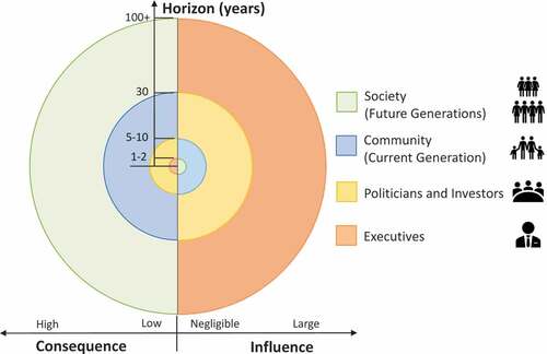
In a speech to Lloyds Bank of London, the then-Governor of the Bank of England Mark Carney warned that the catastrophic impact of climate change will be felt well beyond the typical horizon of investment and political cycles, imposing a cost on future generations that the current generation (community and decision makers alike) has little incentive to avoid (Bank of England, 2015). Carney coined the term ‘the tragedy of the horizon’ to describe this state of affairs. The use of Discounted Cash Flows (DCF) techniques with inflated and poorly conceived risk-adjusted discount rates to evaluate long-term investment opportunities further aggravates the tragedy because it artificially emphasizes short-term costs (which can be ‘reduced’ by postponing them) as well as short-term revenues (which are encouraged to be generated sooner) while significantly undervaluing future assets and liabilities and substantially downplaying future risks. As a result, stakeholders with shorter investment horizons yet outsized influence (e.g., corporate executives, investors, bankers, government officials, and politicians) frequently promote myopic strategies suitable to their short-term horizons and tend to select projects with initial high returns over those that would yield higher long-term stakeholder value (Antia et al., 2010; Lundstrum, 2002). And they do so without a clear understanding of the embedded, and often accumulating, investment risks. This is a problem both when infrastructure assets are initially planned and when it is sold or transferred among investors. Unfortunately, the imbalance between stakeholders’ time horizon and influence is the norm rather than the exception (Figure 1). Thus, to alleviate the tragedy of the horizon by promoting investments in resilient and adaptation, not only a change in the stakeholders’ mindset but also a paradigm shift in asset valuation methods will be required. Specifically, the fundamental, albeit unsupported, tenet of investment valuation (i.e., accounting for risks in the discount rates to render future uncertain cash flows riskless and in today’s value) need to be called into question.

Figure 1. Horizon impact/Stakeholder’s influence chart.

2. Making the case against conventional DCF techniques

Most investors are risk averse and prefer cash flows that are certain over those that are uncertain (i.e., riskier). Likewise, most people confer higher value to goods received sooner than those received later – the farther into the future, the lower their value. When the goods considered is money, the time-preference effect is known as the time value of money (TVM). Thus, both risk and TVM reduce (i.e., discount) the value of future uncertain cash flows. Many decision-makers rely on DCF approaches to establish the financial viability of capital investment projects. The basic DCF premise is that the value of future cash flows deemed risky or uncertain can be discounted to obtain equivalent cash flows expressed in risk-free terms and in today’s dollars such that they can be subsequently added and subtracted. The sum of all future cash flows (revenues and costs) discounted to account for risk and TVM to attain their present value is known as the net present value (NPV). This is typically accomplished by selecting a single risk-adjusted discount rate (α) to account for two fundamentally different phenomena when calculating the present value of future cash flows: TVM and the aggregate project-specific risks. As such, discount rates become a proxy for all risks affecting the investment, which are selected based on convention, heuristic arguments, and rules of thumb. For instance, corporations often prescribe the discount rates to be used when evaluating capital investment projects based on their weighted average cost of capital (WACC), which is calculated as the weighted cost of debt and equity, and it is further adjusted (i.e., increased) to account for actual or perceived project-specific risks. Often, WACC is equated to the TVM. In essence, traditional DCF mixes TVM and risk, indicating that they are interchangeable,² and any risk (regardless of its source) can be described by the same expression³ with a singular parameter (i.e., α). The two most popular DCF decision-making approaches for investing are (i) the NPV rule, that is, invest if NPV ≥ 0; and (ii) the internal rate of return (IRR) rule, that is, invest if IRR ≥ α.

The main features of the DCF approaches, which rely on a seemingly innocuous and expedient function used to calculate discounting factors, are that NPV decreases rapidly as time and discount rate increase. Since higher discount rates often chosen for riskier investments also have the consequence of reducing the value of future expenditures and losses (e.g., climate risks), it follows that simply increasing the discount rate to account for risk often achieves the opposite: expenditures and risks are discounted. Furthermore, the cavalier and unscientific approach typically used to assign a risk premium to the discount rate frequently results in unduly high discounting. As a consequence, the higher the selected discount rate, the larger the time bias effect overstating short-term values and underestimating long-term ones.

As a result, investing in resilience and adaptation to avoid future losses is harder to justify when using DCF-based approaches even when physical climate risks will increase in severity over time and so-called robust approached are used to evaluate multiple severe scenarios. Further drawbacks of the DCF accounting approach with implications for investment in climate resilience include (i) the inability to assess and assign value to varying levels of uncertainty and dispersion of possible future cash flow outcomes and (ii) the failure to distinguish in the discounting process between systematic risks and project-specific, idiosyncratic risks makes it impossible to assess the effectiveness of different risk management measures (e.g., reduction, transferring, avoiding, sharing).

Although the limitations of DCF and the dangers of adjusting discount rates for risk have been known for nearly 60 years (e.g., Robichek & Myers, 1966), because the DCF method is simple and readily applied to project and corporate accounting, it quickly took off; therefore, the practice of accounting for risk in discount rates prevailed in academia and practice. Even when the shortcomings of DCF are recognized and criticized, proposed solutions are still based on risk adjusted discount rates (e.g., Lilford et al., 2018). As a result, investment performance continues to be evaluated and decisions continues to be made using DCF techniques. Moving away from well-established (albeit flawed) practices takes significant time and effort, particularly when existing methods are simple and expedient, easy to communicate to decision-makers, and even deeply rooted in public policy.⁴ In addition, sectors of the economy that currently benefit from the status quo cannot be counted on to support the adoption of disruptive ideas.

Compounding the problem, DCF implicitly assumes that investment decisions are one-time irrevocable events made at the start of the investment (e.g., invest if NPV > 0, otherwise pass) assuming a fixed period and unchangeable multiyear cash flow layout with a constant expected annual return. In other words, DCF unrealistically assumes that once the initial investment decision is made, no changes can be made in response to deviations of the assumed conditions. Since resilient and adaptive infrastructure provides management with flexibility to make changes in the future as uncertainty gets resolved, it is clear that the principles upon which DCF techniques were developed makes them unsuitable to value resilient and adaptive assets.

In summary, DCF approaches to valuing infrastructure assets do not accurately model climate risk because they:

1. Devalue longer-term liabilities even when highly certain;

2. Overemphasize the value of near-term revenues and expenditures, thereby incentivizing short-term decision-making;

3. Disproportionately compensate those carrying ‘early’ risks;

4. Do not distinguish between systemic and idiosyncratic risks, even as management of the latter can reduce project risk, thereby encouraging investment in climate resilience and de-risking the project as a whole;

5. Assign expected values that are unreflective of often substantial uncertainties, risks, and variances in future cash flow projections, thereby failing to capture the ‘risk discount’ of uncertain future cash flows;

6. Assume investment decisions are a singular moment in time; and

7. Struggle to incorporate the value of flexibility.

As a result, to finance long-term projects using DCF analysis, investors may demand a higher return on investment disproportionate to the actual project risk while at the same time stifling the flow of capital needed to address longer-term physical climate risks, thus discouraging investments in resilience and adaption. This practice can lead to risk and wealth misallocation (i.e., unfair compensation) among existing and future stakeholders, essentially robbing future Peters to pay contemporary Pauls. Future generations are most vulnerable because they have no influence over today’s investment decisions yet stand to inherit the impacts thereof.

The economic impact under the status quo of unduly penalizing long-term projects and failing to internalize the benefits of risk-reduction actions to both investors and society is not trivial. Not addressing climate risk will disproportionally affect communities that can least afford it, adding to the existing inequality (Stiglitz & Stern, 2015). The deleterious and potentially catastrophic effects of climate change in sectors that are key to economic growth (e.g., energy, water, transportation, agriculture) have further accentuated the need to adopt long-term investment strategies. However, this will require moving away from using standard DCF methods along with prescribed risk-adjusted discount rates (Cifuentes & Espinoza, 2016; Espinoza, 2022). Fortunately, due in no small part to the significant threat imposed by climate change, visible efforts are directed toward addressing the issue of discounting (Carmody & Chavarot, 2021). Due to the shortcomings of the existing financial tools, a different risk quantification framework is clearly needed to address potential less-than-optimal capital allocations for longer-term climate adaptation and resilience measures (Thomä et al., 2015). Unfortunately, most of the proposed frameworks (e.g., robust decision-making, portfolio analysis) are still based on DCF approaches, that is, the main root of the problem (i.e., mixing risk with TVM) is left largely unanswered.

3. Discussion of new economic decision-making tools for adaptation investment evaluation

The limitations of traditional decision-making tools rooted in DCF techniques to evaluate resilience and adaptation investment strategies are widely recognized now in the literature and multiple approaches (e.g., robust decision-making, portfolio analysis, real options) are increasingly explored in the literature (Carmody & Chavarot, 2021; Dittrich et al., 2016; Guthrie, 2019; Kalra et al., 2014; Watkiss et al., 2015) to develop a solid framework to evaluate projects that account for the changing uncertainties associated with climate change. Unfortunately, except for real options, the proposed approaches are still based on the premise that risks can be accounted for in the discount rates. Further, these approaches assume that since climate change risk has not been incorporated in the discount rate, it can be treated differently from the other risks by developing cash flows probabilistic distributions for one or multiple climate scenarios. The difference among the different approaches is the manner these probabilistic distributions are manipulated to develop a decision-making framework.

For instance, robust decision-making methods involve testing strategies across a large number of possible futures using a wide range of climate scenarios. Cost benefit analysis for multiple scenarios are typically calculated using simulation models. Likewise, portfolio analysis attempts to reduce risk by adopting multiple adaptation options for a range of plausible future climate scenarios. Similar to stocks, risk is characterized as a variation of the return and the portfolio is optimized to obtain the highest return for a given risk or the lowest risk for a given return (measured in terms of NPV). Because portfolio analysis also requires evaluating multiple scenarios simulation models are typically used. Other similar approaches have been recently proposed. A summary of the advantages and disadvantages of these methods as applied to adaption can be found in the literature (e.g., Dittrich et al., 2016; Watkiss et al., 2015). The main drawback of these approaches is the inconsistent treatment of risks (most in the discount rate and climate change in the cash flows) that makes it difficult to interpret the results. Since typical risk adjusted discount rates are relatively high, as discussed above, the effect of climate change risk (considered in the cash flows) is rendered negligible.

From the methods discussed in the literature, real options analysis (ROA) is conceptually well suited for evaluating adaptation and resilience investments for multiple reasons: (1) Consistency. ROA accounts for all uncertainty including climate change through the use of probabilistic descriptions of cash flows; (2) Flexibility. ROA can capture the value of flexibility that may be attained by adopting different adaptation strategies depending upon how future climate unfolds; and (3) Separation of risk and TVM. ROA addresses the issue of discounting because all risks are calculated in monetary terms (i.e., the option value), thus therefore the TVM of cash flows can be discounted using risk-free rates. Although ROA appears to be the best decision-making tool to evaluate adaptation and resilient strategies, its application is not straight forward and may require considerable expertise to apply in practice (Dittrich et al., 2016).

4. Monte Carlo simulation is not the panacea to achieve robustness

As discussed above, the implementation of the new economic decision-making tools require Monte Carlo simulation, a computational technique that allows analysts to forecast the probability distribution of a function that depends on one or more random variables. Because this technique accounts for the variability associated with the cash flows, it is presumed that the uncertainty of the cash flows is also accounted for. The method consists of describing probabilistically key variables used to calculate the DCF and selecting the values of these variables randomly – hundreds or thousands of times – while keeping track of the outcomes (e.g., NPV, IRR) to calculate its probability distribution. As commercial software (e.g., @Risk, Crystal Ball) to perform Monte Carlo simulation becomes more ubiquitous and user-friendly, practitioners in many disciplines are becoming more accustomed to using this technique to evaluate risk.

However, Monte Carlo simulation applied to DCF-based decision-making analysis has multiple drawbacks that cannot be ignored before making financial decisions based on the results of simulation, namely the following:

1. Implementation difficulties: Because simulating cash flows can be very difficult, particularly for investments with embedded flexibility and path dependencies, they are often replaced with oversimplified unrealistic models.

2. Double-counting risk: Since NPV assumes the selection of an appropriate risk-adjusted discount rate (i.e., investment risks are already supposedly accounted for in the discount rate), the meaning of a NPV probability distribution is, at best, unclear and difficult to interpret and, at worst, pointless.

3. Inconsistency: Even for cases where the cash flow probabilistic distribution only accounts for risks not included in the discount rate (e.g., climate change), the inconsistent treatment of risk make the interpretation of the results difficult. In many cases, it makes the effect of climate change unrealistically negligible.

4. Valuation model error: Describing the cash flows probabilistically does not resolve the theoretical flaws of the NPV discussed above. Regardless of the number of simulations performed, the calculated NPV for each sampling event will incur the same time-bias effect and will typically fail to incorporate suitable risk-exposure discounting unless expressly added to the quantification of the simulation.

To illustrate this issue, we present a simplified example of a coastal 50-megawatt (MW) wind farm that consists of an initial investment of $130 M and is expected to yield an average cash flow of $14.5 M per year (in today’s dollars) for 20 years (Row A, Table 1). For simplicity, let’s assume that all the initial investment is deployed in year 0. Let’s further assume that the investor considered that α = 10% is the appropriate risk-adjusted discount rate (real) for this particular investment to calculate the DCF (Row B in Table 1).

Table 1. Cash flow analysis (in millions).

	Y0	Y1	Y2	Y3	…	Y18	Y19	Y20
A. Cash Flows	($130)	$14.50	$14.50	$14.50	…	$14.50	$14.50	$14.50
B. DCF	($130)	$13.18	$11.98	$10.89	…	$2.61	$2.37	$2.16

NPV = -$65.5 IRR = 9.3%

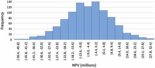
Thus, the deterministic NPV and IRR are calculated to be (-$6.55 M) and 9.3%, respectively. The deterministic analysis indicates that investment should not be made because NPV < 0 (i.e., IRR < α). Let’s assume that future cash flows can be described by a normal distribution with an annual expected revenue and a standard deviation of $14.5 M and $6.0 M, respectively, the results of a sample Monte Carlo simulation 1,000 times yield an expected NPV and IRR equal to (-$6.75 M) and 9.2%, respectively. The histogram distribution of the simulated NPVs for 1,000 iterations are represented in Figure 2.

Figure 2. Monte Carlo simulation for NPV.

As expected, since the valuation model (i.e., NPV) remained the same, the results were essentially the same as the deterministic calculation albeit with a lot more work. The added effort of the simulation did not provide additional useful information that could be used for decision-making. This is not an artifact of the relative simplicity of the example used. There would be a similar conclusion if more complex cash flow models were developed, including a complex decision tree analysis as it would be case with the so-called robust models. Many fail to notice this simple fact when evaluating Monte Carlo simulation results and make decisions thinking that risks have been duly accounted for. This does not imply that simulation is not useful, it merely points out to the fact that the main issues raised above about adding risk to the discount rate is not addressed by performing thousands (or millions) of simulation.

5. Pivoting to a robust risk quantification framework: decoupled net present value

Robichek and Myers (1966) indicated that adding the TVM and risk effects in a single parameter was not appropriate and proposed the certainty equivalent method. Building on this concept, Zeckhauser and Viscusi (2008) noted that the preferred approach to address risk should be to convert risky cash flows to certainty equivalent cash flows (i.e., expected cash flows reduced to account for risk) and then discount the reduced cash flows using risk-free rates (i.e., accounting for TVM of the already de-risked cash flows). An approach that does exactly that is the decoupled net present value (DNPV) method (Espinoza, 2014; Espinoza & Morris, 2013; Espinoza et al., 2020). The DNPV method introduces the concept of cost of risk,⁵ which is considered as an additional cost to the project, and it is used to calculate the certainty equivalent cash flows at each time period (t).

In simple terms, the cost of risk can be thought of as the fair price to compensate risk takers (e.g., investors) for the specific risks assumed. Considering risk as a cost to the project is a natural progression from the conventional business and personal practice of buying insurance products to protect against certain risks (e.g., home insurance, disability insurance, car insurance). The concept captures the downside potential of an investment and is included in the cash flows explicitly as a project cost. On any project, risks are classified within two main groups:

• Revenue Risk, which is defined as obtaining lower revenues than expected.

• Expenditure Risk, which is defined as incurring higher costs than originally expected.

There may be multiple contributory sources to each of these risks, which depend on the project under consideration. For example, in addition to typical commercial risks, merchant hydropower plants can be subjected to temporary or permanent shutdown related to contingency risks (e.g., spillway overflow that might damage the dam due to extreme rainfall events) that might affect revenues due to lower energy output or operating costs due to subsequent repairs. When dealing with climate change, risks are often classified as chronic (i.e., results in a longer-term permanent change of the probability distribution) or acute (i.e., lower-probability event driven). Regardless of the classification or nomenclature used to describe the risks, the cost of risk should be properly captured in the DNPV analysis.

Under DNPV, independent of its source, each risk has a cost. These costs are accounted for in the valuation process to reduce the value of the expected cash flow (i.e., the certainty equivalents). The advantage of using the cost of risk concept is that risks make certainty equivalent revenues smaller and certainty equivalent expenditures higher.⁶ Because the risks associated with the project are directly accounted for in the cash flows, the net certainty equivalent (i.e., riskless) cash flows, calculated as the certainty equivalent revenues minus certainty equivalent expenditures, can then be discounted using term-appropriate risk-free rates.⁷ This is summarized in Equation (1)(1) $\mathrm{D}\mathrm{N}\mathrm{P}\mathrm{V}=\sum _{t=0}^T\frac{{\tilde{V}}_t-{\tilde{E}}_t-R_t}{{\left(1+r\right)}^t}$(1) below.

(1) $\mathrm{D}\mathrm{N}\mathrm{P}\mathrm{V}=\sum _{t=0}^T\frac{{\tilde{V}}_t-{\tilde{E}}_t-R_t}{{\left(1+r\right)}^t}$(1)

where T is the asset life, ${\tilde{V}}_t$ and ${\tilde{E}}_t$ are the expected cash flows (revenues and expenditures, respectively) at time t, R_t represents the sum of the costs of risks at each time period, and r is the risk-free rate to account for TVM. By identifying individual components of risk, data can be compiled in a repository database in a manner conducive to analysis using data analytics techniques. This data can later serve to improve estimates of the cost of similar risks. The cost of risk assumed by investors represents their compensation for taking on such risks.

This approach separates risk from TVM and facilitates the evaluation of the effect of each source of risk (market and nonmarket) at different times during the life of the asset. In general, depending on the source of each risk and the availability of data to evaluate it, the cost of risk could be estimated using (i) probabilistic/stochastic methods based on probability density functions (PDFs) constructed from available empirical data; (ii) subjective industry-specific information obtained from technical experts; and/or (iii) option pricing techniques (Carmichael et al., 2011). In fact, DNPV has all the advantages identified in real options but the mechanics of its implementation is more straight forward and intuitive. The mechanics of cost of risk calculations and examples of applications can be found elsewhere (e.g., Espinoza & Morris, 2013; Espinoza & Rojo, 2015). To put it simply, the DNPV method is not only simple and intuitive but also flexible, consistent, and robust: it allows investors and project sponsors to explicitly model and quantify risk in financial terms (i.e., the cost of risk). The cost of risk has the appropriate features to gain prominence in the climate change decision-making process as DNPV combines features of real options and robust decision-making. Recognition that there might be more or different information in the future that can impact the infrastructure and considering upgradable resilient and adaptable features in the design provides significant flexibility to the developer. Like real options, the value added by this flexibility can be evaluated using DNPV. Similarly, because the computation of the cost of risk requires an assessment of the probability characteristics of the cash flows, each plausible future climate scenario identified can be associated with a corresponding cost of risk which can then be used to develop a resilience and adaptation strategy together with an implementation criteria.

6. The risk rate of return

One of the chief strengths of DNPV analysis is that by identifying and quantifying individual components of risk, there is no need to prescribe a discount rate (other than quoted risk-free rates). Nonetheless, to convey the results of the DNPV analysis in a simple manner using terms familiar to analysts and decision makers who are familiar with DCF approaches, the calculated project DNPV can be used together with Equation (2)(2) $\sum _{t=0}^T\frac{{\tilde{V}}_t-{\tilde{E}}_t}{{\left(1+RRR\right)}^t}=DNPV$(2) to back-calculate an equivalent risk-adjusted discount rate that is referred to as the risk rate of return (RRR):

(2) $\sum _{t=0}^T\frac{{\tilde{V}}_t-{\tilde{E}}_t}{{\left(1+RRR\right)}^t}=DNPV$(2)

The parameter RRR in Equation (2)(2) $\sum _{t=0}^T\frac{{\tilde{V}}_t-{\tilde{E}}_t}{{\left(1+RRR\right)}^t}=DNPV$(2) is constant for the period under consideration. Equation (2)(2) $\sum _{t=0}^T\frac{{\tilde{V}}_t-{\tilde{E}}_t}{{\left(1+RRR\right)}^t}=DNPV$(2) is equivalent to the NPV equation with RRR representing the average risk-adjusted discount rate that would make the NPV of the expected cash flows equal to the calculated DNPV. If all the risks associated with the cash flows have been identified and correctly quantified, DNPV calculated using Equation (1)(1) $\mathrm{D}\mathrm{N}\mathrm{P}\mathrm{V}=\sum _{t=0}^T\frac{{\tilde{V}}_t-{\tilde{E}}_t-R_t}{{\left(1+r\right)}^t}$(1) should represent the true value of the investment accounting for risk and TVM. In such a case, RRR can be viewed as the risk-adjusted discount rate that represents the asset’s average risk for the period of interest. Then, RRR can be compared with the investor’s target discount rate (α) typically used in DCF approaches.

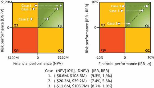
Rather than jettison the standard financial analysis and pivot to the proposed DNPV, the classic NPV is used as a measure of the project financial performance (i.e., the ability of the project’s cash flow to earn the investor’s WACC) whereas DNPV is used as a measure of the project risk performance. A project is said to earn a return consistent with the risk of the project if DNPV > 0 (or IRR > RRR). Likewise, the project is said to earn a return consistent with its cost of capital if NPV > 0 (or IRR ≥ α). This simple yet powerful concept can be illustrated in a cartesian plane (Figure 3) designated as Financial Performance-Risk Performance plots. As shown, the traditional DCF approaches (i.e., invest if NPV ≥ 0 or IRR ≥ α) is expanded to account for risk. In this framework, the parameter α no longer represents the risk-adjusted discount rate but more aptly represents the desired rate of return, that is, the return that investors would like to obtain if they were to invest in the project. Such desired return may or may not compensate them for the actual average investment risk (RRR), which is evaluated using DNPV. This two-pronged approach provides significantly greater insight to the successful outcome potential of investments in real assets.

Figure 3. Financial performance-Risk performance plots.

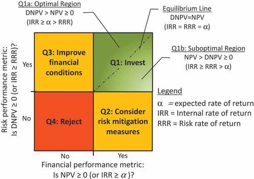
The results of multiple investment alternatives can be graphically represented in a NPV-DNPV axis (or alternatively in an incremental returns axis) and plotted on a chart similar to Figure 3. As shown in this figure, a given investment could plot in any of four quadrants:

1. Q1 corresponds to the investment region where both NPV > 0 (or IRR ≥ α) and DNPV > 0 (or IRR > RRR) with projects plotted above the equilibrium line being more desirable than those below.

2. Q2 represents the region where the investment financial performance target is met but needs improvement of the risk performance, meaning that investors should consider risk-management measures such as reduction, transferring, avoiding, sharing

3. Q3 represents the region where the investment meets the risk performance target but needs to improve its financial performance, indicating that investors should consider leverage with cheaper sources of capital, align return on equity demands with actual investment risks, or both.

4. Q4 represents the investment rejection region.

This plot can be used to illustrate whether or not investors are properly compensated for the risks taken. If the project cash flows are valued using α ≥ RRR, then investors will be overpaid for the project risks. On the other hand, if α < RRR, then investors are not properly compensated for the risks taken. The same project with different adaptable and resilient features can plot in different regions of Figure 3 reflecting the impact of such features in the probability distribution of the cash flows. This figure can be used to convey information to stakeholders regarding the advantages of investing in flexible and adaptable infrastructure. This is a significant departure from traditional valuation in the sense that the probability distributions of the cash flows are taken into consideration in a clear, consistent, and transparent manner.

7. Application example of proposed method

The simple wind farm example described above that resulted in NPV = (-$6.6 M) and IRR = 9.3% is analyzed here to illustrate the mechanics of DNPV for several cases.

7.1. Case 1: business as usual

The cash flows (Row A) are similar to those in a NPV analysis. For illustrative purposes, let’s assume that the cash flow variability in Figure 2 represents market risk and that the wind farm was designed to withstand typical weather events based on pre-climate-change climatological data. Thus, potential losses (i.e., reduction in cash flows) are only due to market conditions, not extreme weather events. Since annual cash flows are random variables described by a normal distribution, this information is used to estimate the cost of risk (Row B in the table below), that is, the project market risk expressed in monetary terms. The expected downside, $\tilde{D},$ is simply the average of all the values lower than the expected cash flows ($\tilde{V}$). The cost of risk is simply ($\tilde{V}-\tilde{D}$) times p, which is area below the expected cash flow (i.e., 0.5 since it is symmetrical). A graph depicting how the cost of risk is calculated is presented as Figure 4.

Figure 4. Cash flow probability distribution profile.

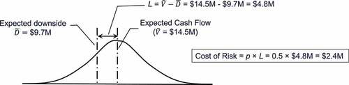
The riskless cash flows (Row C) are then calculated by subtracting the cost of risk (due to market uncertainty) from the cash flows (i.e., Row A – Row B). Since market risk was removed from the cash flows, the resulting cash flows in Row C is considered riskless and can be discounted using the risk-free rate. Since all cash flows are in today’s dollars, Treasury inflation-protected securities (TIPS) can be used to account for the TVM in real terms. For this particular example, a 10-year risk-free real rate (i.e., net of inflation) was used. The 10-year TIPS, quoted at 0.11%, is used to discount the riskless cash flows in Row C to calculate a DNPV of $108.6 M. Because market risk (i.e., $2.42 M per year) was accounted for in the cash flows, there was no need to adjust the risk-free rate to account for risk, thus avoiding double counting risk. Thus, DNPV resolves one of the issues associated with using the probability distribution of the cash flows.

Furthermore, the expected cash flows in Row A along Equation (2)(2) $\sum _{t=0}^T\frac{{\tilde{V}}_t-{\tilde{E}}_t}{{\left(1+RRR\right)}^t}=DNPV$(2) can be used to back-calculate RRR, the discount rate that would make the present values of the expected cash flows equal to DNPV (i.e., $108.6 M), that is, RRR = 1.9%. If the actual variability of the cash flows in Table 2 considering market risk only is described by a normal distribution, then the investor’s use of 10% as a discount rate to calculate the NPV would not be appropriate for the actual project risk. In this case, investors would be overcompensated for the risk taken (assuming market risk only).

Table 2. Business as usual case – no climate change (in millions).

	Y0	Y1	Y2	Y3	…	Y18	Y19	Y20
A. Cash Flows	($130)	$14.50	$14.50	$14.50	…	$14.50	$14.50	$14.50
B. Cost of risk (base case)		$2.42	$2.42	$2.42	…	$2.42	$2.42	$2.42
C. Riskless cash flow	($130)	$12.08	$12.08	$12.08	…	$12.08	$12.08	$12.08

7.2. Case 2: including climate change flood risk

Now, let’s assume that, based on revised climatological data, the wind farm critical infrastructure as currently designed is susceptible to flooding. To facilitate the discussion, it is assumed that flooding risk (which was previously assumed to be negligeable) is now subjected to a binary 10% chance of flooding in any given year (because of climate change) resulting in a temporary shutdown of 6 months with the associated reduction of cash flows of $7.25 M (0.5 × $14.5 M). In addition, flooding is expected to cause damages that result in $11.25 M of added expenditures (e.g., substation replacement). The total expected negative impact to cash flows due to flooding would be $18.5 M ($7.25 + $11.25). Hence, it follows that when flooding occurs, the expected cash flows should be -$4 M ($14.5 M – $18.5 M). Rather than assuming a specific year when flooding might occur and applying the reduced cash flow in that year, the probability description of the event is used to estimate the revised conditions. Therefore, if climate change is considered, the revised expected value of the cash flows for years 1–20 considering flooding is $12.65 M (see, Figure 5) – a reduction of $1.85 M. The NPV considering the lower expected cash flows (Row B in Table 3) is (-$20.3 M) with a corresponding IRR = 7.4%. Thus, according to the NPV > 0 rule, this is not an investment worth pursuing.

Figure 5. Estimate of revised expected value and cost of risk of flooding.

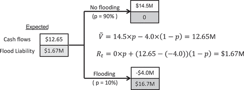
Table 3. Cash flows considering flooding (in millions).

	Y0	Y1	Y2	Y3	…	Y18	Y19	Y20
A. Expected cash flows (no flooding)	($130)	$14.50	$14.50	$14.50	…	$14.50	$14.50	$14.50
B. Expected cash flows (with flooding)	($130)	$12.65	$12.65	$12.65	…	$12.65	$12.65	$12.65
C. Cost of risk
(1) Base case (market)		$2.42	$2.42	$2.42	…	$2.42	$2.42	$2.42
(2) Temporary shutdown (flooding)		$1.67	$1.67	$1.67	…	$1.67	$1.67	$1.67
D. Riskless cash flow	($130)	$8.6	$8.6	$8.6	…	$8.6	$8.6	$8.6

Since flooding is an additional risk not considered in the previous case, this is added to the market risk component to calculate cost of risk. As shown in Figure 5, the cost of risk due to flooding (i.e., $1.67 M) is calculated using the same definition used to estimate market risk (i.e., the expected value of the downside) but using the binomial characteristics of the flood risk instead. The riskless cash flows (Row D, calculated by subtracting Rows C.1 and C.2 from Row B) are discounted using the risk-free rate (i.e., 0.11%) to calculate DNPV considering market and flood risks yielding a value of $39.1 M. The corresponding back-calculated RRR is 5.8%. The reduction in value due to the addition of flooding risk (Row C.2) is nearly $70 M as evidenced from the reduction in DNPV from $108.6 M (Case 1) down to $39.1 M (Case 2). Similarly, RRR indicates that Case 2 (RRR = 5.8%) is riskier than Case 1 (RRR = 1.9%).

7.3. Case 3: accounting for flood risk and resilience

Let’s assume that the cost to raise critical wind farm infrastructure above the revised flood level considering climate change is a one-time $5.0 M initial expense (i.e., in Y0) such that the risk of temporary shutdown becomes negligible (i.e., the cost of risk in C.2 is reduced from $1.67 M down to $0). Table 4 shows the revised cash flows for this case. The calculated DNPV for the revised riskless cash flows is $103.7 M. Hence, the $5.0 M expenditure to make the infrastructure resilient increases the DNPV value from $39.1 M (Case 2) to $103.7 M (Case 3), creating a $64.6 M in value. From a NPV perspective, the added $5.0 M expense would only make the project less desirable because the NPV would decrease from (-$5.96 M) down to (-$10.96 M).

Table 4. Cash flows considering resilient infrastructure (in millions).

	Y0	Y1	Y2	Y3	…	Y18	Y19	Y20
A. Expected cash flows (no flooding)	($135)	$14.50	$14.50	$14.50	…	$14.50	$14.50	$14.50
B. Cost of risk
(1) Base case (market)		$2.42	$2.42	$2.42	…	$2.42	$2.42	$2.42
(2) Temporary shutdown (flooding)		$0.0	$0.0	$0.0	…	$0.0	$0.0	$0.0
C. Riskless cash flow	($135)	$12.08	$12.08	$12.08	…	$12.08	$12.08	$12.08

8. Discussion

The three cases described above are plotted in Figure 6. As shown, all three cases plot in Q3, which means, all fail the financial performance (i.e., NPV < 0), whereas all pass the risk performance (i.e., DNPV > 0). For the alternatives evaluated, it appears that the selected discount rate (i.e., 10%) does not correspond to the project risk, which is calculated as low as 1.9% for Case 1. One way that the financial performance can be improved is to convey to investors that the project risk is lower than a 10% discount rate would imply. Even if climate risk is considered, NPV users should be satisfied with a discount rate equal to IRR. The proposed framework along with the back-calculated RRR can be used to justify the use of a lower discount rate. Importantly, DNPV helps highlight the real value of investing in resilience by quantifying the avoided loss in terms of revenue and expenditures. From this example, we can clearly see that a value of $64.6 M can be obtained with a $5 M investment to avoid a temporary shutdown giving a benefit cost ratio of nearly 13 to 1 (a value that is rarely achieved in infrastructure projects). This example does not consider the wider social and economic impacts from the loss of a wind farm for 6 months, which, if quantified, would further justify the investment.

Figure 6. Financial performance-risk performance plots.

As shown in this example, all risks are treated the same way regardless of their source. This provides consistency and allows the use of risk-free rates to calculate the TVM. The use of the two-pronged approach allows investors familiar with using WACC to calculate the financial performance of the investment using NPV and reconsider the appropriateness of the selected discount rate. In this way, when climate risks are quantified as certainty cash flows at the individual asset level, the real value of the liability associated with climate change becomes apparent to the investor or owner. The DNPV process forces infrastructure investors to confront the hard truth about climate change, and, because its future impact is not rendered artificially irrelevant as in the case of DCF, investors can be compensated for acting today to prevent future disasters.

Another element not captured in traditional DCF analysis is the competitive edge, that is, gained by resilient infrastructure after a climate event. The ability to continue to generate revenue after a climate-related loss event when other infrastructure is down can lead to increase profits or benefits beyond those originally forecasted. Using the wind farm example, the market price of electricity may go up after a disaster given the likely reduction in supply from alternative sources, to say nothing of reputational benefits or avoided legal liabilities. Note that no distinction in the analysis was made between chronic and acute risks. Both are equally incorporated and treated by means of the probability distribution that describe the hazard. In all cases, all that is needed is to capture the downside potential to calculate the corresponding cost of risk.

It is noted that the flooding return period (10%) in Cases 2 and 3 was assumed constant and well defined to make the example easier to follow, it does not mean that DNPV requires the probability to be a priori known. For instance, for this example, the flooding return period based on different climate models could be 5%, 10% or 20%. For each return period, a different cost of risk would be calculated. Uncertainty is the actual return period could be dealt with in the analysis by setting up a phased adaptation strategy that gets implemented as additional information is attained. Furthermore, because DNPV explicitly quantifies risks, this feature could allow for a specific description of project risks in contract documents and specific actions to be taken depending upon the actual climate conditions. For instance, an investor may build a wind power that can be resilient up to certain level of flooding based on current understanding of climate risk and would be liable for any damages below that agreed upon level. If additional resilience (design for a higher return period) is needed, that would come at an additional cost.

As in the example anterior, there are many instances the implementation of resilient and adaptable features under changing climate conditions can improve the value of an investment. In order to capture the value of the added features, improvements need to be identified. For instance, a farmer considering constructing additional water storage to increase resilience against future draught need to understand the added benefits of such an investment (i.e., reduction of potential losses due to a future intense draught). For this investment to add value, the water storage cost should be compared against the reduction of revenue risk (i.e., the cost of risk) of the resilient system. If the water storage cost is lower than the cost of risk, investing in resilience adds value. Guthrie (2019) provides examples of projects and associated losses that might be incurred if resilience and adaptation features are not implemented.

9. Reasons for optimism

Fortunately, public awareness and community activism have forced the private sector and governments alike to bring the issue of climate change to the forefront of their agendas. As a result, the investment community is becoming increasingly aware of the risks posed by climate change to the value of their portfolios. On the other hand, proactive steps in making their assets more resilient and adaptable can increase their total value. As a result, financial resources have started to flow to support such efforts. For instance, a number of Green Investment Banks have been created to finance global low-carbon climate-resilient infrastructure projects (Schub et al., 2016). Additionally, certain Green Investment Banks have newly prioritized resilience investments, including the Rhode Island Infrastructure Bank through its Municipal Resilience Program launched in 2018 and the Connecticut Green Bank through the passage of House Bill 6441 in 2021. Similarly, CCRI (a coalition of private investors, climate experts, scientist and engineers, financial institutions) is focusing on how to practically invest in adaptative and flexible infrastructure to address the potential impact of climate change on assets (Carmody & Chavarot, 2021). Likewise, the Financial Stability Board of the Bank for International Settlements in Basel, Switzerland, established a Task Force on Climate-Related Financial Disclosures to provide leadership in investigating efficient ways to voluntarily disclose long-term climate-related risks and promoting better informed investing, lending, and insurance underwriting (Bloomberg, 2016). The success of these efforts, combined with the availability of DNPV (or other appropriate tools) that can integrate market and nonmarket risk, might lead to non-financial industries (e.g., energy, mining, oil and gas, or transportation) following suit in including very long-term liabilities (climate and non-climate related) in their investment evaluation process.

The threat posed by climate change to existing and proposed infrastructure investments in developed as well as emerging economies has clearly galvanized the interest of public and private institutions in the public, for-profit, and nonprofit sectors to develop solutions that can improve the resilience of such investments. Such solutions will require a multidisciplinary approach with technical experts from a wide range of disciplines, including climate science, engineering, economics, finance, and social policy. Although the cost to increase resilience and promote adaptation may be significant, the risk of inaction could be devastating and ultimately far more costly for future generations. Increasing awareness within the investment community of the potential impacts of climate change on longer-term investments, coupled with their efforts to promote voluntary disclosure of liabilities, gives society reasons to be optimistic. Although pivoting to more robust valuation methods, such as the two-pronged approach proposed herein, along with supporting disclosure practices may take significant time and effort to implement, there appears to be tangible willingness on the part of all involved to begin to take action to tackle the tragedy of the horizon. We may finally, in the near term, stop the practice of robbing the future Peters to pay the contemporary Pauls.

10. Conclusions

A two-pronged approach to evaluate investments is proposed to clearly capture the benefits of making assets resilient and adaptable. Investments are evaluated from two viewpoints: the financial performance and the risk performance. The approach allows investors and owners to combine traditional DCF (financial performance) with the proposed risk-based valuation DNPV (risk performance). The main idea associated with DNPV, the cost of risk, reflects the risk associated with uncertainty of future cash flows for which investors expect to be compensated (i.e., the revenues lower than expected and/or expenditures higher than expected). In this manner, risk is connected back to its original meaning and away from the modern financial definition of risk (i.e., the dispersion around the mean). Because the cost of risk is closely link to the insurance concept and risk is expressed in monetary terms, risk management can be effectively and transparently implemented. Under the DNPV framework, all cost of risks absorbed by investors represent their payment for taking said risks.

To calculate the risk performance, all risks are treated the same way regardless of their source, that is, they are calculated from the expected losses using the appropriate probability density function describing the cash flows. This technique provides consistency and allows the use of risk-free rates to calculate the TVM. The calculation of risk performance furthers the complete disconnection of all risks from TVM, preventing the distortion that plagues the use of DCF approaches and allowing users to account for the probabilistic nature of the cash flows. Because DNPV uses risk-free rates, its use can be easily applied to public investments decisions where risk-free rates are also used to perform economic discounting.

Finally, a new concept, the RRR, is also introduced. This parameter allows users to connect DNPV with traditional DCF approaches and justify adjustments to the discount rates selected to calculate the investment performance. Project proponents evaluating alternative capital projects can compare their WACC with project-specific RRRs to guide their decisions. The proposed DNPV framework undoubtedly requires more work than standard DCF analysis. However, the main advantage of DNPV is that it addresses the main issues associated with DCF-based methods and it can incorporate all the main features of recently proposed economic decision-making under uncertainty (i.e., real options, robust decision-making, portfolio analysis) while maintaining the mechanics of typical DCF methods that made it popular amongst practitioners.

By adopting the proposed valuation framework, ever-changing climate risks can be integrated into financial analysis in a consistent and transparent manner, and the time-bias effect that has for many years favored short-term investments can be eliminated. Long-term projects with long-term objectives could at last be evaluated on equal footing with short-term opportunities. Realistically quantifying the impact of physical climate risks using DNPV gives investors, asset owners, and other infrastructure stakeholders clear information to make better decisions to ensure a resilient future, maximize investment potential, and ensure our infrastructure systems can respond as the climate changes. This can go a long way toward offering future generations the chance of inheriting a livable planet.

Disclosure statement

The Coalition for Disaster Resilient Infrastructure (CDRI) reviewed the anonymised abstract of the article, but had no role in the peer review process nor the final editorial decision.

Additional information

Funding

The Article Publishing Charge (APC) for this article is funded by the Coalition for Disaster Resilient Infrastructure (CDRI).

Notes on contributors

David Espinoza

David Espinoza, holds a Ph.D. in civil engineering and is a Senior Principal at Geosyntec Consultants. He advocates explicit inclusion of physical risks such as climate change, earthquake risk, and other natural phenomena in asset valuation. He developed the DNPV methodology (www.dnpv.org).

Javier Rojo

Javier Rojo, collaborator in the development DNPV method, has a Master’s degree in Civil Engineering and holds an MBA from New York University’s Stern School of business. He has over 25 years of experience in engineering, project finance, and project and business management.

William Phillips

William Phillips, P.Eng., ENV SP, is an Associate and Senior Consultant at Mott MacDonald. His work focuses on climate resilience and the quantification of physical risks in infrastructure investment. He is an author of the Physical Climate Risk Assessment Methodology (PCRAM).

Andrew Eil

Andrew Eil, Head of Climate Risk for North America with Tata Consultancy Services (TCS). He is a consultant and author specializing in climate change policy and capital markets, climate risk and resilience investment, and development finance.

Notes

1. RCP4.5 is one of the four scenarios of greenhouse gas (GHG) emissions considered by the Intergovernmental Panel on Climate Change (IPCC). * [email protected].

2. This clearly not the case when dealing with future risky expenditures: risk should make expenditures more costly whereas TMV should reduce it.

3. The reduction factor, F, used in standard DCF is a function of time (t) and discount rate that varies from 1 at t = 0 down to 0 for t = α and it is given by a simple expression F(α, t) = (1 + α)^−t.

4. For instance, the U.S. Office of Management and Budget (OMB) recommends federal agencies use for project valuation α = 7%, which corresponds to the average pretax real rate of return of private capital in the U.S. market (OMB 2003). Using this constant discount rate for a period of 60 years (two generations), the value at the end of the period of an asset/liability would be less than 2% of today’s value.

5. For those familiar with the real options literature, the cost of risk can be equated to the option premiums.

6. This is also consistent with everyday experience of people toward risks. In general, people are willing to accept smaller revenues or higher costs in exchange for reduced risk. For instance, insurance are willing to reduce its premium (i.e., accept lower revenues) or offer higher coverage (i.e., accept potential higher expenditures), if homeowners install flood protection systems in their homes.

7. The magnitude of the risk-free rate depends upon the maturity of government securities. In general, the risk-free rate increases with longer maturities.

References

- Antia, M., Pantzalis, C., & Park, J. C. (2010). CEO decision horizon and firm performance: An empirical investigation. Journal of Corporate Finance, 16(3), 288–301. https://doi.org/10.1016/j.jcorpfin.2010.01.005
- Bank of England. (2015, September 29). Breaking the tragedy of the horizon – Climate change and financial stability. Speech given by Mark Carney, Governor of the Bank of England to Lloyd’s of. http://bit.ly/2aaFiXV
- Bloomberg, M. 2016. Phase I report of the task force on climate-related disclosures [Paper presentation]. Presented to the financial stability board, Bank for International Settlement, Basel, Switzerland. http://bit.ly/2g9AHgn
- Bouskela, M., Casseb, M., Bassi, S., De Luca, C., & Facchina, M. 2016. The road toward smart cities: Migrating from traditional city management to the smart city [Paper presentation]. Inter-American Development Bank, Housing and Urban Development Division, Washington DC, USA. http://bit.ly/2akfXeU
- Carmichael, D. G., Hersh, A. M., & Parasu, P. (2011). Real options estimate using probabilistic present worth analysis. The Engineering Economist, 56, 295–320. doi:10.1080/0013791X.2011.624259.
- Carmody, L., & Chavarot, A. 2021. Risk and resilience: Addressing physical climate risks in infrastructure investments. In: G. de Battista, M. Birt, C. Canavan, C. Dodwell, D. Espinoza, N. Krishnan, N. Minella, C. Sanchez, G. Shrimali, & A. Smith (Eds.), Prepared by the coalition for climate resilient investment, p. 29. https://storage.googleapis.com/wp-static/wp_ccri/6dea3e47-ccri_riskandresilience_26.11.2021.pdf
- Cifuentes, A., & Espinoza, R. D. (2016, November 3). Infrastructure investment and the peril of discounted cash flow. Financial Times. London.
- Dietz, S., Bowen, A., Dixon, C., & Gradwell, P. (2016). ‘Climate value at risk’ of global financial assets. Nature Climate Change, 6(7), 676–679. https://doi.org/10.1038/nclimate2972
- Dittrich, R., Wreford, A., & Moran, D. (2016). A survey of decision-making approaches for climate change adaptation: Are robust methods the way forward? Ecological Economics, 79-89, 122 doi:http://dx.doi.org/10.1016/j.ecolecon.2015.12.006.
- Espinoza, D. (2014). Decoupling the time value of money and risk: A step toward the integration of risk management and quantification. International Journal of Project Management, 32, 1056–1072. https://doi.org/10.1016/j.ijproman.2013.12.006
- Espinoza, D. (2022). HSBC contrarian sticks to ‘marketsknowbest’ mantra. Financial Times, May 27, Letter. London.
- Espinoza, D., & Morris, J. W. F. (2013). Decoupled NPV: A simple, improved method to value infrastructure investments. Construction Management and Economics, 31(5), 471–496. https://doi.org/10.1080/01446193.2013.800946
- Espinoza, D., Morris, J., Baroud, H., Bisogno, M., Cifuentes, A., Gentzoglanis, A., Luccioni, L., Rojo, J., & Vahedifard, F. (2020). The role of traditional discount flows in the tragedy of the horizon: Another inconvenient truth. Mitigation and Strategies for Global Change, 25, 643–660. https://doi.org/10.1007/s11027-019-09884-3
- Espinoza, D., & Rojo, J. (2015). Using DNPV for valuing investments in the energy sector: A solar project case study. Renewable Energy, 75, 44–49. https://doi.org/10.1016/j.renene.2014.09.011
- Field, C. B., Barros, V., Stocker, T. F., & Dahe, Q. (Eds). (2012). Managing the risks of extreme events and disasters to advance climate change adaptation: Special report of the intergovernmental panel on climate change. Cambridge University Press. http://ipcc-wg2.gov/SREX/
- Guthrie, G. (2019). Real options analysis of climate-change adaptation: Investment flexibility and extreme weather events. Climatic Change, 156(1), 231–253. https://doi.org/10.1007/s10584-019-02529-z
- Hill, A., Mason, D., Potter, J., Hellmuth, M., Ayyub, B. M., & Baker, J. W. (2019). Ready for tomorrow: Seven strategies for climate resilient infrastructure (pp. 1–19). Hoover Institute.
- IPCC. (2018). Global warming of 1.5°C. An intergovernmental panel on climate change special report on the impacts of global warming of 1.5°C. In V. Masson-Delmotte, P. Zhai, H. O. Pörtner, D. Roberts, J. Skea, P. R. Shukla, A. Pirani, W. Moufouma-Okia, C. Péan, R. Pidcock, S. Connors, J. B. R. Matthews, Y. Chen, X. Zhou, M. I. Gomis, E. Lonnoy, T. Maycock, M. Tignor, & T. Waterfield (Eds.). (pp. 616). Cambridge University Press.
- IPCC. (2022). Summary for policymakers. In H.-O. Pörtner, D. C. Roberts, M. Tignor, E. S. Poloczanska, K. Mintenbeck, A. Alegría, M. Craig, S. Langsdorf, S. Löschke, V. Möller, A. Okem, & B. Rama (Eds.), In climate change 2022: Impacts, adaptation and vulnerability contribution of working group ii to the sixth assessment report of the intergovernmental panel on climate change (pp. 3–33). Cambridge University Press.
- JRMDB. (2020). Climate finance (Joint Report on Multilateral). Development Banks.
- Kalra, N., Hallegatte, S., Lempert, R., Brown, C., Fozzard, A., Gill, S., & Shah, A. (2014). Agreeing on robust decisions: New processes for decision making under deep uncertainty. World Bank. Report No. 6906.
- Lilford, E., Maybee, B., & Packey, D. (2018). Cost of capital and discount rates in cash flow valuations for resources projects. Resources Policy, 59, 525–531. https://doi.org/10.1016/j.resourpol.2018.09.008
- Lundstrum, L. L. (2002). Corporate investment myopia: A horserace of the theories. Journal of Corporate Finance, 8(4), 353–371. https://doi.org/10.1016/S0929-1199(01)00050-5
- Robichek, A. A., & Myers, S. C. (1966). Conceptual problems in the use of risk-adjusted discount rates. Finance, 21, 727–730. doi:10.2307/2977529.
- Schub, J., Sims, D., & Swann, S. (2016). Green and resilience banks: How the green investment bank model can play a role in scaling up climate finance in emerging markets. http://bit.ly/2fqbV9A
- Stiglitz, J., & Stern, N. (2015). Inequality and climate change: Joseph stiglitz and nicholas stern in conversation. Graduate Center at CUNY. http://bit.ly/2fAv46D
- Thomä, J., Weber, C., Dupré, S., & Navqi, M. (2015). The long-term risk signal valley of death: Exploring the tragedy of the horizon. Project briefing note – November 2015, 2°. Investing Initiative and Generation Foundation.
- UNEP. (2021). The gathering storm: Adapting to climate change in a post-pandemic world. In H. Neufeldt, L. Christiansen, & T. Dale (Eds.), United Nations environment programme adaptation gap report 2021 (pp. 104). ISBN: 978-92-807-3895-7. www.unep.org/adaptation-gap-report-2021.
- Watkiss, P., Hunt, A., Blyth, W., & Dyszynski, J. (2015). The use of new economic decision support tools for adaptation assessment: A review of methods and applications, towards guidance on applicability. Climatic Change, 132(3), 401–416. https://doi.org/10.1007/s10584-014-1250-9
- Zeckhauser, R. J., & Viscusi, W. K. (2008). Discounting dilemmas: Editors’ introduction. Journal of Risk and Uncertainty, 37(2–3), 95–106. https://doi.org/10.1007/s11166-008-9055-8