Deep learning and radiomics in precision medicine

ABSTRACT

Introduction: The radiological reading room is undergoing a paradigm shift to a symbiosis of computer science and radiology using artificial intelligence integrated with machine and deep learning with radiomics to better define tissue characteristics. The goal is to use integrated deep learning and radiomics with radiological parameters to produce a personalized diagnosis for a patient.

Areas covered: This review provides an overview of historical and current deep learning and radiomics methods in the context of precision medicine in radiology. A literature search for ‘Deep Learning’, ‘Radiomics’, ‘Machine learning’, ‘Artificial Intelligence’, ‘Convolutional Neural Network’, ‘Generative Adversarial Network’, ‘Autoencoders’, Deep Belief Networks”, Reinforcement Learning”, and ‘Multiparametric MRI’ was performed in PubMed, ArXiv, Scopus, CVPR, SPIE, IEEE Xplore, and NIPS to identify articles of interest.

Expert opinion: In conclusion, both deep learning and radiomics are two rapidly advancing technologies that will unite in the future to produce a single unified framework for clinical decision support with a potential to completely revolutionize the field of precision medicine.

KEYWORDS:

• Deep learning networks
• machine learning
• multiparametric radiomics

1. Introduction

Radiological imaging methods are used to interrogate different regions of body for detection and characterization of potential abnormal pathology and aid diagnosis. These radiological imaging procedures can produce large volumes of complex digital imaging data from regional or whole-body scanning which can make “reading and interpreting” the image data very challenging. Recent developments in computer science will lead to a paradigm shift in radiology using advanced computational methods in the field of medicine [1–7]. These computational methods include advanced machine and deep learning algorithms [8,9] coupled with quantitative measures of image texture, called radiomics [10–13].

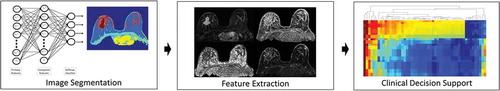
By incorporating these computational methods, future radiology reading rooms will form a unique collaboration between computer scientists and radiologists (human experts). This collaboration will enable algorithms to assist radiologists in various aspects of radiological decision making, such as, identification, segmentation, characterization of different tissue types, and prioritizing diagnosis. For example, large imaging data sets, such as brain, chest, abdomen, pelvis and breast could be quickly triaged into different groups by using deep learning methods, where the potential ‘worse’ cases are looked at first by a radiologist, leading to increased efficacy and confidence of the radiologist. Other data mining methods using machine learning can be further developed to integrate radiological parameters with other information extracted from different sources such as pathology and clinical history using electronic health records [14–17]. The integration of these data types, will give clinicians a more complete picture of the state of health in the patient, help with a more accurate diagnosis, and improved understanding of the complex nature of the disease. When the data is taken together, personalized treatment planning and precision disease prognosis can be achieved as shown in Figure 1. The goal of computational radiology is to extract all the qualitive and quantitative information within images and develop potential non-invasive biomarkers for detection and characterization of a disease in patients. Deep learning and radiomics are emerging areas in computational radiology that fulfil this goal.

Figure 1. Conceptual computational radiology framework for personalized radiological diagnosis and prognosis. There are three major components of the proposed framework – image segmentation, feature extraction and integrated clinical decision support model.

Deep learning is a renewed area of research that deals with development of deep artificial neural networks that were inspired by biological neural networks in our brain [4,6,18–42]. In radiology, deep neural networks, like biological neural networks, attempt to learn an intrinsic representation of the radiological data, for example, where in MRI, fluid is dark on a T1-weighted sequence and bright on T2-weighted sequence. This information can train a deep learning algorithm to recognize patterns and perform accurate segmentations. Deep learning has produced excellent results in a variety of fields, such as. object detection and recognition, text generation, music composition, and autonomous driving to name a few [1,2,43–49]. Deep learning has become an active area of research in the field of computer assisted clinical and radiological decision support in the recent years, with some excellent initial results and recently surveyed [8,9,46].

Radiomics are textural mathematical constructs that capture the spatial appearance of the tissue of interest (shape and texture) on different types of images using texture [10–13,50–53]. The texture features have been correlated to tissue biology in certain applications and recently reviewed [54]. Traditionally, radiomic features provide information about the grey-scale patterns, interpixel relationships, shape, and spectral properties within regions of interest on radiological images [50–53,55,56].

One of the major hurdles for successful translation of radiomics or deep learning algorithms from research to clinical practice in precision medicine is their interpretability. For example, in radiomics, if an entropy (first order, which is a measure of heterogeneity/disorder) or grey level cooccurrence matrix (GLCM) entropy (A higher order measure of heterogeneity/disorder based on the grey level relationship to each other in certain neighbourhoods) feature is measured as 6.5 and if there is no control or normal tissue entropy values for these metrics, it would be difficult to attach a biological meaning attached to that entropy value. The same value of the radiomic metric could mean that the underlying tissue is homogeneous or heterogeneous depending on the number of bins chosen, size of the ROI, and other pre-processing steps such as image filtering, which have an impact on the values (see below).

Similarly, since deep learning is essentially a ‘blackbox’, when the method segments and predicts the underlying tissue as either malignant or benign, deep learning does not provide an explanation behind its prediction. The physician’s interpretability would be based on the algorithm and whether, they would ‘trust’ the results, which is currently the major challenge.

This article reviews the techniques of radiomics and deep learning, outlining the current state of-the-art algorithms for application to precision medicine, their limitations, and provides an outlook on the potential future of these two techniques in precision medicine.

2. Deep learning

Deep learning techniques have gained renewed popularity in recent years with the development of advanced optimization techniques and an increase in computational efficiency. Deep learning has begun to play an integral part in many different aspects of modern society and has produced seemly excellent results in a variety of fields, such as, object detection and recognition, text generation, music composition, and autonomous driving to name a few [2,43–46,48,49]. Advanced deep learning will have an impact in precision medicine in the near future using computer assisted clinical and radiological decision support. These methods will outline new ways for training, testing, and validation of clinical tests for better integration of medicine information and provide a new visualization tool for diagnostics. We will focus on an overview and the current state of the art in deep learning methods.

Historically, deep learning methods are a subset of machine learning algorithms in computer science. Briefly, the goal of machine learning is to learn features and transform these features into class labels for segmentation or classification. Machine learning algorithms are either supervised or unsupervised and linear or non-linear in nature [57]. The major difference between deep learning and conventional machine learning algorithms lies in the fact that deep learning algorithms do not require an intermediate feature extraction or engineering step in order to learn the relationship between the input x (e.g. grey level intensity values on radiological images) and the corresponding labels y (e.g. the tissue type corresponding to these intensity values).

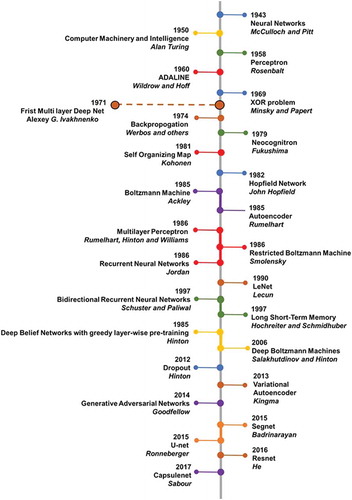
Conceptually, machine learning algorithms model the relationship between the input x and labels y using a probability distribution, p over x and y, learning algorithms, in general, can be broadly classified into generative and discriminative methods depending on p [57,58]. Generative models learn the joint probability distribution (x, y) in order to estimate the posterior probability p(y|x). Some examples of generative deep learning algorithms include generative adversarial network, variational autoencoder and deep belief networks [40,59]. In contrast, discriminative models estimate the posterior probability p(y|x) directly without calculating the intermediate joint probability distribution. In other words, discriminative models learn a direct mapping between x and y. Convolutional neural networks, stacked autoencoders, and multilayer perceptron are typical examples of discriminative deep learning algorithms [45,46]. If the problem requires us to only predict the labels y from x, then discriminative models maybe a better choice, since they are not concerned with modelling of (x, y) and more effectively model parameters to P(y|x), thereby producing a classifier with higher accuracy. However, discriminative models may not be used if the input, x consists of a large number of missing values or data points and would require data imputation. In addition, generative models allow for the generation of new synthetic data and model different relationships within the input data. For example, if the goal is to classify a lesion as benign or malignant, discriminative deep learning maybe a better choice. Whereas, if our goal is to identify intrinsic characteristics of a lesion and model their distribution across the patient population, a better choice of algorithm maybe one of the generative deep learning algorithms. The commonly used discriminative and generative deep learning algorithms for application to precision medicine are discussed below. Figure 2 provides a brief history and a timeline of major advances in the field of deep learning.

Figure 2. The timeline of major advancements in the field of deep learning.

2.1. Types of deep neural networks

2.1.1. Discriminative deep learning models

2.1.1.1. Convolutional neural networks

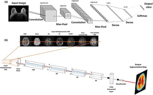
Convolutional neural networks (CNN) are the most popular neural network architectures applied to computer vision applications [27]. This is probably due to the access to available software, such as, Tensorflow, pyTorch, Matlab Deep Learning, Keras, and others. The architecture of CNNs is inspired by the hierarchical organization of visual cortex [2,29]. CNNs use local connections and weights to analyze the 2D structure of the input data (e.g. images), followed by pooling operations (e.g. max pooling) to obtain spatial invariant features. In addition, CNNs have significantly fewer trainable parameters than the corresponding fully connected networks of the same size. Typical CNN architectures are illustrated in Figure 3.

Figure 3. Illustration of convolutional neural architecture (CNN) architecture for classification of a radiological image for clinical diagnosis. (a) The CNN architecture shown here consists of two convolutional layers (each followed by a max-pooling layer), followed by two fully connected (dense) layers for image classification. (b) An example of a patch-based CNN applied to a multiparametric brain MRI dataset for segmentation of the different brain tissue types.

The conventional CNN architecture has been modified and extended to encompass different architectures to improve the state-of-the-art results for applications in computer vision and other domains. Some of the most notable architectures for the task of classification or object recognition include Alexnet [2], Resnet [6], Densenet [7], and Inception [3]. The comparison of different deep learning architectures based on their performance, amount of single pass operations, and the number of network parameters has been detailed in [60]. The current state-of-the art CNN techniques for semantic (coarse to fine) segmentation include Segnet [4], U-net [5], and their variants.

2.1.1.2. Stacked autoencoders

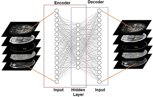
Autoencoders are a class of unsupervised neural networks that learn intrinsic representations of their input data by attempting to reconstruct it [33]. As a result, autoencoders transform the input data into a compact or a low dimensional representation of its intrinsic dimensionality. For supervised learning tasks, Autoencoders are especially useful when the input data has a large number of unlabelled examples compared to labelled examples or the data is sparse in regard to training [61,62]. A typical architecture for autoencoders is illustrated in Figure 4.

Figure 4. Illustration of an autoencoder used to learn a low dimensional representation of the high dimensional multiparametric MRI brain dataset by attempting to reconstruct it.

Some of the typical applications of autoencoders include representation learning (e.g. Sparse Autoencoders), classification (e.g. Stacked Sparse Autoencoders), and image denoising (e.g. Stacked Denoising Autoencoders [61]). Furthermore, autoencoders have also been extended to develop generative neural network model known as Variational Autoencoder [39]. This is done by modifying the encoder such that it generates latent vectors that roughly follow a unit gaussian distribution. The constraint is enforced by changing the loss function to include both, the mean squared error between the input and the output and the Kullback-Leibler (KL) divergence between the latent vector and unit gaussian distribution. Variational autoencoders have begun to find applications in unsupervised and semi-supervised feature extraction and segmentation [63–65].

2.1.2. Generative deep learning models

2.1.2.1. Deep belief network

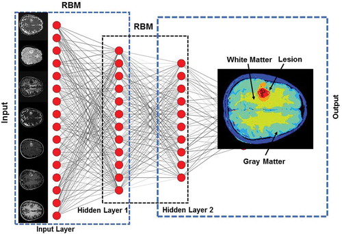
Deep Belief Networks (DBNs) are a class of generative deep neural networks that are composed of multiple layers of stochastic, latent variables [66]. Each layer of the DBN acts as a hidden layer for the previous layer and input layer for the subsequent layer. In addition, there are no connections between the nodes within each layer. Each layer of DBN can be viewed as an unsupervised network such as Restricted Boltzmann Machine (RBM) [34] or an Autoencoder [33], which is trained in a greedy unsupervised fashion utilizing the outputs from the previous layer. Figure 5 illustrates the architecture of a typical DBN.

Figure 5. Illustration of a Deep Belief Network (DBN) with two hidden layers for segmentation of an example multiparametric MRI brain dataset. Each layer is pre-trained in an unsupervised fashion using Restricted Boltzmann Machines (RBMs) utilizing the outputs from the previous layer. The output from DBN segmentation on the example dataset is shown in the output layer.

2.1.2.2. Generative adversarial network

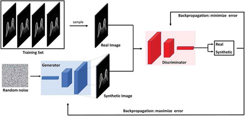
Generative Adversarial Networks (GANs) are currently the most popular generative deep learning architectures [40]. GANs consists of two neural network architectures competing against each other in a zero-sum game framework. One network generates candidates (generator) while the other evaluates them (discriminator). The goal of the generator is to synthesize realistic instances from the input data distribution while the goal of the discriminator is to differentiate between the true and synthesized instances of the input data distribution. The training objective of the generator is to maximize the error rate of the discriminator, which is approximately 50% [40,67]. Once trained, the generator learns to map from a latent space to the input data distribution. Figure 6 illustrates the architecture of a typical GAN. The major application of GANs has been image, video and speech synthesis [68–73]. In medical image analysis, GANs have been used in medical image synthesis, segmentation, registration, and data augmentation. A detailed review of GANs and their application to medical image analysis can be found in [67].

Figure 6. Illustration of the generative adversarial network (GAN) architecture. GANs consists of two neural network architectures competing against each other in a zero-sum game framework. One network generates candidates (generator) while the other evaluates them (discriminator). The goal of the generator is to synthesize realistic instances from the input data distribution while the goal of the discriminator is to differentiate between the true and synthesized instances of the input data distribution.

2.1.3. Deep reinforcement learning

Historically, reinforcement learning (RL) is a multifaceted area of research where the RL algorithm attempts learning actions to optimize some type of action(s) in a defined state(s) and weight any tradeoffs for most maximal reward(s) possible [74,75]. The main elements required for RL are a policy, reward signal, value function, and a model of the defined environment [75]. In depth discussion of these and other RL aspects are extensively examined in Sutton [75]. Reinforcement learning algorithms are goal-oriented algorithms that attempt to maximize a particular reward over many actions, where in, the RL algorithm is rewarded or penalized at each action on whether it takes a right or a wrong move. Finally, the action is evaluated based on its contribution to the final reward [76–85]. For example, finding the right combination of moves to get the largest amount of points and win.

Deep reinforcement learning is a rapidly growing area rapidly growing area in the field of reinforcement learning with groundbreaking results, such as speech recognition [86], playing Atari [87] and AlphaGo [88]. In deep reinforcement learning, deep learning algorithms are trained to identify the current state and predict the next best move (e.g. a CNN can be trained to capture the computer screen of a game as the current state, and then predict which button to press on the keyboard to maximize the final score in the game) [87].

Deep reinforcement learning algorithms have begun to find applications in landmark detection and treatment response prediction in the field of computational radiology [83–85]. In landmark detection, deep reinforcement learning is used to search for a landmark (e.g. pancreas) in the body, making it faster than the standard search algorithms [85]. In treatment response assessment, deep reinforcement learning algorithms can be trained to predict the effect of a drug on patient’s treatment and whether they will respond to treatment or not [83].

2.2. Deep neural networks – looking under the hood

One of the major hurdles for successful translation of deep learning algorithms from research to practice in precision medicine is their interpretability. A large number of studies have shown that deep neural networks can be easily fooled [89–92], which makes their interpretability even more important for radiological applications.

Deep neural networks are like a black box. i.e. we don’t know how the deep neural networks organize, integrate and interpret the imaging information. For example, when radiologists develop an intrinsic representation of ‘fat’ in their brain, they store it as ‘bright on T1 and dark on T2’. Similarly, an intrinsic representation of ‘fluid’ would be stored as ‘dark on T1 and bright on T2’. The main question here is ‘How do deep neural networks encode the input intrinsic representations?’.

In the recent years, a large number of studies have attempted to open the deep learning black box, with excellent results, with Activation Maximization [93], Deconvolutional Network [94], Network Inversion [95], and Network Dissection [96] comprising the major techniques developed to improve network interpretability. A detailed review of these techniques can be found in [97]. Here, we will provide an overview of these techniques in the following subsections.

2.2.1. Activation maximization

The idea behind activation maximization is to identify input patterns that maximize the activation of a particular neuron. By identifying the optimal set of input patterns for different neurons in the network, it would be possible to decode what these neurons represent in terms of the input space. As an example, for a network trained to recognize faces, the method of activation maximization would be useful in identifying neurons that specialize in recognizing different facial features such as nose, eyes, and mouth. The interpretability of the visualization of input patterns using activation maximization have received significant interest in the recent years leading to improved algorithms [98].

2.2.2. Deconvolutional network

Deconvolutional networks interprets the convolutional networks from the point of view of the input image, as opposed to individual neurons for activation maximization [94,99,100]. Deconvolutional networks highlight the patterns of the input image that activate individual neurons in each layer, providing a tool to interpret the network and identify any problems with the trained network.

2.2.3. Network inversion

The techniques of activation maximization and deconvolutional networks were concerned with interpreting the network from a neuronal perspective. On the other hand, network inversion attempts to analyze the activation pattern from the perspective of a layer. Network inversion, as the name suggests, attempts to reconstruct the input from an arbitrary layer’s activation patterns [95]. Network inversion provides a tool to interpret the information a specific layer would store. In recent years, many different methods for network inversion have been proposed such as Hoggles [101] and up-convolutional neural networks [102] that are capable of reconstructing inputs from feature spaces generated by any algorithm such as Histogram of Gradients (HoG) [103], Scale Invariant Feature Transform (SIFT) [104], or convolutional neural networks [27].

2.2.4. Network dissection

The techniques of activation maximization, deconvolutional networks, and network inversion provided tools to understand the activation patterns of a specific neuron or a layer. However, these methods do not provide a semantic interpretation of these activation patterns. Consequently, Bau et al. [96] proposed the technique of network dissection, which attempts to associate every neuron in the convolutional neural network with a semantic concept.

3. Radiomics

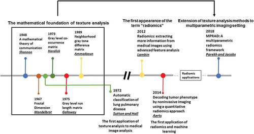
Radiomics has been widely applied to many different precision medicine applications across different organs and modalities. Recent reviews on the mathematical background and applications of radiomics can be found in [54] with limitations of radiomics discussed in [105]. The current state-of-the art techniques in radiomics deal with extraction of first and higher order statistical features from radiological images [50–53,55,56]. We will overview some of the newer advancements in the field of radiomics followed by a detailed discussion on the interpretability of radiomics in the following subsections. A brief history of radiomics has been illustrated in Figure 7.

Figure 7. The timeline of important advancements in the field of texture and radiomics.

3.1. Multiparametric radiomics

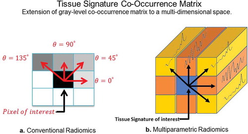
Traditionally, radiomics was developed for extraction of features from a single modality (e.g. CT scans on patients with lung cancer). The field of radiomics is rapidly expanding towards application to a multiparametric imaging setting, where multiple different imaging sequences are acquired on a patient for a more complete diagnosis. As a result, novel multiparametric radiomic (MPRAD) methods were recently developed to integrate all the imaging information present within the multiparametric data set resulting in new metrics of radiomic features [106]. The MPRAD features were based on the extraction of inter-tissue-signature relationships in high dimensional multiparametric imaging data, as opposed to the inter-voxel relationships extracted by conventional radiomic features in single images or regions of interest, as illustrated in Figure 8. The MPRAD allows for better tissue delineation between tissue types and allows for improves quantitative radiomic measures for diagnostic use in precision medicine.

Figure 8. Illustration of the differences between GLCM radiomic features from conventional single image and multiparametric radiomics. (a). Single image radiomics features extract the inter-pixel relationships in-plane of a radiological image whereas, (b). the multiparametric radiomics extract the inter-tissue-signature relationships across multiple radiological images.

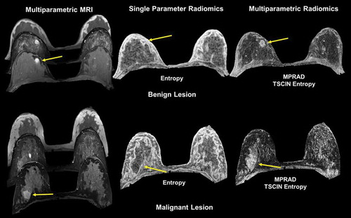
Multiparametric radiomics on breast lesions have resulted in higher classification between malignant and benign breast lesions with a sensitivity and specificity of 82.5% and 80.5% with an AUC of 0.87 [106]. More importantly, using multiparametric radiomics, there was an increase of 9%-28% in the AUC over single radiomic methods. In brain patients with acute stroke, multiparametric radiomics were able to distinguish the perfusion-diffusion mismatch more completely than single parameter radiomics [106]. Figure 9 illustrates the use of multiparametric radiomics on both a benign and malignant lesion.

Figure 9. Illustration of multiparametric radiomic feature maps obtained from single and multiparametric radiomic analysis in a benign and malignant lesion. Top Row: Example of a patient with a benign lesion, where the straight yellow arrow highlights the lesion. There are clear differences between the single and multiparametric entropy radiomic images, where the multiparametric clearly demarcates the lesion. Bottom Row: Similar analysis on a patient with a malignant lesion (yellow arrow). Again, the multiparametric entropy map improves tissue delineation between the glandular and lesion tissue.

3.2. Interpretability of radiomics

Interpretability of radiomic features has been a major limitation of radiomics since its inception. This is partly because the radiomic features are not standardized and the difficulty relating to the underlying biology of the tissue of interest. For example, radiomic features extracted from a region of interest (ROI) are dependent on the size of the ROI and the number of grey levels and bins selected for image quantization as detailed in the following subsections.

3.2.1. Dependence on the size of ROI

Consider the first order features of entropy and uniformity, given by the following equations:

(1) $Entropy=-{\mathrm{\Sigma }}_{i=1}^{B}H(i){log}_{2}H(i)$(1)

and

(2) $Uniformity={\mathrm{\Sigma }}_{i=1}^{B}H(i{)}^2$(2)

Here, H is the first order histogram with B number of bins.

The range of values that the first order entropy feature can take varies between 0 and log₂ N, where N is the number of voxels in the tissue. Similarly, the range of values that the uniformity feature can take varies between (1/N) and one. For example, consider a 5 × 5 sized ROI. The minimum heterogeneity or maximum uniformity for this ROI occurs when all the voxels have the same intensity value. In this case, the value of (1) = 1 and H(i) = 0 for all i ∈ {2,3, …, B}. Consequently, the entropy and uniformity values for this ROI are 0 and 1, respectively. But, the maximum heterogeneity or minimum uniformity occurs when all the voxels have different intensity values. In this case, the value of (i) =$\frac{1}{25}$for all i ∊ {1,2, …, B}. As a result, the entropy and uniformity value for this ROI are log₂ 25 = 4.64 and 0.04, respectively.

The dependence between the size of the ROI and radiomic features has been observed in a large number of studies and reviewed in [105]. There are two potential methods for overcoming this limitation: radiomic feature mapping and feature normalization.

Radiomic feature mapping (RFM) transforms radiological images into texture images using statistical kernels based on first and second order statistics [13]. The RFM computes a radiomic value for every voxel in the radiological image, thereby negating the effect of size dependence. However, computation of RFMs has a high time complexity. For second order GLCM features, the time complexity for computing RFM using a W × W sized sliding window is O(N²,G²,W²) for an N × N radiological image quantized to G gray levels. Recently, using deep convolutional neural networks were preliminarily successful in synthesizing entropy feature maps in MRI breast cancer studies [107].

The radiomic features can also be normalized to the size of the ROI. For example, the equation for computing first order entropy can be modified to

(3) $Entropy=-\frac{({\mathrm{\Sigma }}_{i=1}^{B}H(i)lo{g}_{2}H(i))}{{log}_{2}N}$(3)

where N represents the number of voxels in the ROI.

Recently, Shafiq-ul-Hasan et al. [108] extended this measure for feature normalization by voxelsize across all the features and demonstrated their technique in limited CT lung cancer studies [109].

In the future, these methods need to be validated across multiple modalities and organs.

4. Dependence on the image binning and gray level quantization

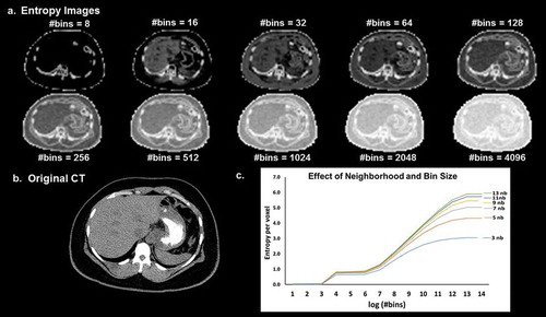
There is an inherent dependence between the number of gray levels or bins used for radiomic analysis and the corresponding radiomics features. This dependence can be seen from Equations (1) and (2) where the number of bins is used as an input variable for the computation of entropy and uniformity. Figure 10 demonstrates the dependence of entropy on binning and the neighbourhood parameter used for image filtering. When there is an increase in binning, it leads to loss of information and image contrast.

Figure 10. (a). Illustration of the dependence of the entropy value from the neighborhood size used for image filtering and image binning on a (b). CT image (Soft tissue window). (c). The curves of entropy vs bins appear to follow a distinct pattern where in the entropy values vary linearly with the log of number of bins within a certain range and remain more or less constant outside that range. The value of the entropy consistently increases with the increase in the size of the neighborhood filter.

The dependence between grey level quantization and GLCM features was evaluated by Shafiqul-Hasan et al. [108] for certain second order features. The authors found that the radiomic features had either linear, quadratic, or cubic relationship with the number of grey levels for the selected set of features. The authors further proposed modified equations for computation of different radiomic features and tested their efficacy on different phantoms. However, grey level quantization actually changes the information present in the radiological images. Apart from mathematical dependence, there is also an intrinsic dependence between gray level quantization and radiomic features, which has not yet been addressed in any study. For example, if we consider an extreme case of quantization of a radiological image to one gray level, we would lose all the information present in the image.

This information loss in radiological images cannot be corrected by mathematically modifying the radiomic formula, but by selecting an optimal number of gray levels. Currently, no standardized method exists for the selection of number of gray levels that would minimize the loss of information in the resultant quantized image. In the future, standardization of radiomics would only be possible by standardizing the procedure for selection of the optimal gray level or a range of ideal gray levels for quantization of radiological images for use across multiple platforms.

5. Discussion

Deep learning and radiomics methods are influencing a paradigm shift in precision radiology research In the recent years, deep learning methods have found applications in many research areas of medical image analysis, ranging from image acquisition to image registration, segmentation, and classification [8,9]. Radiomics has provided a new quantitative metric based on the texture of the gray levels in the image to assist in detection and characterization of different pathologies. By combining radiomics and deep learning together, they have the potential to completely revolutionize the field of radiology and usher in a new area of personalized imaging medicine [107].

The current state-of-the-art techniques in radiomics face some challenges in terms of interpretability, standardization, and visualization. The preprocessing step of gray level quantization is an active area of research in radiomics. This quantization of the image could potentially alter the intrinsic information present in the radiological image. These changes in the radiological images cannot be mathematically corrected and may produce incorrect results in terms of texture features. In the future, quantitative radiomic metrics need to be developed that are similar to signal-to-noise and contrast-tonoise ratios, which would to measure the information loss between the original and quantized radiological images. In addition, a standardized tolerance level would need to be defined to ensure correctness of radiomic results. Finally, there is active research in linking the texture features to the biology of the tissue of interest. This link to biology may be accelerated with the introduction of multiparametric radiomics, where multiple images with known biology properties can be related directly to the texture features. Whereas, in the past, only single images could be used.

Recent reports have shown that deep learning methods, particularly CNN, are capable of capturing the textural information present in the radiological images in the initial convolutional layers. This textural information could be visualized using advanced techniques for network interpretability to better understand the meaning of different radiomic methods. For example, visualizing the difference in the texture feature for images with low versus high entropy values would be very informative for heterogeneity of a tissue. In addition, CNNs could potentially completely replace current methods for generating radiomic data from radiological images as shown by preliminary work in this direction [107]. Deep learning methods have shown excellent success in computer vision research with the development of novel architectures such as Resnet [6], Densenet [7], and Inception [3]. However, these architectures are optimized for application to computer vision (e.g. Imagenet) for red, green, and blue images and may not be optimized for application to medical image analysis, where, they are based in a gray level scale. The direct translation of these architectures to the medical domain may not produce optimal results, especially for multiparametric and multimodal imaging datasets. Domain knowledge about the underlying task could provide the essential bridge for translating these deep learning architectures for application to medical imaging methods. Some initial translation has been shown from Kaggle in the diabetic retinopathy challenge based on optical imaging [110]. There are two major components in a typical deep learning framework where domain knowledge could improve the efficacy of deep learning in medical image analysis. The first component deals with image pre-processing (e.g. normalization) prior to training deep neural networks. Many applications have demonstrated that scale standardization is essential for training and testing machine and deep learning algorithms [111,112].

The second component is the neural network architecture itself. A typical example of a deep learning architecture developed for the specific task of semantic segmentation is U-net [5].

The translation from vision to medical image analysis applications presents some unique challenges. For example, the segmentation or classification problem is normally formulated as a binary problem, where in, the heterogeneity within the normal or abnormal tissue is not evaluated. This problem can be potentially resolved by annotating all possible classes within each tissue type. However, this solution is both impractical and computationally expensive as it would require experts to carefully annotate each image with all possible tissue classes. As a result, unsupervised deep learning approaches such as Autoencoders [33], Generative Adversarial Networks [40], or Deep Belief Networks [66] could be applied to characterize the underlying tissue heterogeneity.

Deep learning methods currently face some challenges, such as, interpretability, optimization, and validation (in a prospective sense). There have been major advances with the development of algorithms that could potentially open the deep learning ‘black box’ for a number of deep neural networks. These techniques include Activation Maximization [93], Deconvolutional Network [94], Network Inversion [95], and Network Dissection [96]. The techniques of activation maximization and deconvolutional network deal with the network interpretation from a neuronal perspective, network inversion attempts to reconstruct the input from the network’s point of view, and network dissection associates every neuron in the convolutional neural network with a semantic concept. Recently, a novel interface was proposed by combining the existing techniques for interpreting deep neural networks and treating them as fundamental and composable building blocks for such interfaces [113]. However, these methods are yet to be translated to clinical and radiological data for application to precision medicine. In the future, we will see these techniques being translated to understand algorithms developed for analyzing clinical and radiological data in addition to newer specialized techniques developed specifically for understanding such datasets. In addition, some deep learning models are easily fooled by introduction of adversarial patches [92]. Recently, newer architectures are being developed to produce deep networks resilient to adversarial attacks [114].

Optimization of the deep neural network architecture presents a significant challenge. The search space of network parameters is generally very big and maybe impractical to empirically evaluate the complete search space to develop the optimal neural network architecture for a specific task. For this purpose, newer methods are being developed to efficiently compute optimal neural network architectures (e.g. Adanet [115]). Adanet adaptively optimizes both the structure of the network and the weights for each connection. Furthermore, the deep networks trained with or without advanced optimization algorithms such as Adanet are still trained at one particular point in time with a limited sized dataset. The neural networks should be able to automatically update their architecture as they encounter more data (similar to human brain). This type of network is referred to as life-long learning and recently reviewed describing several different methods proposed in the literature for life-long learning [116]. In the future, deep learning methods for clinical decision support system would not just be a single neural network but a hybrid framework incorporating algorithms for decision support, network interpretability, network optimization and life-long learning.

In conclusion, both deep learning and radiomics are two rapidly advancing technologies that may unite in the future to produce a single unified framework for clinical decision support with a potential to completely revolutionize the field of precision medicine.

Deep learning and radiomics are rapidly taking over in many areas of research and is a relatively new field of research, even though it uses methods developed decades ago. The embrace of deep learning has been in the development of economical and increased computational methods with early success in many different areas. However, extensive research is required to evaluate how the network is working at each layer and the transfer of the weights into the nodes. Optimization of network hyperparameters, such as, batch normalization, regularization, fitting parameters, etc., Similarly, for radiomics, the major challenge is the link to biology and function. There are several major steps that need to be addressed, such as. preprocessing steps such as quantization, optimal methods for data gray level and binning, as well as optimal neighborhood sizes for different image resolutions. Establishing the standards for both of these methods will require more research along with validation studies.

In the next five years, we will witness deep learning and radiomic methods transform medical imaging and its application to personalized medicine. These techniques will evolve to hybrid systems based on combinations of the different networks and advanced radiomic methods for a more complete diagnosis.

In conclusion, as deep learning and radiomics methods mature, their use will become part of clinical decision support systems and can be used to rapidly mine patient data spaces and radiological imaging biomarkers to move medicine towards the goal of precision medicine for patients.

Article highlights

• Deep Learning and Radiomics are creating a paradigm shift in radiology and precision medicine by developing a new area of research to be used for precision medicine.

• Development and identification of biological correlation to deep learning features and networks are needed for wide spread implementation of deep learning in precision medicine.

• Development and identification of biological correlation to radiomics features are needed for wide spread implementation of radiomics in precision medicine.

• Further research is needed to determine the optimal processing steps needed for reproducible application of deep learning to different imaging applications, for example, imaging modality, optimization of hyperparameters, network size, and type of network (CNN, SAE, etc) just to name a few.

• One of the major hurdles for successful translation of deep learning algorithms from research to practice in precision medicine is their interpretability to physicians.

• Prospective trials and follow up studies are needed to fully define the impact of deep learning and radiomics for diagnosis and precision medicine in patients.

Author contributions

VSP and MAJ developed the concept, performed the literature research, and manuscript writing

Declaration of interest

The authors have no other relevant affiliations or financial involvement with any organization or entity with a financial interest in or financial conflict with the subject matter or materials discussed in the manuscript apart from those disclosed.

Reviewer disclosures

Peer reviewers on this manuscript have no relevant financial or other relationships to disclose.

Additional information

Funding

Funding provided by the National Institutes of Health (NIH) grant numbers: 5P30CA006973 (Imaging Response Assessment Team-IRAT), U01CA140204, 1R01CA190299, and The Tesla K40s used for this research was donated by the NVIDIA Corporation.

References

- Ciresan DC, Meier U, Masci J, et al. Flexible, high performance convolutional neural networks for image classification. Proc Twenty-Second Int joint Conf on Artif Intell. 2011;2: 1237–1242.
- Krizhevsky A, Sutskever I, Hinton GE. Imagenet classification with deep convolutional neural networks. Adv Neural Inf Process Syst. 2012;1097–1105.
- Szegedy C, Liu W, Jia Y, et al. Going deeper with convolutions. Comput Vision Pattern Recognit. 2015;1–9.
- Badrinarayanan V, Kendall A, Cipolla R. Segnet: a deep convolutional encoder-decoder architecture for image segmentation. arXiv:151100561. 2015:1–14.
- Ronneberger O, Fischer P, Brox T U-net: convolutional networks for biomedical image segmentation. International Conference on Medical image computing and computer-assisted intervention. 2015. p. 234–241.
- He K, Zhang X, Ren S, et al. Deep residual learning for image recognition. Comput Vision Pattern Recognit. 2016;770–778.
- Huang G, Liu Z, Van Der Maaten L, et al. Densely connected convolutional networks. Comput Vision Pattern Recognit. 2017;1(2):4700–4708.
- Litjens G, Kooi T, Bejnordi BE, et al. A survey on deep learning in medical image analysis. Med Image Anal. 2017;42:60–88.
- Cao C, Liu F, Tan H, et al. Deep learning and its applications in biomedicine. Genomics Proteomics Bioinformatics. 2018.
- Kumar V, Gu Y, Basu S, et al. Radiomics: the process and the challenges. Magn Reson Imaging. 2012 Nov;30(9):1234–1248.
- Lambin P, Rios-Velazquez E, Leijenaar R, et al. Radiomics: extracting more information from medical images using advanced feature analysis. Eur J Cancer. 2012;48(4):441446.
- Aerts HJ, Velazquez ER, Leijenaar RT, et al. Decoding tumour phenotype by noninvasive imaging using a quantitative radiomics approach. Nat Commun. 2014;5:4006.
- Parekh VS, Jacobs MA. Integrated radiomic framework for breast cancer and tumor biology using advanced machine learning and multiparametric MRI. NPJ Breast Cancer. 2017;3(1):43.
- Amarasingham R, Moore BJ, Tabak YP, et al. An automated model to identify heart failure patients at risk for 30-day readmission or death using electronic medical record data. Med Care. 2010 Nov;48(11):981–988.
- Masanz JJ, Ogren PV, Jiaping Z, et al. Mayo clinical text analysis and knowledge extraction system (cTAKES): architecture, component evaluation and applications. J Am Med Inf Assoc. 2010;17(5):507–513.
- Hayes MG, Rasmussen-Torvik L, Pacheco JA, et al. Use of diverse electronic medical record systems to identify genetic risk for type 2 diabetes within a genome-wide association study. J Am Med Inf Assoc. 2012;19(2):212–218.
- Choi S, Ivkin N, Braverman V, et al. DreamNLP: novel NLP system for clinical report metadata extraction using count sketch data streaming algorithm: preliminary results. arXiv:180902665. 2018:1–13.
- McCulloch WS, Pitts W. A logical calculus of the ideas immanent in nervous activity. Bull Math Biophys. 1943;5(4):115–133.
- Turing A. Computer Machinery and Intelligence. Mind. 1950;LIX(236):433–460.
- Farley B, Clark W. Simulation of self-organizing systems by digital computer. Trans IRE Prof Group Inf Theory. 1954;4(4):76–84.
- Rosenblatt F. The perceptron: A probabilistic model for information storage and organization in the brain. Psychol Rev. 1958;65(6):386–408.
- Widrow B, Hoff ME. Adaptive switching circuits. IRE WESCON Convention Rec. 1960;4:96104.
- Ivakhnenko AG, Lapa VG. Cybernetic predicting devices. CCM Information Corp. 1966;1–255.
- Minsky M, Papert S. Perceptrons: an introduction to computational geometry. Cambridge (MA): MIT Press; 1969.
- Ivakhnenko AG. Polynomial Theory of Complex Systems. IEEE Trans Syst Man Cybern Syst. 1971;1(4):364–378.
- Werbos P. Beyond regression: new tools for prediction and analysis in the behavioral sciences [Ph D dissertation]. Harvard University; 1974.
- Fukushima K. Neural network model for a mechanism of pattern recognition unaffected by shift in position-Neocognitron. IEICE Tech Rep A. 1979;62(10):658–665.
- Eigen M. Selforganization in molecular and cellular networks. Neurochem Int. 1980;2C:25.
- Fukushima K. Neocognitron: A self-organizing neural network model for a mechanism of pattern recognition unaffected by shift in position [journal article]. Biol Cybern. 1980;36(4):193–202.
- Kohonen T Automatic formation of topological maps of patterns in a self-organizing system. Proc 2nd Scand Conf on Image Analysis. 1981. p. 214–220.
- Hopfield JJ. Neural networks and physical systems with emergent collective computational abilities. Proc Natl Acad Sci U S A. 1982 Apr;79(8):2554–2558.
- Ackley DH, Hinton GE, Sejnowski TJ. A learning algorithm for Boltzmann machines. Cognit Sci. 1985;9(1):147–169.
- Rumelhart DE, Hinton GE, Williams RJ. Learning internal representations by error propagation. La Jolla: Univ California San Diego - Institute for Cognitive Science; 1985. p. 1–49.
- Smolensky P. Information processing in dynamical systems: foundations of harmony theory; CU-CS-321-86; 1986. (Computer Science Technical Reports: Colorado Univ At Boulder Dept Of Computer Science). p. 1–56.
- LeCun Y, Boser BE, Denker JS, et al. Handwritten digit recognition with a back-propagation network. Adv Neural Inf Process Syst. 1990;396–404.
- Hochreiter S, Schmidhuber J. Long short-term memory. Neural Comput. 1997 Nov 15;9(8):1735–1780.
- Schuster M, Paliwal KK. Bidirectional recurrent neural networks. IEEE Trans Signal Process. 1997;45(11):2673–2681.
- Hinton GE, Srivastava N, Krizhevsky A, et al. Improving neural networks by preventing coadaptation of feature detectors. arXiv:12070580. 2012:1–18.
- Kingma DP, Welling M. Auto-encoding variational bayes. arXiv:13126114. 2013:1–14.
- Goodfellow I, Pouget-Abadie J, Mirza M, et al. Generative adversarial nets. Adv Neural Inf Process Syst. 2014;2672–2680.
- Ronneberger O, Fischer P, Brox T. U-Net: convolutional networks for biomedical image segmentation. arXiv:150504597. 2015:1–8.
- Sabour S, Frosst N, Hinton GE. Dynamic routing between capsules. Adv Neural Inf Process Syst. 2017;3856–3866.
- Deng J, Dong W, Socher R, et al. Imagenet: A large-scale hierarchical image database. Comput Vision Pattern Recognit. 2009;248–255.
- Gatys LA, Ecker AS, Bethge M. Image style transfer using convolutional neural networks. Comput Vision Pattern Recognit. 2016;2414–2423.
- LeCun Y, Bengio Y, Hinton G. Deep learning. Nature. 2015;521(7553):436–444.
- Schmidhuber J. Deep learning in neural networks: an overview. Neural Networks. 2015 [cited 2015 Jan 01];61:85–117.
- Goodfellow I, Bengio Y, Courville A, et al. Deep learning. MIT press Cambridge; 2016.
- Briot J-P, Hadjeres G, Pachet F. Deep learning techniques for music generation-a survey. arXiv:170901620. 2017:1–189.
- Xu HZ, Gao Y, Yu F, et al. End-to-end learning of driving models from large-scale video datasets. Comput Vision Pattern Recognit. 2017;3530–3538.
- Shannon CE. A mathematical theory of communication. Bell Syst Techn J. 1948 July;27(3):379–423.
- Haralick RM, Shanmugam K, Dinstein IH. Textural features for image classification. IEEE Trans Syst Man Cybern Syst. 1973;6:610–621.
- Galloway MM. Texture analysis using gray level run lengths. Comput Graphics Image Process. 1975 [cited 1975 June 01];4(2):172–179.
- Laws KI Rapid texture identification. Proceedings of SPIE 0238, Image Processing for Missile Guidance. 1980. p. 376–381.
- Parekh V, Jacobs MA. Radiomics: a new application from established techniques. Expert Rev Precis Med Drug Dev. 2016 [cited 2016 March 03];1(2):207–226.
- Mandelbrot BB. The fractal geometry of nature. Vol. 173. Macmillan; 1983.
- Amadasun M, King R. Textural features corresponding to textural properties. IEEE Trans Syst Man Cybern Syst. 1989;19(5):1264–1274.
- Alpaydin E. Introduction to machine learning. 3rd ed. MIT press; 2014.
- Ng AY, Jordan MI. On discriminative vs. generative classifiers: A comparison of logistic regression and naive bayes. Adv Neural Inf Process Syst. 2002;841–848.
- Li C, Wand M Precomputed real-time texture synthesis with Markovian generative adversarial networks. arXiv:160404382v1. 2016:1–17.
- Canziani A, Paszke A, Culurciello E. An analysis of deep neural network models for practical applications. arXiv:160507678. 2016:1–7.
- Vincent P, Larochelle H, Lajoie I, et al. Stacked denoising autoencoders: learning useful representations in a deep network with a local denoising criterion. J Mach Learn Res. 2010;11(Dec):3371–3408.
- Parekh VS, Macura KJ, Harvey S, et al. Multiparametric deep learning tissue signatures for a radiological biomarker of breast cancer: preliminary results. arXiv:180208200. 2018:1–23.
- Hjelm RD, Plis SM, Calhoun VC. Variational autoencoders for feature detection of magnetic resonance imaging data. arXiv:160306624. 2016.
- Sedai S, Mahapatra D, Hewavitharanage S, et al. Semi-supervised segmentation of optic cup in retinal fundus images using variational autoencoder. International Conference on Medical Image Computing and Computer-Assisted Intervention. 2017. p. 75–82.
- Uzunova H, Handels H, Ehrhardt J Unsupervised pathology detection in medical images using learning-based methods. In: Bildverarbeitung für die Medizin 2018. Springer; 2018. p. 61–66.
- Hinton GE, Osindero S, Teh YW. A fast learning algorithm for deep belief nets. Neural Comput. 2006 Jul;18(7):1527–1554.
- Yi X, Walia E, Babyn P. Generative adversarial network in medical imaging: a review. arXiv:180907294. 2018.
- Mirza M, Osindero S. Conditional generative adversarial nets. arXiv:14111784. 2014:1–7.
- Radford A, Metz L, Chintala S. Unsupervised representation learning with deep convolutional generative adversarial networks. arXiv:151106434. 2015:1–16.
- Ledig C, Theis L, Huszár F, et al. Photo-realistic single image super-resolution using a generative adversarial network. Comput Vision Pattern Recognit. 2017;105–114.
- Zhang H, Xu T, Li H, et al. Stackgan: text to photo-realistic image synthesis with stacked generative adversarial networks. arXiv:161203242. 2017:1–14.
- Nie D, Trullo R, Lian J, et al. Medical image synthesis with context-aware generative adversarial networks. International Conference on Medical Image Computing and Computer-Assisted Intervention. 2017. p. 417–425.
- Zhu J-Y, Park T, Isola P, et al. Unpaired image-to-image translation using cycle-consistent adversarial networks. arXiv:170310593. 2017:1–10.
- Schmidhuber J. A local learning algorithm for dynamic feedforward and recurrent networks. Connection Sci. 1987;1(4):403–412.
- Sutton RS, Barto AG. Reinforcement Learning: an Introduction. 2nd ed. MIT Press; 2018.
- Schmidhuber J Recurrent networks adjusted by adaptive critics. Int Neural Network Conf. 1990;1:719–722.
- Schmidhuber J Reinforcement learning with interacting continually running fully recurrent networks. Int Neural Network Conf. 1990;2:817–820.
- Schmidhuber J. Reinforcement learning in Markovian and non-Markovian environments. Adv Neural Inf Process Syst. 1991;3:500–506.
- Kaelbling L, Littman M, Moore A. Reinforcement Learning: A Survey. J Artif Intell Res. 1996;4:237–285.
- Sutton RS. Temporal credit assignment in reinforcement learning. University of Massachusetts Amherst; 1984.
- Bakker B Reinforcement learning with long short-term memory. Int Conf Neural Inf Process Syst. 2001;14:1475–1482.
- Graves A, Fernández S, Schmidhuber J Reinforcement learning with interacting continually running fully recurrent networks. Int Conf Artif Neural Networks. 2007;17:549–558.
- Tseng HH, Luo Y, Cui S, et al. Deep reinforcement learning for automated radiation adaptation in lung cancer. Med Phys. 2017;44(12):6690–6705.
- Meyer P, Noblet V, Mazzara C, et al. Survey on deep learning for radiotherapy. Comput Biol Med. 2018;98(198):126–146.
- Ghesu F-C, Georgescu B, Zheng Y, et al. Multi-scale deep reinforcement learning for real-time 3D-landmark detection in CT scans. IEEE Trans Pattern Anal Mach Intell. 2019;41(1):176–189.
- Graves A, Mohamed A, Hinton G. Speech recognition with deep recurrent neural networks. arXiv:13035778. 2013:1–5.
- Mnih V, Kavukcuoglu K, Silver D, et al. Human-level control through deep reinforcement learning. Nature. 2015;518:529–533.
- Silver D, Huang A, Maddison CJ, et al. Mastering the game of Go with deep neural networks and tree search. Nature. 2016;529(7587):484.
- Nguyen A, Yosinski J, Clune J. Deep neural networks are easily fooled: high confidence predictions for unrecognizable images. Comput Vision Pattern Recognit. 2015;427–436.
- Moosavi-Dezfooli S-M, Fawzi A, Frossard P. Deepfool: a simple and accurate method to fool deep neural networks. Comput Vision Pattern Recognit. 2016;2574–2582.
- Su J, Vargas DV, Kouichi S. One pixel attack for fooling deep neural networks. arXiv:171008864. 2017;1–11.
- Brown TB, Mané D, Roy A, et al. Adversarial patch. arXiv:171209665. 2017:1–6.
- Erhan D, Bengio Y, Courville A, et al. Visualizing higher-layer features of a deep network. Univ Montreal. 2009;1341(3):1–13. Technical Report.
- Zeiler MD, Krishnan D, Taylor GW, et al. Deconvolutional networks. Comput Vision Pattern Recognit. 2010;2528–2535.
- Mahendran A, Vedaldi A. Understanding deep image representations by inverting them. Comput Vision Pattern Recognit. 2015;5188–5196.
- Bau D, Zhou B, Khosla A, et al. Network dissection: quantifying interpretability of deep visual representations. arXiv:170405796. 2017:1–9.
- Qin Z, Yu F, Liu C, et al. How convolutional neural network see the world-A survey of convolutional neural network visualization methods. Math Found Comput. 2018;1(2):149–180.
- Nguyen A, Yosinski J, Clune J. Multifaceted feature visualization: uncovering the different types of features learned by each neuron in deep neural networks. arXiv:160203616. 2016:1–23.
- Zeiler MD, Taylor GW, Fergus R Adaptive deconvolutional networks for mid and high level feature learning. IEEE Int Conf Comput Vision. 2011:2018–2025.
- Zeiler MD, Fergus R Visualizing and understanding convolutional networks. Eur Conf Comput Vision. 2014:818–833.
- Vondrick C, Khosla A, Malisiewicz T, et al. Hoggles: visualizing object detection features. Comput Vision Pattern Recognit. 2013;1–8.
- Dosovitskiy A, Brox T. Inverting visual representations with convolutional networks. Comput Vision Pattern Recognit. 2016;4829–4837.
- Dalal N, Triggs B. Histograms of oriented gradients for human detection. Comput Vision Pattern Recognit. 2005;1:886–893.
- Lowe DG. Distinctive image features from scale-invariant keypoints. Int J Comput Vis. 2004;60(2):91–110.
- Yip SS, Aerts HJ. Applications and limitations of radiomics. Phys Med Biol. 2016;61(13):150–166.
- Parekh VS, Jacobs MA. MPRAD: a multiparametric radiomics framework. arXiv:180909973. 2018:1–32.
- Parekh VS, Jacobs MA. Radiomic synthesis using deep convolutional neural networks. arXiv:181011090. 2018:1–4.
- Shafiq‐ul‐Hassan M, Zhang GG, Latifi K, et al. Intrinsic dependencies of CT radiomic features on voxel size and number of gray levels. Med Phys. 2017;44(3):1050–1062.
- Shafiq-ul-Hassan M, Latifi K, Zhang G, et al. Voxel size and gray level normalization of CT radiomic features in lung cancer. Sci Rep. 2018;8(1):10545.
- Graham B. Kaggle diabetic retinopathy detection competition report. University of Warwick; 2015.
- Nyúl LG, Udupa JK, Zhang X. New variants of a method of MRI scale standardization. IEEE Trans Med Imaging. 2000;19(2):143–150.
- Akkus Z, Galimzianova A, Hoogi A, et al. Deep learning for brain MRI segmentation: state of the art and future directions. J Digit Imaging. 2017;30(4):449–459.
- Olah C, Satyanarayan A, Johnson I, et al. The building blocks of interpretability. Distill. 2018;3(3):e10.
- Madry A, Makelov A, Schmidt L, et al. Towards deep learning models resistant to adversarial attacks. arXiv:170606083. 2017:1–27.
- Cortes C, Gonzalvo X, Kuznetsov V, et al. Adanet: adaptive structural learning of artificial neural networks. arXiv:160701097. 2016:1–14.
- Parisi GI, Kemker R, Part JL, et al. Continual lifelong learning with neural networks: a review. arXiv:180207569. 2018:1–29.