Rapid Land-Cover and Land-Use Change in the Indo-Malaysian Region over the Last Thirty-Four Years Based on AVHRR NDVI Data

Abstract

The Indo-Malaysian region is a hot spot of rapid land-cover and land-use change (LCLUC) with little consensus about the rates and magnitudes of such change. Here we use temporal convolutional neural networks (TempCNNs) to generate a spatiotemporally consistent LCLUC data set for nearly thirty-five years (1982–2015), validated against two reference data sets with over 80 percent accuracy, better than other LCLUC products for the region. Our results both confirm and complicate estimates from earlier work that relied on decadal, rather than interannual, changes in regional land cover. We find forests decrease in mainland and maritime Southeast Asia and increase in South China and South Asia. Consistent with geographic theory about the drivers of land-use change, we find cropland expansion is a driving force for deforestation in mainland Southeast Asia with savannas playing a superior role, suggesting widespread forest degradation in this region. In contrast to earlier work and theory, we find that South China’s increasing forest cover comes principally from savanna (rather than cropland) conversion. The explicit interannual LCLUC patterns, rates, and transitions identified in this study provide a valuable data source for studies of land-use theory, environmental and climate changes, and regional land-use policy evaluations.

印度—马来西亚地区是土地覆盖和土地利用变化（LCLUC）的热点区域。然而，该地区LULUC的速度和幅度很少达到共识。利用时域卷积神经网络（TempCNN），我们制作了时空一致的近35年（1982-2015）LCLUC数据集，并根据两个参照数据集进行了验证。该LCLUC数据集的精度大于80%，优于该区域的其它LCLUC产品。我们的结果，既证实也有别于早期基于区域土地覆盖10年变化（而不是年际变化）的估算。我们发现，东南亚大陆和岛屿的森林减少，中国华南和南亚的森林增加。与土地利用变化驱动因子的地理学理论一致，耕地扩张导致了东南亚大陆森林的毁灭，热带稀树草原在森林大面积退化中起了很大作用。与早期的工作和理论相反，中国华南森林覆盖率的增长主要来自热带稀树草原（而非农田）的转化。年际LCLUC的模式、速度和转化，为土地利用理论、环境和气候变化、区域土地利用政策评估等研究，提供了宝贵的数据源

La región indo-malaya es un punto caliente del rápido cambio de cobertura y uso del suelo (LCLUC), con poco consenso sobre las tasas y magnitudes de tal transformación. Usamos aquí redes neuronales convolucionales temporales (TemCNNs) para generar un conjunto de datos LCLUC, espaciotemporalmente consistente, de cerca de treinta y cinco años (1982-2015), validado contra dos conjunto de datos de referencia con más del 80 por ciento de precisión, mejor que otros productos LCLUC para la región. Nuestros resultados a la vez confirman y complican los estimativos de trabajos anteriores que se basaron más en los cambios decenales que en los interanuales de la cobertura regional del suelo. Encontramos una reducción de los bosques en el Sudeste Asiático continental y marítimo, frente a un correspondiente incremento en el sur de China y sur de Asia. En consistencia con la teoría geográfica acerca de los factores que controlan el cambio de uso del suelo, hallamos que la expansión de las áreas de cultivo es una fuerza que impulsa la deforestación en el sudeste asiático continental, con las sabanas jugando un papel superior, lo cual sugiere una degradación forestal generalizada en esta región. En contraste con trabajos y teoría anteriores, hallamos que el incremento de la cubierta forestal del sur de China se deriva principalmente de la conversión de sabanas (y no de las tierras de cultivo). Los patrones, tasas y transiciones interanuales explícitos que se identifican en este estudio proveen una valiosa fuente de datos para estudios sobre la teoría del uso del suelo, cambios ambientales y climáticos, y las evaluaciones de las políticas regionales de uso del suelo.

Key Words:

• GIMMS NDVI3g
• Indo-Malaysia
• land cover and land use
• temporal convolutional neural network
• transition

关键词：:

• GIMMS NDVI3g
• 印度—马来西亚
• 土地覆盖和土地利用
• 时域卷积神经网络
• 转化

Palabras clave:

• cobertura y uso del suelo
• GIMMS NDVI3g
• Indo-Malasia
• red neural convolucional temporal
• transición

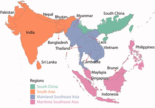
The Indo-Malaysian region, extending across most of South and Southeast Asia and into the southern parts of East Asia (Figure 1), is one of the eight biogeographic domains that is defined based on the distribution of terrestrial flora and fauna (Olson et al. 2001). It is home to nearly one third of the world’s population and some of the greatest biological diversity on the planet (Hughes 2018). The speed and scale at which human-induced environmental changes are taking place in the region make it a crucial focal point for assiduously documenting and analyzing land-cover and land-use changes (LCLUC; Stibig et al. 2007). Forest cover in Southeast Asia, for example, is disappearing at an alarming rate, with ∼63 percent (18,500 km²) of protected areas being deforested in West Kalimantan’s lowland from 1985 to 2001 (Curran et al. 2004). Coupled with the rapid urbanization of twenty-three megacities in South and Southeast Asia (Vadrevu et al. 2019), these changes invariably have pronounced effects on the climate system, sustainability, food and water security, biodiversity, and greenhouse gas emissions (Zeng et al. 2018). Yet despite the magnitude and importance of these LCLUCs to the Indo-Malaysian region, our knowledge concerning their patterns, rates, and transitions of land cover and land use (LCLU) remains limited, especially for South and Southeast Asia prior to 2000 (Achard et al. 2002). Estimates of tropical forest cover and its change still contain considerable uncertainties (Harris et al. 2012), as do existing satellite-derived trends in tropical deforestation rates from the 1990s to the 2000s (Stibig et al. 2014; Kim, Sexton, and Townshend 2015). In addition, previous work has tended to focus on forest–cropland transitions, thereby neglecting other important potential land transitions (Zeng et al. 2018). Together, these uncertainties undermine the assessment and development of land-use theory more generally (Allen and Barnes 1985; Walker and Solecki 2004; Turner et al. 2020) and policy in the region (Ivancic and Koh 2016; Hughes 2018) specifically. Moreover, these uncertainties generate ambiguities about the total carbon emissions from land-use change (Wang et al. 2020), and thus the global carbon budget (Achard et al. 2014).

Figure 1 Study area of the Indo-Malaysian region.

Considerable efforts have been made to establish accurate LCLU inventories in the Indo-Malaysian region. Inventory-based data, such as country-level annual forest area estimated by the United Nations Food and Agricultural Organization (FAO), based on country reports (FAO 2010), have been widely used. Yet, FAO data have been criticized for inconsistencies in the definition of forest among countries and over time, in part attributable to the challenge of standardizing national data obtained from different countries (Achard et al. 2002; Grainger 2008). In comparison, cropland area from the History Database of the Global Environment (HYDE), which relies on historical population statics (Goldewijk et al. 2017) provides a more internally consistent data set with a moderate spatial resolution of ∼0.083°. HYDE, however, is restricted temporally prior to 2000, when time steps coarsen to every ten years. These coverage gaps force spatial theoreticians and policy developers to rely on longer term LCLUC as a means to benchmark and advance their theories and policies, potentially missing more subtle drivers of LCLUC and policy levers to better manage such changes. Furthermore, as climate extremes manifest with regional heterogeneities (Intergovernmental Panel on Climate Change 2021), it is crucial to document and deconvolve the role of land-cover changes in altering such extremes, so that regional stakeholders are informed of how their land uses amplify the changing distribution of droughts, floods, and heat waves.

Remote sensing with repeated data coverage offers an indispensable way to enhance our capacity to monitor LCLUC (Roy et al. 2015). Some studies have demonstrated the scale of LCLUC in the portions of the Indo-Malaysian region using medium- to high-resolution data, such as that from repeated Landsat imagery (Abdullah et al. 2019). These studies are limited geographically, however (e.g., the coastal region of Bangladesh; Abdullah et al. 2019), or constrained to a short time period (e.g., 1985, 1995, and 2005; Roy et al. 2015), or focused on a particular land class (e.g., paddy rice; Xiao et al. 2006). As such, none of these studies can provide accurate LCLUC rates and explicit transitions, particularly dating back to the 1980s, nor can they depict interannual variability of these rates and transitions due to rapid rotations, such as logging of short-rotation forest (e.g., eucalyptus; Qiao et al. 2016). Such limitations generate uncertainty in the land-cover projections that currently are provided as boundary conditions in Earth system modeling efforts like the Coupled Model Intercomparison Project Phase 6 (CMIP6). What is clear is that for the Indo-Malaysian region, spatiotemporally completed LCLU maps with explicit vegetation types derived from long-term time-series remotely sensed data are of immense significance to robustly and exhaustively identify LCLUC patterns, rates, and transitions in the Indo-Malaysian region, and informing the downstream climate and carbon modeling efforts, as well as the land-use theory and policy communities.

There are some notable global LCLU products based on coarse-resolution data available, such as the Moderate-resolution Imaging Spectroradiometer (MODIS) land-cover data (MCD12Q1) from 2001 onward (Sulla-Menashe et al. 2019) and the European Space Agency (ESA) Climate Change Initiative (CCI) land cover maps from 1992 to 2018 (ESA 2017). Although these products provide a valuable source for LCLUC detection in the Indo-Malaysian region, they still cannot satisfy the need for temporal coverage prior to the 1990s. The latest released annual-scale Global Land Surface Satellite (GLASS) Global Land Cover (GLC) product covering from 1982 to 2015 fills some of this gap (H. Liu et al. 2020), but GLASS-GLC is trained at the global scale, ignoring the regional phenology of LCLU types, thereby creating additional classification uncertainty.

We address these shortcomings and generate an accurate assessment of the scale and speed of LCLUC in the Indo-Malaysian region. To do so, we apply a deep learning-based classification algorithm, namely temporal convolutional neural networks (TempCNNs) to produce an annual-scale, thirty-four-year LCLU inventory of maps for entire Indo-Malaysian region from 1982 to 2015 based on National Oceanic and Atmospheric Administration Advanced Very High Resolution Radiometer (AVHRR) Normalized Difference Vegetation Index (NDVI) data set. Because classification accuracy is sensitive to training samples, we explore classification skill of TempCNNs to different training data sources. To get robust accuracy information, this study not only validates our one-year (i.e., 2015) LCLU map based on an assumption of stationary map accuracy across years (the main validation procedure adopted by previous studies), but also uses 5,424 Landsat Thematic Mapper (TM) and Optical Land Imager (OLI) images from Google Earth Engine to validate the entire thirty-four-year series of classified LCLU maps. We do this to ensure our accuracy assessment of our classification is representative of the entire time series rather than just one year. Using this new data set, we ask and answer the following questions: (1) What are the spatiotemporal patterns of net and gross LCLUC in the Indo-Malaysian region over last three decades? (2) How have the rates of net LCLUC evolved over time? (3) What are the explicit transitions among different LCLU types?

Data

We use the second version of the AVHRR Global Inventory Modeling and Mapping Studies (GIMMS) NDVI third-generation data set (NDVI3g) from 1982 to 2015 to classify the land surface. The data set has a spatial resolution of 0.083° (approximately 8 km) and bimonthly temporal resolution (see https://ecocast.arc.nasa.gov/data/pub/gimms/3g.v1/). The GIMMS NDVI is generated from AVHRR/2 and three instruments and has been intercalibrated and corrected for atmosphere, cloud, and bias from the systematic orbital drift (Pinzon and Tucker 2014). Compared to its predecessors, NDVI3g extends its coverage to 2015 and shows more consistency in seasonal and interannual variability (Pinzon and Tucker 2014). The second version of NDVI3g has additional data quality information (i.e., flags of zero for a good value, one for a value estimated by spline interpolation, and two for a value estimated using a seasonal profile [given possible snow and cloud cover]). In this study, we only retain pixels with flag values of zero and one and exclude pixels with flag value of two, which leads to missing data in some regions and years (Figure S.1 in the Supplemental Material). Then we use a spatiotemporal gap filling method that relies on spatiotemporal subsets around the missing values (Gerber et al. 2018), named “gapfill,” to produce spatiotemporally complete NDVI values from 1982 to 2015 in the Indo-Malaysia region.

The MODIS Collection 6 land-cover data (MCD12Q1) are used as a reference source in this study (see https://earthdata.nasa.gov/). The MCD12Q1 provides global land-cover maps at an annual time step and 500-m spatial resolution from 2001 to 2018. The Collection 6 uses a hierarchical classification model with a random forest classifier based on MODIS reflectance data and has multiple classification schemes, including the seventeen-class International Geosphere-Biosphere Programme (IGBP; Sulla-Menashe et al. 2019). The accuracy of the IGBP-based version is ∼ 67 percent at the global scale. Compared to the Collection 5 product, spurious land-cover changes have been reduced by 9.8 percent (Sulla-Menashe et al. 2019). To ensure a consistent resolution with the AVHRR NDVI data, we resample the 500-m spatial resolution to 0.083° using a majority aggregation method following He, Lee, and Warner (2017). In this study, we use the IGBP seventeen-class legend, as it is one of the most commonly used land classification systems.

To test the performance of our classification algorithm to different reference data sources, we use another time series of LCLU from the ESA CCI (see http://maps.elie.ucl.ac.be/CCI/viewer/download.php), as an alternative to the Collection 6 training data. The CCI land-cover maps have a spatial resolution of 300 m, spanning from 1992 to 2018 at the annual scale (ESA 2017). The CCI land-cover data integrates reflectance data from multiple sensors, including Medium Resolution Imaging Spectrometer (MERIS), AVHRR, Project for On-Board Autonomy-Vegetation (PROBA-V), and so on (W. Li et al. 2018). The overall accuracy of this product is ∼71.5 percent validated against GlobCover 2009 (ESA 2011, 2017). The classification systems in the CCI land-cover data present two levels, a global legend with twenty-two classes, and a regional legend with thirty-seven classes (ESA 2017). Since the regional legend does not apply globally (ESA 2017), we use the global legend in this study. To be consistent with the MODIS IGBP legend, we translate the twenty-two CCI classes to the seventeen IGBP classes based on their class descriptions. We also use a majority aggregation method to resample the 300-m spatial resolution to 0.083°. We note that the CCI training data assimilates some AVHRR data, potentially undermining the exogeneity of our training and test data. This does not appear to be an issue here, however, for two reasons: First, CCI uses AVHRR surface reflectance (not NDVI, as we do) data. Second, we use the CCI from 2001 through 2013, which does not include the years in which the AVHRR reflectance data were assimilated, 1992 through 1999 (ESA 2017).

Methods

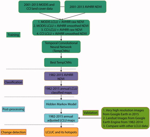
In this study, we use TempCNNs (Pelletier, Webb, and Petitjean 2019) as a classifier to generate our LCLU maps. The training data come from unchanged LCLU types from 2001 to 2013 derived from MODIS and CCI land-cover data, respectively. The accuracy is validated through visual interpretation of very high-resolution imagery from Google Earth in 2015 and 30-m resolution Landsat imagery from Google Earth Engine from 1982 to 2014. To evaluate the accuracy of our classified maps against other exiting LCLU data, we use the same validation data to assess the accuracy of MODIS, CCI, and GLASS-GLC LCLU maps in 2015. To remove some unreasonable LCLU transitions (e.g., urban–forest–urban in successive years), we apply a hidden Markov model (HMM) to smooth out these unrealistic transitions (Abercrombie and Friedl 2016). The procedure is summarized in Figure 2 and presented next.

Figure 2 Flowchart of methodology. Note: MODIS = Moderate-resolution Imaging Spectroradiometer; CCI = Climate Change Initiative; AVHRR = Advanced Very High Resolution Radiometer; NDVI = Normalized Difference Vegetation Index; LCLU = land cover and land use; LCLUC = land-cover and land-use change.

Classification and Postprocessing

Deep learning-based algorithms generally require a large amount of training data to learn model parameters and develop a skillful model (Abeßer 2020). We therefore use pixels of unchanged land cover from MODIS and CCI land-cover data for 2001 to 2013 as a reference data source (He, Lee, and Warner 2017). In doing so, we obtain more than 89,000 reference pixels for fourteen classes from MODIS data and some 100,000 pixels for fifteen classes from CCI data (Table S.1 in the Supplemental Material). Reconciling both performance skill and computational efficiency (Table S.2), the reference data are randomly split, with 67 percent used as training data and the remaining 33 percent used as testing data. We evaluate the influence of raw (i.e., unsmoothed) versus smoothed NDVI time series on the classification accuracy. Following He et al. (2015), we smooth the NDVI data using a double logistic method from TIMESAT, a widely used satellite time-series data processing software package (Jönsson and Eklundh 2004).

The classification is carried out using TempCNNs because of its flexibility in using temporal information. Deep learning approaches, such as recurrent neural networks (RNNs) and convolutional neural networks (CNNs), have been widely used in remote sensing classification (Zhong, Hu, and Zhou 2019). RNNs designed to analyze sequential data have a demonstrated potential for time series data classification (Sun, Di, and Fang 2019). RNNs are difficult to train, however, because of the large number of required layers and their distance from the classification output (Pelletier, Webb, and Petitjean 2019). Two- or three-dimension CNNs (2D/3D-CNNs) are commonly applied in spatial (i.e., x and y dimensions) and spectral (i.e., band) domains (Y. Li, Zhang, and Shen 2017), but rarely across the temporal dimension. As such, CNNs cannot take advantage of multitemporal information in time series data, like the AVHRR NDVI data we use in this study. TempCNNs estimated in one-dimension CNNs (1D CNNs) can be used across the temporal dimension. The pioneering works of Zhong, Hu, and Zhou (2019) and Pelletier, Webb, and Petitjean (2019) have proved the effectiveness and computational efficiency of the TempCNNs on time series classification at the local scale. The TempCNNs method outperforms traditional machine-learning algorithms like random forests as well as common RNNs, such as long-short term memory (Zhong, Hu, and Zhou 2019).

The TempCNNs—as in other deep learning networks—are based on the concatenation of different layers of automated learning, where each layer takes the outputs of the previous layer as inputs (Zhu et al. 2021). Each layer is composed of a certain number of units (i.e., neurons; Pelletier, Webb, and Petitjean 2019). TempCNNs have a user-selected number of hidden layers of weights, as well as other hyperparameters that must be optimized based on the trade-off between accuracy and computational intensity (Zhu et al. 2021). Based on Pelletier, Webb, and Petitjean (2019) and our experiments, we use three convolutional layers (each with sixty-four neurons), one dense layer (256 neurons), and one Softmax layer with Adam optimization (default parameter values: β₁ = 0.9, β₂ = 0.999, ε = 10⁻⁸). We choose a training sample size (i.e., batch size) of sixty-four, which means sixty-four samples from training data to train the network in each training iteration, and a maximum number of epochs set to forty to completely pass the entire training data set forty times through the network (Zhu et al. 2021). In this study, we apply the TempCNNs in the temporal domain (i.e., twenty-four NDVI values per year) without considering spatial structure. The algorithms are built using the Keras library (https://keras.io/) on top of Tensorflow (https://www.tensorflow.org/).

To further assess the performance of TempCNNs, we also compare it with the widely used random forest classifier. The random forest classifier is made up of a large number of classification trees, which vote to produce a single outcome for each pixel (Breiman 2001). It requires two user-defined parameters: the number of decision trees produced (ntree) and the number of variables available for splitting at each node (mtry). We chose a value of 500 for ntree and the default value (i.e., the square root of the number of predictor variables) for mtry based on He, Lee, and Warner (2017). To train the random forest classifier, we extract nineteen phenological metrics from the smoothed 1982 through 2015 NDVI time series, such as the start of growing season, the end of growing season, and the maximum NDVI values (Table S.3 in the Supplemental Material). We use phenological information as it can improve the classification accuracy of a random forest approach (Zhong, Hu, and Zhou 2019). The random forest classification is implemented in R using the “randomForest” package.

Because there is the possibility for classification errors to result in unreasonable high-frequency land-cover transitions (e.g., forest to urban and then back to forest in successive years), we apply the HMM to smooth out these unrealistic transitions (Abercrombie and Friedl 2016). HMMs describe a series of unknown states that can be inferred from a sequence of observations (Rabiner 1989). In the context of annual land-cover mapping, the unknown states are the land-cover labels assigned to each pixel, and the observations are remote sensing measurements (i.e., NDVI in this study). HMMs have been used to successfully generate spatial-temporal consistent land-cover maps (Gong et al. 2017).

Accuracy Assessment

We use the traditional validation method of a confusion matrix to assess the accuracy of our classified LCLU maps (Olofsson et al. 2014). In general, remote sensing validation assumes stationarity of accuracy across years and only validates maps of the most recent years due to the scarcity of reference data in earlier years (Gómez, White, and Wulder 2016). In this study, we build a validation data set using visual interpretation of recent (2015) very high-resolution satellite images in Google Earth. Based on the stratified sampling scheme, we randomly select 350 sample points with a minimum of sixteen points for each mapped class (i.e., each class is a stratum) in this study across the study area with a desired precision of 10 percent and significance level of 0.15. Our selection of 350 points represents more than a doubling of the suggested number of validation points needed based on Jensen’s (2016) equation. We then generate a 0.083° × 0.083° square centered on these sample points, representing the AVHRR pixel domain. To validate the 2015 classified map, we examine these grid squares in Google Earth and visually interpret the very high-resolution imagery available within those pixels. We then assign a majority class to each pixel based on our assessment from the high-resolution imagery. Two independent analysts separately perform this visual interpretation on the same data, providing a quantitative metric of the robustness and uncertainty of this visual validation interpretation process. Sample points without appropriate very high-resolution images in 2015 are removed, leaving a final total of 309 sample points. We combine evergreen needleleaf forest, evergreen broadleaf forest, deciduous broadleaf forest, and mixed forest into a single forest class, and savannas and woody savannas into a single savanna class, as it is not always possible to differentiate them. Although the original map has fourteen classes (Table S.1), the accuracy assessment is based on ten of those classes.

In an effort to provide the most reliable accuracy information, we also build a spatiotemporal validation data set using visual interpretation of 5,424 historical (1982–2014) Landsat TM and OLI satellite images, accessed via Google Earth Engine (Figure S.2 in the Supplemental Material). In doing so, we assess the accuracy for the most recent year as traditionally done, as well as for the entire time period of classification. We extract cloud-free median Landsat image composites (including Landsat 4, 5, and 8) for each 0.083° × 0.083° square during the growing season (i.e., May–October) for each year from 1982 to 2014. We also extract Landsat imagery for the dry season (i.e., December–February and March–May) to maximize the availability of validation data. We choose the median composite, rather than the mean composite, as the median is less affected by outliers. By comparing different color composites (i.e., true and false color composites), we are able to visually interpret and assign the dominant class to each sample image.

Based on these sample points with known classes and our classified LCLU maps, we follow Olofsson et al. (2014) and Pontius and Millones (2011) to generate a population confusion matrix by estimating the cell entries using Equation 1(1) $$P_{ij}=W_i\frac{n_{ij}}{n_{i+}}$$(1) . (1) $$P_{ij}=W_i\frac{n_{ij}}{n_{i+}}$$(1) where $P_{ij}$ is the proportion of area for the population that is class i according to the classified map and class j according to the reference map. $W_i$ is the proportion of area mapped as class i. $n_{ij}$ is the number of samples in class i according to the classified map and class j according to the reference map. $n_{i+}$ denotes the row sums.

We then calculate the corresponding producer’s, user’s, and overall accuracy and assess the uncertainty in each of these accuracy assessments via a bootstrapping methodology. We also follow Pontius and Millones (2011) to calculate allocation disagreement and quantity disagreement, thereby partitioning the total error into components related to errors in class location and proportion. To evaluate the accuracy of our classified maps with other existing LCLU data, we use the same sampling data to assess the accuracy of MODIS, CCI, and GLASS-GLC LCLU maps in 2015.

LCLU Change Detection

To reveal spatial patterns of LCLUC, we first regrid our classified data to a 0.5° scale and calculate percentage of gross changes (i.e., gross gain and gross loss) between consecutive years for each LCLU type in each grid cell. The net changes between consecutive years are determined by adding gross gains to gross losses. We then calculate the cumulative thirty-four-year gross and net changes to demonstrate how LCLU changes have varied spatially over the last three decades.

To explore temporal patterns of LCLUC, we calculate areas for each LCLU type over four subregions in the Indo-Malaysian region (i.e., South China, South Asia, mainland Southeast Asia, and maritime Southeast Asia) and conduct linear regression trend analysis (following the methods of He et al. [2018]) for each class in each region. For the main LCLU types (e.g., forests), we also calculate each country’s contribution to the areas of each LCLU type in the corresponding subregion (e.g., areas of forests in India/total areas of forests in South Asia). We then calculate the cumulative change of these thirty-four-year time series to demonstrate LCLUC rates and how these rates change over time for each region as follows. (2) $$\Delta {\mathit{change}\mathrm{ }of\mathrm{ }\mathit{LCLU}}_{i,t}={\mathit{Area}\mathrm{ }of\mathrm{ }\mathit{LCLU}}_{i,t}-{\mathit{Area}\mathrm{ }of\mathrm{ }\mathit{LCLU}}_{i,t-1}$$(2) (3) $$\mathrm{Cumulative}\mathrm{ }{\mathit{change}\mathrm{ }of\mathrm{ }\mathit{LCLU}}_{i,t}=\mathrm{ }\sum _{1983}^t\Delta {\mathit{change}\mathrm{ }of\mathrm{ }\mathit{LCLU}}_{i,t}$$(3) where i represents each LCLU type (e.g., forests) and t is the year from 1983 to 2015.

We further examine the explicit land-class transitions that take place in each 0.083° grid cell in the Indo-Malaysian region. We focus on dominant loss transition of each LCLU type to other types over the last thirty-four years. The dominant loss transition is determined by the most frequent transition over the study period. For instance, if the transition of forests to shrublands occurred most times, the corresponding grid cell is assigned to the transition of forests loss to shrublands. To reveal how much LCLU experienced changes, we also calculate the percentage of each LCLU type experiencing dominant loss transitions over the four subregions, respectively, using Equation 4(4) $${\mathit{Percentage}\mathrm{ }of\mathrm{ }\mathit{changed}\mathrm{ }\mathit{LCLU}}_{i,j}=\frac{{\mathit{Area}\mathrm{ }of\mathrm{ }\mathit{LCLU}}_{i,j}\mathrm{ }\mathit{experiencing}\text{ dominant loss }\mathit{transitions}}{{\mathit{Area}\mathrm{ }of\mathrm{ }\mathit{total}\mathrm{ }\mathit{LCLU}}_{i,j}}\times 100\mathrm{\%}$$(4) . (4) $${\mathit{Percentage}\mathrm{ }of\mathrm{ }\mathit{changed}\mathrm{ }\mathit{LCLU}}_{i,j}=\frac{{\mathit{Area}\mathrm{ }of\mathrm{ }\mathit{LCLU}}_{i,j}\mathrm{ }\mathit{experiencing}\text{ dominant loss }\mathit{transitions}}{{\mathit{Area}\mathrm{ }of\mathrm{ }\mathit{total}\mathrm{ }\mathit{LCLU}}_{i,j}}\times 100\mathrm{\%}$$(4) where i represents each LCLU type (e.g., forests), and j denotes each region in the Indo-Malaysian region. Please note, if a pixel experiences several times of dominant loss transition, the pixel is still counted only once to avoid undue weight to nonpermanent changes. The total area of certain LCLU type counts all pixels that emerge as this LCLU type over the thirty-four years. We also calculate the percentage of each LCLU type experiencing dominant gain transitions following the same method.

Results

TempCNNs Performance Skill

The overall accuracy of TempCNNs varies across different combinations of training sources and NDVI smoothing (Table 1). With an overall accuracy of 81.50 percent, the TempCNNs perform best when we use raw NDVI and MODIS land-cover data as reference data. It has somewhat reduced accuracy when the NDVI data are smoothed by a double-logistic function (76.89 percent) or when raw NDVI is combined with the CCI data (76.80 percent). Performance accuracy is further reduced when the CCI data combined with the smoothed NDVI (72.03 percent). As such, the TempCNNs using MODIS data outperform that with CCI data, which one could suggest is due to our aggregation of CCI classes to match those from MODIS. Even with original CCI classes, however, the TempCNNs still have poorer accuracy compared to that with MODIS data (Table S.4 in the Supplemental Material), indicating our aggregation of the CCI data is not a cause for the reduced performance of CCI relative to MODIS. The TempCNNs using raw NDVI and MODIS reference sources also outperform the random forest classifier based on the smoothed NDVI time series (78.2 percent).

Table 1. Performance skill of temporal convolutional neural networks (TempCNNs) for different reference sources and Normalized Difference Vegetation Index (NDVI) smoothing

Reference source	NDVI status
	Raw NDVI	Double-logistic smoothed NDVI
MODIS	81.50%	76.89%
CCI (IGBP class)	76.80%	72.03%

Note: MODIS = Moderate-resolution Imaging Spectroradiometer; CCI = Climate Change Initiative; IGBP = International Geosphere-Biosphere Programme.

Accuracy Assessment of Classified Maps

Classification Validation. We use the raw NDVI and MODIS land-cover data as reference data to train the TempCNNs classifier and subsequently generate a thirty-four-year time series of annual LCLU maps for the Indo-Malaysian region. Our 2015 classified map validated using very high-resolution imagery has an overall accuracy of ∼81 percent (Figure 3). The consistency of visual interpretations between independent analysts working with the same set of validation sites is 90.1 percent. We also select 90 percent of the very high-resolution imagery and use a bootstrapping method to repeat the process 1,000 times. The accuracy is coherent (Table S.6 in the Supplemental Material). Forests, savannas, croplands, and barren show a relatively high producer’s and user’s accuracy (>69 percent), whereas open shrublands have low accuracy scores (<29 percent; Figure 3). Grasslands and permanent wetlands have high producer’s accuracy (100 percent) but low user’s accuracy (25 percent and 13 percent, respectively), indicating that even though 100 percent of the reference grasslands and permanent wetlands have been correctly identified in the map, only 25 percent and 13 percent of the two types identified as grasslands and permanent wetlands in the classified map are actually grasslands and permanent wetlands. This is due to misclassification of croplands to grasslands and permanent wetlands (Table S.5 in the Supplemental Material). The user’s accuracy for urban and built-up land and water bodies is relatively high (>77 percent), but the producer’s accuracy is low (<29 percent), denoting that only <29 percent of the reference sites for these two classes have been correctly identified in the classified map, with croplands being the most common incorrectly assigned class for both of them (Table S.5).

Figure 3 Validation of classified land cover and land use (LCLU) maps for 2015 using the very high-resolution reference data (the sum of overall accuracy, allocation, and quantity disagreements equals 100 percent).

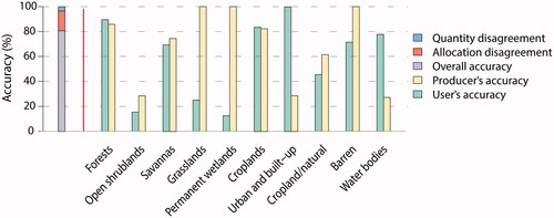
We further assess the allocation and quantity disagreements for the classification. Quantity disagreement is a summary measure of the difference between the reference and classified maps in the proportions of the classes, and allocation disagreement summarizes the difference between the reference and classified maps in the spatial allocation of the categories (Pontius and Millones 2011). The allocation and quantity disagreements are 16 percent and 3 percent, respectively (Figure 3). This indicates that the classification error is mainly because of a spatial location mismatch for classes between the reference map and our classified map.

Using the historical Landsat image archive, we validate the remainder of the time series, finding the overall accuracy as ∼84 percent, with an allocation disagreement of 13 percent and a quantity disagreement of 4 percent for the eight classes available for evaluation (Figure S.3 in the Supplemental Material), which is only 3 percent higher than the 2015 validation with ten classes (Figure 3). Except for permanent wetlands, the producer’s and user’s accuracy are similar to those found in our 2015 validation. This implies that our classification error is stationary across years and supports the general practice in remote sensing validation of using a single year to evaluate the accuracy of a multiyear classification when a consistent methodology is used in all years.

Intercomparison with MODIS, CCI, and GLASS-GLC Land Cover Data. To further evaluate the accuracy of our classified maps, we compare our classification to other LCLU products from MODIS, CCI, and GLASS-GLC. Because those LCLU data have different classes (i.e., fourteen classes for our classified maps and MODIS, twenty-two for CCI, and seven for GLASS-GLC), we convert them into a common five-class system based on their respective class descriptions (i.e., forests, shrublands, grasslands, croplands, and barren).

We validate these five-class maps for 2015 using our very high-resolution imagery reference data set, finding our original classified map to have an overall accuracy of 88 percent, higher than that from classifications produced by MODIS (84 percent), GLASS-GLC (81 percent), and CCI (79 percent) LCLU data (Figure S.4 in the Supplemental Material). Except for CCI LCLU data, the allocation disagreement is higher than quantity disagreement, indicating that location mismatches for classes between the reference map and our classified map are the dominant source for classification error. Forests and croplands have a relatively high producer’s and user’s accuracy (> 76 percent) for all of four LCLU data, whereas shrublands have the poorest accuracy (Figure S.4). Nevertheless, the intercomparison we provide across other classifications supports the reliability of our classified maps.

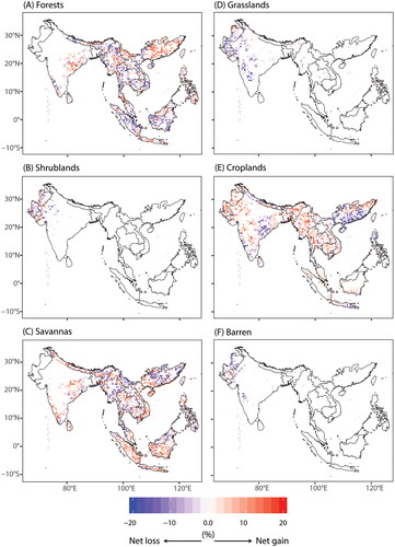
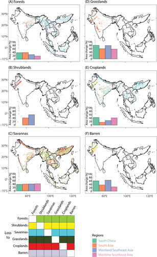
Figure 4 Spatial distributions of cumulative net changes of land cover and land use (LCLU) types from 1982 to 2015 presented as the percent change in that class in each half-degree grid cell. (A) Forests, (B) shrublands, (C) savannas, (D) grasslands, (E) croplands, and (F) barren lands.

Rapid LCLUC in the Indo-Malaysian Region

Spatial Patterns of LCLUC. Building on our thirty-four-year classified LCLU data, we conduct several spatiotemporal analyses to detect LCLU changes. Our results show that Indo-Malaysia experienced extensive gross and net LCLUC during the last three decades, with forests, shrublands, grasslands, savannas, croplands, and barren showing the most dramatic changes (Figure 4; Figure S.5 in the Supplemental Material). Forests have increased their coverage in South China and parts of South Asia, including eastern coastal regions in India, and decreased in most regions of mainland and maritime Southeast Asia, including Thailand, Cambodia, Laos, Vietnam, Malaysia, and Indonesia (Figure 4A). In contrast to the increasing forest coverage in those regions, croplands have decreased in South China and the eastern part of India; at the same time, crops have increased across mainland and maritime Southeast Asia, the western part of India, and throughout Pakistan (Figure 4E).

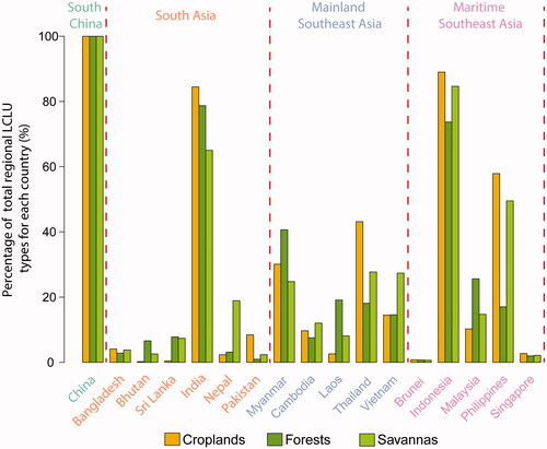
Figure 5 Mean percentage of forests, croplands, and savannas for each country relative to their regional totals averaged from 1982 to 2015. Regions are separated by dotted red lines. Note: LCLU = land cover and land use.

Notably, savannas have decreased in South China, and some parts of mainland Southeast Asia, such as Myanmar (Figure 4C), a change overlooked by previous studies. These savannas are either restored to forests or have been converted to croplands. Shrublands, grasslands, and barren lands experienced relatively small changes over the period of analysis, with modest shrublands decreasing in Pakistan (Figure 4B), grasslands decreasing in Pakistan and western India (Figure 4D), and barren lands decreasing in Pakistan (Figure 4F).

These spatial change patterns for each land-cover type are reinforced by the results of a test involving upscaling our classified LCLU data to 1° (Figure S.6 in the Supplemental Material). For instance, the decrease of forests in mainland and maritime Southeast Asia and increase in croplands in these two regions are also identified in the 1° data (Figure S.6). This suggests that our regridding choice does not introduce uncertainty in the change patterns we identify.

Figure 6 Area of land cover and land use (LCLU) types and their temporal changes from 1982 to 2015. The solid lines represent cumulative area change for each LCLU type in each region following Equations 2(2) $$\Delta {\mathit{change}\mathrm{ }of\mathrm{ }\mathit{LCLU}}_{i,t}={\mathit{Area}\mathrm{ }of\mathrm{ }\mathit{LCLU}}_{i,t}-{\mathit{Area}\mathrm{ }of\mathrm{ }\mathit{LCLU}}_{i,t-1}$$(2) and 3(3) $$\mathrm{Cumulative}\mathrm{ }{\mathit{change}\mathrm{ }of\mathrm{ }\mathit{LCLU}}_{i,t}=\mathrm{ }\sum _{1983}^t\Delta {\mathit{change}\mathrm{ }of\mathrm{ }\mathit{LCLU}}_{i,t}$$(3) . The numbers represent the area trend (km² per year). *, **, and *** denote 10 percent, 5 percent, and 1 percent significance levels, respectively. (A) Forests, (B) shrublands, (C) savannas, (D) grasslands, (E) croplands, and (F) barren lands.

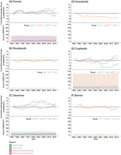
Temporal Patterns of LCLUC. Forests, croplands, and savannas dominate the Indo-Malaysian landscape (Table 2), with China, India, Myanmar, Thailand, Indonesia, and the Philippines having the highest proportions of those classes (Figure 5). Forests in mainland Southeast Asia decreased from ∼768,192 km² in 1982 to ∼727,552 km² in 2015, indicating a loss of ∼5.29 percent (Figure 6A). The linear trend indicates forests significantly decreased by ∼1,297 (±411) km² per year (Figure 6A), accounting for ∼0.17 percent forest loss per year in this region. Similarly, the forest cover in maritime Southeast Asia decreased by ∼7.18 percent to ∼805,760 km² in 2015, with an overall decreasing trend of ∼664 (±358) km² per year (∼0.07 percent per year; Figure 6A), whereas South Asia experienced a slight forest gain, with an overall increasing trend of 787 (±312) km² per year (∼0.32 percent per year; Figure 6A). Forests in South China increased massively by ∼63.49 percent to ∼240,448 km² (Figure 6A), indicative of widespread landscape changes. The overall increasing rate of forest cover in South China is ∼2,211 (±420) km² per year, equivalent to ∼1.29 percent forest gain per year (Figure 6A). In fact, croplands decreased in South China by nearly the half amount of forest gain, from ∼215,488 km² in 1982 to ∼153,792 km² in 2015, a net decrease of ∼28.63 percent (Figure 6E). The significant rate of cropland loss in South China is 3,767 (±469) km² per year (∼2.36 percent per year; Figure 6E). In contrast, croplands in mainland Southeast Asia increased by ∼9.10 percent to ∼420,608 km² in 2015, with an overall significant rate of increase of 763 (±262) km² per year (∼0.19 percent per year; Figure 6E). South Asia and maritime Southeast Asia had essentially no significant change in croplands (Figure 6E), which is likely due to the contrast spatial patterns of croplands within the regions (Figure 4). Unlike forests and croplands, Savannas have consistent increasing patterns over all the four regions (Figure 6C). Savannas in South Asia, mainland, and maritime Southeast Asia increased by 21.46 percent, 1.14 percent, and 48.15 percent to totals of 288,320 km², 328,448 km², and 179,584 km² in 2015, respectively (Figure 6C). Savannas in South China decreased from 488,064 km² in 1982 to 455,488 km² in 2015. The overall increase trend, however, is some 1,477 (±546) km² per year (∼0.28 percent per year), largely driven by their expansion in the 2000s (Figure 6C).

Table 2.  Mean proportion of each land cover type in each region averaged from 1982 to 2015

LCLU type	Region
	South China	South Asia	Mainland Southeast Asia	Maritime Southeast Asia
Barren	0.010%	5.859%	0.023%	0.001%
Cropland/natural vegetation mosaics	0.107%	0.156%	0.647%	5.378%
Croplands	18.567%	70.696%	26.133%	2.397%
Forests	19.654%	7.984%	52.002%	81.300%
Grasslands	0.191%	2.192%	0.076%	0.003%
Permanent wetlands	0.002%	0.066%	0.002%	0.002%
Savannas	60.734%	9.420%	20.751%	10.199%
Shrublands	0.000%	3.178%	0.002%	0.000%
Urban and built-up	0.442%	0.144%	0.110%	0.131%
Water bodies	0.293%	0.304%	0.254%	0.589%

Note: LCLU = land cover and land use.

Although grasslands and barren lands occupy relatively small areas in the Indo-Malaysian region, they experienced large changes over the period evaluated. Grasslands decreased by approximately 77 percent, 68 percent, and 74 percent to ∼512 km², 38,272km², and 640 km² by 2015 in South China, South Asia, and mainland Southeast Asia (Figure 6D), respectively, with an overall decreasing trend of ∼67 (±18) km² per year, ∼2,037 (±199) km² per year, and ∼38 (±8) km² per year (∼4.15 percent per year, 3.07 percent per year, and 3.35 percent per year), respectively. Barren lands decreased by some 13.14 percent and 80 percent to ∼159,936 km² and 128 km² by 2015 in South Asia and mainland Southeast Asia (Figure 6F), with an overall decreasing trend of ∼1,193 (±348) km² per year and ∼15 (±1) km² per year (∼ 0.67 percent per year and 4.50 percent per year).

Unlike the assessments of regional LCLUC in previous studies (e.g., DeFries et al. 2002), the change patterns we identify are not monotonic over the last three decades: Some years exhibit increasing trends, whereas others have decreasing trends (Figure 6). Documenting the interannual variation in LCLU changes, as we have done here, positions a much richer analysis of the drivers and variation in LCLUC, as well as the evaluation of the success or failure of different land management policies in different regions. In mainland Southeast Asia, for example, forests decreased in 1983 and 1989, whereas they increased in other years during the 1980s, leading to a cumulative increase of ∼48,768 km² (∼6.28 percent) over the 1980s (Figure 6A), whereas forests decreased during the early and later 1990s. Together these variations resulted in a cumulative forest loss of ∼49,920 km² (∼6.43 percent) over the 1990s. This forest loss reversed in the 2000s, leading a net gain of 320 km² (∼0.04 percent). In the 2010s, forests then had a net loss of ∼39,808 km² (∼5.13 percent). These fluctuations of forest cover induced a cumulative decrease in forested area of 40,640 km² (∼5.23 percent) in mainland Southeast Asia over the last thirty-four years (Figure 6A). In maritime Southeast Asia and South Asia, forests show similar fluctuations. Forest cover in maritime Southeast Asia increased in most years during the 1980s with a cumulative increase of ∼45,248 km² (5.08 percent; Figure 6A), followed by a cumulative decrease in forests of ∼21,504 km² (2.41 percent) in the 1990s. It then returned to a cumulative increase of ∼12,736 km² (1.43 percent) in the 2000s, followed by a cumulative decrease of ∼98,816 km² (11.09 percent) in the 2010s, leading to an overall net loss of forests of 62,336 km² (7.00 percent) in maritime Southeast Asia during last three decades (Figure 6A). Forests in South Asia showed a cumulative increase in the 1980s of ∼53,248 km² (∼21.86 percent) and of ∼30,400 km² (∼12.48 percent) in the 2000s. The large loss of forests in 1990, 1991, and 1999 led to a cumulative loss of ∼36,800 km² (∼15.11 percent) in the 1990s. Forests also decreased in the 2010s with a cumulative loss of 45,056 km² (∼18.50 percent). The cumulative change of forests in South Asia over the last thirty-four years represented a net decrease of 1,792 km² (∼0.7 percent). In South China, forest cover increased during the 1980s, 2000s, and 2010s with a cumulative increase of ∼28,352 km², ∼80,640 km², and ∼13,696 km² (∼16.56 percent, 47.11 percent, and 8.00 percent), respectively, although some years show large decreasing rates (e.g., 2000 and 2011). The relatively large loss of forests in 1991, 1992, and 1999 led to a cumulative loss of some 29,312 km² (∼17.12 percent) of Southern Chinese forests during the 1990s. Yet the cumulative increase of forests (93,376 km² [∼54.55 percent]) in South China over the full period we consider (Figure 6A) indicates the effectiveness of afforestation projects.

Croplands in South China experienced a large decrease in 1985, contributing to a cumulative loss of some 18,176 km² (∼11.39 percent) in the 1980s (Figure 6E). The decrease continued through the 1990s and 2000s, netting a loss of 14,080 km (∼8.83 percent), and 93,440 km² (∼58.57 percent) in those decades, respectively. Yet crops expanded massively in the 2010s, increasing by ∼64,000 km² (∼40.12 percent). Despite these recent crop expansions, over the three-decade period, the net effect has been a cropland decrease of 61,696 km² (∼38.67 percent; Figure 6E). In South Asia, the large increase of croplands in 1983 and 1988 led to a modest cumulative gain of ∼9,344 km² (∼0.43 percent) during the 1980s, although croplands decreased in other years in this decade (Figure 6E). It is followed by a cumulative decrease of 22,912 km² (∼1.06 percent) in the 1990s, and 2,176 km² (∼0.10 percent) in the 2000s with some years experiencing large increases (e.g., 1991, 1994, 1999, and 2007), followed by a massive expansion in the 2010s with a cumulative increase of 100,224 km² (∼4.63 percent), resulting in an overall cumulative increase of 84,480 km² (∼3.90 percent) during the last thirty-four years for the South Asian region (Figure 6E). In mainland Southeast Asia, croplands expanded by ∼478 percent between the 1980s and the 2010s, with a net gain of 23,680 km² (∼6.04 percent). This acceleration is punctuated, however, by a rapid ten-year decrease in croplands in the 1990s with a cumulative loss of some 19,904 km² (∼5.08 percent), inducing an overall cumulative gain for the region of 35,072 km² (∼8.95 percent; Figure 6E). Such variations position finer scale investigations of country-level policies or market forces that can account for such dramatic decade-to-decade changes. Furthermore, these changes suggest that there is a large-scale conversion among land-cover types, such as a conversion of forests to croplands or vice versa, leading to the next step in our analysis evaluating land-cover transitions.

LCLU Transitions. Most previous research on LCLUC across these regions has focused on the transitions between forests and croplands (Xu, Jain, and Calvin 2019). In contrast, our study further explores comprehensive transitions among all classified LCLU types (Figure 7 and Figure S.8 in the Supplemental Material). Our results demonstrate forests principally become savannas (likely newly cleared forests) or croplands with ∼38.02 percent, 38.80 percent, 26.98 percent, and 18.54 percent of forests in South China, South Asia, and mainland and maritime Southeast Asia experiencing these transitions over the 1982 to 2015 period (Figure 7A). Areas classified as savanna tend to transition to forests or croplands in South China, mainland Southeast Asia, and parts of South Asia. More than 38 percent of savannas in the Indo-Malaysian region experienced such transitions (Figure 7C), indicating extensive changes in savannas coverage, with likely implications for net changes in above-ground carbon in the region. The transition of grasslands to croplands is primarily centered on South Asia, with ∼59.79 percent of grasslands in this region undergoing changes (Figure 7D). Some 44.00 percent, 15.97 percent, 26.68 percent, and 41.63 percent of croplands in South China, South Asia, and mainland and maritime Southeast Asia, respectively, experience transitions to savannas, forests, or shrublands (Figure 7E). Some 41.43 percent and 36.19 percent of shrublands and barren lands in South Asia undergo dominant transitions (Figure 7B and 7F). Together with Figure 4, we can infer that net decreasing forest cover in maritime Southeast Asia is presumably due to the increase of savannas (Figure 4A and 4C, Figure 7A). In contrast, the expansion of forests in South China is predominantly because of decreasing savannas (Figure 4A and 4C, Figure S.8A). The expansion of croplands in mainland Southeast Asia comes to the sacrifice of forest and savanna lands (Figure 4A, 4C, and 4E, and Figure S.8E), whereas the increasing of croplands in western part of India is mainly due to loss of grasslands (Figure 4D and 4E, Figure 7D).

Figure 7 Transitions of (A) forests, (B) shrublands, (C) savannas, (D) grasslands, (E) croplands, and (F) barren lands that are lost to other land cover and land use (LCLU) types. The inset bar plot in each panel represents the percentage of each LCLU type experiencing dominant loss transitions over each region (see legend) following Equation 4(4) $${\mathit{Percentage}\mathrm{ }of\mathrm{ }\mathit{changed}\mathrm{ }\mathit{LCLU}}_{i,j}=\frac{{\mathit{Area}\mathrm{ }of\mathrm{ }\mathit{LCLU}}_{i,j}\mathrm{ }\mathit{experiencing}\text{ dominant loss }\mathit{transitions}}{{\mathit{Area}\mathrm{ }of\mathrm{ }\mathit{total}\mathrm{ }\mathit{LCLU}}_{i,j}}\times 100\mathrm{\%}$$(4) .

Discussion

A possible reason for the better performance of TempCNNs using MODIS data compared to that with CCI data is that multiple satellite sources are used to produce CCI land-cover data, which leads to inconsistent accuracy of CCI data across years (ESA 2017). This could bring additional uncertainty when we generate reference classes, and thus influence the overall classification accuracy. The performance of TempCNNs with raw NDVI is superior to that with smoothed NDVI (Table 1) and random forest classifier with phenological metrics, presumably due to the fact that the double-logistic function smooths out the rapid changes in land-cover classes, like crops, or overfits stationary classes, like long-lived evergreen broadleaf forests (Zhong, Hu, and Zhou 2019).

Validated against very high-resolution images in Google Earth and Landsat images, we find poor performance of the TempCNNs over open shrublands, which is also identified in Ayhan and Kwan (2020). This is likely attributable to the relatively small training sample size for that class (Table S.1). It could be also caused by the misclassification of shrublands and croplands (Table S.5) in dryland areas, as the two classes share a similar NDVI signature in drylands. The misclassifications of croplands with urban and built-up land, grasslands, permanent wetlands, and water bodies arise from several possibilities. The coarse resolution of the input data and the places in which crops are grown (e.g., crops cultivated near urban areas) results in mixed-class pixels. Complicating the algorithm’s separation of crops versus grasslands is the similar phenology of the two, whereas those croplands inundated with water from irrigation or monsoons would lead to their misclassifications as water bodies. We find that the classification error is mainly attributable to a spatial location mismatch for classes between the reference map and our classified map, an issue also identified in previous studies (e.g., Ruelland et al. 2008). The misclassification of croplands, forests, open shrublands, and savannas due to similar annual cycles of NDVI (e.g., similar maximum NDVI for oil palm crop, forests, and savannas), natural climate influences (e.g., dry year leads to the abandonment of croplands), and missing NDVI values (Figure S.1) largely contribute to the disagreements (Table S.5). Improving the classification feature selections of these classes and NDVI filling algorithms can reduce the disagreements, enhancing the overall accuracy.

Based on our classified maps, we identify the rapid LCLUC in the Indo-Malaysian region spatially and temporally. The net decreasing pattern of forests in Southeast Asia identified in this study has been documented in previous studies (Achard et al. 2002; Stibig et al. 2014; W. Li et al. 2018), although the study periods in those efforts are considerably shorter than ours, emphasizing that such deforestation is a long-term trend, underpinned by years of rapid conversion and years of slower change. There are several underlying causes of decreasing forests in Southeast Asia, including shifting cultivation, illegal logging, forest fires, and the expansion of agricultural lands (Giri, Defourny, and Shrestha 2003). The net increase of forests in India and South China is consistent with the findings of He, Lee, and Warner (2017) and Vadrevu et al. (2019), which those studies attribute to sustainable afforestation measures, such as the Grain for Green project in China (J. Liu et al. 2014) and the Green India Mission in India (Seidler and Bawa 2016). Consistent with previous results (J. Liu et al. 2014; He et al. 2018), the decreasing croplands in South China could be due to afforestation projects. The expansion of croplands in South and Southeast Asia is not only because of intense population pressure, but also due to natural drivers, which can lead to crop abandonment in some dry years (Xu, Jain, and Calvin 2019).

The forest expansion we identify during the 2000s in Southeast Asia contradicts the results reported by Stibig et al. (2014), which documented a decrease. The incongruence is likely attributable to the different temporal resolution of the data: our annual data versus their decadal data. The discrepancy could also be due to the coarse 8-km spatial resolution of our NDVI data, however, which could lead to misclassifications, mistaking commodity crops (e.g., oil palm plantation) as forests. At the same time, however, the deceleration of deforestation from the 1990s to 2000s we identify is consistent with the findings from FAO (2010). Our findings also complicate the results from Kim, Sexton, and Townshend (2015) that documented an acceleration of humid tropical forest loss. Such a discrepancy is partly attributable to the inconsistent land cover definitions of the forest class in our study versus that of Kim, Sexton, and Townshend (2015). On croplands, our findings tend to confirm earlier ones. For example, the decreased rate of cropland change in the 1990s to 2000s in South China is consistent with findings from J. Liu et al. (2005) and Gao et al. (2019). At the same time, however, we document a larger magnitude of cropland rate change than those studies, presumably because we consider a different domain. Moreover, the coarse resolution of our data might overestimate cropland areas. The year-to-year variation in the rate of change in forested and cropland areas could partly arise from classification errors. It might also be possible, for example, as one place experiences increasing forests, other places could experience decreasing forests (Figure S.7 in the Supplemental Materials). Nevertheless, we expect these errors to be stochastic, rather than trending in time or space. Randomly distributed classification errors lend confidence to our interpretation that the net changes of LCLU types we document imply complex interactions among policy and land management. Together, our results emphasize the importance of real-time monitoring, or at the very least, change detection assessments over shorter intervals.

The transition of forests to croplands in mainland Southeast Asia confirms previous work (Zeng et al. 2018) and is consistent with theory about economic drivers of land-use change. The transitions of savannas to forests in South China was previously attributed to conversion of grasslands or croplands (J. Liu et al. 2014), although savannas might have been previously converted from croplands (Figure 7), indicating savannas could be a bridge from croplands to forests in South China. The transitions between forests and savannas we demonstrate here also indicate the potential restoration or degradation of forests or logging and regrowth of short-rotation forests, which, with further country-scale analysis, could provide important insights for future land management practices. The large extent of changes happening in minor LCLU types (i.e., grasslands and barren lands) imply an overlooked importance of secondary LCLU types and suggest that those land cover types require more attention by both the theoretical and policy communities in the region.

Conclusion

We have documented the rapid LCLUC in the Indo-Malaysian region since 1982, the rates, patterns, and magnitudes of which were not fully documented or understood, particularly given their scale and speed. A spatially complete and temporally continuous LCLU data set of Indo-Malaysia is crucial for understanding its LCLU drivers and environmental consequences, as well as implementing future conservation measures, land theory development, or assessing regional-scale contributions to carbon emissions.

Here we rigorously evaluate the use of TempCNNs to document nearly thirty-five years (1982–2015) of LCLU in the Indo-Malaysian region. We use the AVHRR NDVI3g data set, with reference data from the MODIS and ESA CCI land cover products. Based on these long-term time series LCLU data, we then explore the spatiotemporal patterns of LCLUC and how rates of change have evolved over time. We also thoroughly examine the transitions among different LCLU types in the Indo-Malaysia.

The TempCNNs is superior to the random forest classifier, increasing the overall accuracy by ∼3.3 percent. By validating our product against ∼300 very high-resolution images from 2015 and 5,424 Landsat images from 1982 to 2014, our classified time series maps have an overall accuracy of ∼ 81 percent. Our classified maps also have ∼3 percent to 9 percent higher accuracy than that of widely used global land-cover products, including MODIS, CCI, and GLASS-GLC. In addition, our spatiotemporal validation for both current (i.e., 2015) and historical (i.e., 1982–2014) classified maps implies stationary of the accuracy across years.

Our maps provide a crucial data source for scholars of LCLUC and policy, demonstrating that forests have rapidly decreased (and accelerated their loss in 2010s) on mainland and maritime Southeast Asia, largely attributable to converting to croplands and savannas (likely cleared forests). We also document forest increases in South China, which we attribute to a conversion from savannas. Savannas also play a role in the South China croplands decrease as those lands have converted to savannas. The forest expansion we document in the eastern part of India appears to come from cropland conversion. Grasslands decrease in the western part of South Asia, which is because of increasing croplands. Our maps also reveal that the rates for each LCLUC type are not monotonic, showing interannual variability. Compared to frequently studied LCLU types (i.e., forests and croplands), we reveal that savannas, grasslands, and barren lands show extensive changes, with almost half of them experiencing transitions over the recent decades.

The rapid LCLUC in the Indo-Malaysian region can impact the climate system through both biogeophysical (e.g., change of soil moisture) and biogeochemical (e.g., altering CO₂ emission) processes (He, Lee, and Mankin 2020). These alterations of land can shape the very climate extremes to which these land classes are exposed, dampening some climate extremes, like extreme heat, while enhancing others, like floods. The comprehensive analyses of rates, patterns, and transitions of LCLUC in this study could yield large benefits to better understand land–atmosphere interactions in this region and thereby benefit local farmers, water managers, and policymakers as they manage the risks of a changing climate.

Our study is not without limitations. First, the poor accuracy of shrubland classification could lead to uncertainty in the spatiotemporal change patterns and transitions with other land cover types that are identified in this study. For example, over dryland regions, shrubs and crops share a similar NDVI signature, potentially leading to their confusion. Future studies with more shrubland training samples would go a long way to improve the classification accuracy of this land-cover class. Second, the magnitude of decreasing rate of croplands might be overestimated, perhaps due to the spatial scale of the NDVI data, a possibility that needs to be further explored. A classification based on high-resolution imagery (e.g., Landsat) might solve this issue. Third, the definitions of savannas and shrublands based on the MCD12Q1 land-cover data we adopted for this study likely require future refinement for regions where shrublands are more common, like South China.

Acknowledgments

We thank Charlotte Pelletier from Université Bretagne Sud, France for providing the original TempCNNs Python code. We also thank Dartmouth’s Research Computing and Discovery Cluster.

Supplemental Material

Supplemental data for this article can be accessed on the publisher’s site at: http://dx.doi.org/10.1080/24694452.2022.2077168

Additional information

Funding

This research is supported by CompX Faculty Grants from the Neukom Institute for Computational Science at Dartmouth College to Justin S. Mankin. Justin S. Mankin is also supported by National Science Foundation Award #2049262.

Notes on contributors

Yaqian He

YAQIAN HE is an Assistant Professor in the Department of Geography, University of Central Arkansas, Conway, AR 72035. E-mail: [email protected]. Her research interests include detection of land-cover and land-use change and its impact on climate systems.

Jonathan Chipman

JONATHAN CHIPMAN is the director of the Citrin Family GIS/Applied Spatial Analysis Laboratory, Dartmouth College, Hanover, NH 03755. E-mail: [email protected]. He conducts research on environmental applications of GIScience, remote sensing, and geographic data visualization.

Noel Siegert

NOEL SIEGERT is an undergraduate Research Assistant in the Dartmouth Climate Modeling & Impacts Group and the Department of Geography, Dartmouth College, Hanover, NH 03755. E-mail: [email protected]. He is primarily interested in the interactions among climate, migration, and human development.

Justin S. Mankin

JUSTIN S. MANKIN is an Assistant Professor in the Department of Geography at Dartmouth College and an Adjunct Associate Research Scientist in the Lamont-Doherty Earth Observatory of Columbia University, Palisades, NY 10964. E-mail: [email protected]. His interdisciplinary research contains the uncertainty essential to understanding and responding to climate change’s impacts on people and ecosystems.

References

- Abdullah, A. Y. M., A. Masrur, M. S. Gani Adnan, M. A. Al Baky, Q. K. Hassan, and A. Dewan. 2019. Spatio-temporal patterns of land use/land cover change in the heterogeneous coastal region of Bangladesh between 1990 and 2017. Remote Sensing 11 (7):790. doi:10.3390/rs11070790
- Abercrombie, S. P., and M. A. Friedl. 2016. Improving the consistency of multitemporal land cover maps using a hidden Markov model. IEEE Transactions on Geoscience and Remote Sensing 54 (2):703–13. doi: 10.1109/TGRS.2015.2463689.
- Abeßer, J. 2020. A review of deep learning based methods for acoustic scene classification. Applied Sciences 10 (6):2020. doi: 10.3390/app10062020.
- Achard, F., R. Beuchle, P. Mayaux, H. J. Stibig, C. Bodart, A. Brink, S. Carboni, B. Desclée, F. Donnay, H. D. Eva, et al. 2014. Determination of tropical deforestation rates and related carbon losses from 1990 to 2010. Global Change Biology 20 (8):2540–54. doi: 10.1111/gcb.12605.
- Achard, F., H. D. Eva, H. J. Stibig, P. Mayaux, J. Gallego, T. Richards, and J. P. Malingreau. 2002. Determination of deforestation rates of the world’s humid tropical forests. Science 297 (5583):999–1002. doi: 10.1126/science.1070656.
- Allen, J. C., and D. F. Barnes. 1985. Causes of difforestation in developing countries. Annals of the Association of American Geographers 75 (2):163–84. doi: 10.1111/j.1467-8306.1985.tb00079.x.
- Ayhan, B., and C. Kwan. 2020. Tree, shrub, and grass classification using only RGB images. Remote Sensing 12 (8):1333. doi: 10.3390/rs12081333.
- Breiman, L. 2001. Random forests. Machine Learning 45 (1):5–32. doi: 10.1023/A:1010933404324.
- Curran, L. M., S. N. Trigg, A. K. McDonald, D. Astiani, Y. M. Hardiono, P. Siregar, I. Caniago, and E. Kasischke. 2004. Lowland forest loss in protected areas of Indonesian Borneo. Science 303 (5660):1000–03. doi: 10.1126/science.1091714.
- DeFries, R. S., R. A. Houghton, M. C. Hansen, C. B. Field, D. Skole, and J. Townshend. 2002. Carbon emissions from tropical deforestation and regrowth based on satellite observations for the 1980s and 1990s. Proceedings of the National Academy of Sciences of the United States of America 99 (22):14256–61. doi: 10.1073/pnas.182560099.
- European Space Agency (ESA). 2011. GlobCover 2009 products description and validation report. Accessed June 7, 2022. http://due.esrin.esa.int/files/GLOBCOVER2009_Validation_Report_2.2.pdf
- European Space Agency (ESA). 2017. Land Cover CCI Product User Guid. Accessed October 4, 2020. https://maps.elie.ucl.ac.be/CCI/viewer/download/ESACCI-LC-Ph2-PUGv2_2.0.pdf
- Food and Agriculture Organization (FAO). 2010. Global forest resources assessment 2010 main report. Accessed October 2, 2019. http://www.fao.org/3/a-i1757e.pdf.
- Gao, X., W. Cheng, N. Wang, Q. Liu, T. Ma, Y. Chen, and C. Zhou. 2019. Spatio-temporal distribution and transformation of cropland in geomorphologic regions of China during 1990–2015. Journal of Geographical Sciences 29 (2):180–96. doi: 10.1007/s11442-019-1591-4.
- Gerber, F., R. De Jong, M. E. Schaepman, G. Schaepman-Strub, and R. Furrer. 2018. Predicting missing values in spatio-temporal remote sensing data. IEEE Transactions on Geoscience and Remote Sensing 56 (5):2841–53. doi: 10.1109/TGRS.2017.2785240.
- Giri, C., P. Defourny, and S. Shrestha. 2003. Land cover characterization and mapping of continental Southeast Asia using multi-resolution satellite sensor data. International Journal of Remote Sensing 24 (21):4181–96. doi: 10.1080/0143116031000139827.
- Goldewijk, K. K., A. Beusen, J. Doelman, and E. Stehfest. 2017. Anthropogenic land use estimates for the Holocene—HYDE 3.2. Earth System Science Data 9 (2):927–53. doi: 10.5194/essd-9-927-2017.
- Gómez, C., J. C. White, and M. A. Wulder. 2016. Optical remotely sensed time series data for land cover classification: A review. ISPRS Journal of Photogrammetry and Remote Sensing 116:55–72. doi: 10.1016/j.isprsjprs.2016.03.008.
- Gong, W., S. Fang, G. Yang, and M. Ge. 2017. Using a hidden Markov model for improving the spatial-temporal consistency of time series land cover classification. ISPRS International Journal of Geo-Information 6 (10):292. doi: 10.3390/ijgi6100292.
- Grainger, A. 2008. Difficulties in tracking the long-term global trend in tropical forest area. Proceedings of the National Academy of Sciences of the United States of America 105 (2):818–23. doi: 10.1073/pnas.0703015105.
- Harris, N. L., S. Brown, S. C. Hagen, S. S. Saatchi, S. Petrova, W. Salas, M. C. Hansen, P. V. Potapov, and A. Lotsch. 2012. Baseline map of carbon emissions from deforestation in tropical regions. Science 336 (6088):1573–76. doi: 10.1126/science.1217962.
- He, Y., Y. Bo, R. de Jong, A. Li, Y. Zhu, and J. Cheng. 2015. Comparison of vegetation phenological metrics extracted from GIMMS NDVIg and MERIS MTCI data sets over China. International Journal of Remote Sensing 36 (1):300–17. doi: 10.1080/01431161.2014.994719.
- He, Y., E. Lee, and S. J. Mankin. 2020. Seasonal tropospheric cooling in northeast China associated with cropland expansion. Environmental Research Letters 15 (3):034032. doi: 10.1088/1748-9326/ab6616.
- He, Y., E. Lee, and T. A. Warner. 2017. A time series of annual land use and land cover maps of China from 1982 to 2013 generated using AVHRR GIMMS NDVI3g data. Remote Sensing of Environment 199:201–17. doi: 10.1016/j.rse.2017.07.010.
- He, Y., T. A. Warner, B. E. McNeil, and E. Lee. 2018. Reducing uncertainties in applying remotely sensed land use and land cover maps in land–atmosphere interaction: Identifying change in space and time. Remote Sensing 10 (4):506. doi: 10.3390/rs10040506.
- Hughes, A. C. 2018. Have Indo-Malaysian forests reached the end of the road? Biological Conservation 223 (April):129–37. doi: 10.1016/j.biocon.2018.04.029.
- Intergovernmental Panel on Climate Change. 2021. Climate change 2021: The physical science basis. Accessed December 20, 2021. https://www.ipcc.ch/report/ar6/wg1/downloads/report/IPCC_AR6_WGI_Full_Report.pdf.
- Ivancic, H., and L. P. Koh. 2016. Evolution of sustainable palm oil policy in Southeast Asia. Cogent Environmental Science 2 (1):1195032. doi: 10.1080/23311843.2016.1195032.
- Jensen, J. R. 2016. Introductory digital image processing: A remote sensing perspective. 4th ed. Upper Saddle River, NJ: Pearson.
- Jönsson, P., and L. Eklundh. 2004. TIMESAT—A program for analyzing time-series of satellite sensor data. Computers & Geosciences 30 (8):833–45. doi: 10.1016/j.cageo.2004.05.006.
- Kim, D., J. O. Sexton, and J. R. Townshend. 2015. Accelerated deforestation in the humid tropics from the 1990s to the 2000s. Geophysical Research Letters 42 (9):3495–3501. doi: 10.1002/2014GL062777.
- Li, W., N. Macbean, P. Ciais, P. Defourny, C. Lamarche, S. Bontemps, R. A. Houghton, and S. Peng. 2018. Gross and net land cover changes in the main plant functional types derived from the annual ESA CCI land cover maps (1992–2015). Earth System Science Data 10 (1):219–34. doi: 10.5194/essd-10-219-2018.
- Li, Y., H. Zhang, and Q. Shen. 2017. Spectral-spatial classification of hyperspectral imagery with 3D convolutional neural network. Remote Sensing 9 (1):67. doi: 10.3390/rs9010067.
- Liu, H., P. Gong, J. Wang, N. Clinton, Y. Bai, and S. Liang. 2020. Annual dynamics of global land cover and its long-term changes from 1982 to 2015. Earth System Science Data 12 (2):1217–43. doi: 10.5194/essd-12-1217-2020.
- Liu, J., W. Kuang, Z. Zhang, X. Xu, Y. Qin, J. Ning, W. Zhou, S. Zhang, R. Li, C. Yan, et al. 2014. Spatiotemporal characteristics, patterns, and causes of land-use changes in China since the late 1980s. Journal of Geographical Sciences 24 (2):195–210. doi: 10.1007/s11442-014-1082-6.
- Liu, J., M. Liu, H. Tian, D. Zhuang, Z. Zhang, W. Zhang, X. Tang, and X. Deng. 2005. Spatial and temporal patterns of China’s cropland during 1990–2000: An analysis based on Landsat TM data. Remote Sensing of Environment 98 (4):442–56. doi: 10.1016/j.rse.2005.08.012.
- Olofsson, P., G. M. Foody, M. Herold, S. V. Stehman, C. E. Woodcock, and M. A. Wulder. 2014. Good practices for estimating area and assessing accuracy of land change. Remote Sensing of Environment 148:42–57. doi: 10.1016/j.rse.2014.02.015.
- Olson, D. M., E. Dinerstein, E. D. Wikramanayake, N. D. Burgess, G. V. N. Powell, E. C. Underwood, J. A. D’amico, I. Itoua, H. E. Strand, J. C. Morrison, et al. 2001. Terrestrial ecoregions of the world: A new map of life on Earth. BioScience 51 (11):933–38. doi: 10.1641/0006-3568(2001)051[0933:TEOTWA.2.0.CO;2]
- Pelletier, C., G. I. Webb, and F. Petitjean. 2019. Temporal convolutional neural network for the classification of satellite image time series. Remote Sensing 11 (5):523. doi: 10.3390/rs11050523.
- Pinzon, J. E., and C. J. Tucker. 2014. A non-stationary 1981–2012 AVHRR NDVI3g time series. Remote Sensing 6 (8):6929–60. doi: 10.3390/rs6086929.
- Pontius, R. G., and M. Millones. 2011. Death to kappa: Birth of quantity disagreement and allocation disagreement for accuracy assessment. International Journal of Remote Sensing 32 (15):4407–29. doi: 10.1080/01431161.2011.552923.
- Qiao, H., M. Wu, M. Shakir, L. Wang, J. Kang, and Z. Niu. 2016. Classification of small-scale eucalyptus plantations based on NDVI time series obtained from multiple high-resolution datasets. Remote Sensing 8 (2):117–20. doi: 10.3390/rs8020117.
- Rabiner, L. R. 1989. A tutorial on hidden Markov models and selected application in speech recognition. In Proceedings of the IEEE, 77:257–86. doi: 10.1109/5.18626
- Roy, P. S., A. Roy, P. K. Joshi, M. P. Kale, V. K. Srivastava, S. K. Srivastava, R. S. Dwevidi, C. Joshi, M. D. Behera, P. Meiyappan, et al. 2015. Development of decadal (1985–1995–2005) land use and land cover database for India. Remote Sensing 7 (3):2401–30. doi: 10.3390/rs70302401.
- Ruelland, D., A. Dezetter, C. Puech, and S. Ardoin-Bardin. 2008. Long-term monitoring of land cover changes based on Landsat imagery to improve hydrological modelling in West Africa. International Journal of Remote Sensing 29 (12):3533–51. doi: 10.1080/01431160701758699.
- Seidler, R., and K. S. Bawa. 2016. Opinion: India faces a long and winding path to green climate solutions. Proceedings of the National Academy of Sciences of the United States of America 113 (44):12337–40. doi: 10.1073/pnas.1616121113.
- Stibig, H. J., F. Achard, S. Carboni, R. Raši, and J. Miettinen. 2014. Change in tropical forest cover of Southeast Asia from 1990 to 2010. Biogeosciences 11 (2):247–58. doi: 10.5194/bg-11-247-2014.
- Stibig, H.-J., A. S. Belward, P. S. Roy, U. Rosalina-Wasrin, S. Agrawal, P. K. Joshi, R. Beuchle, S. Fritz, S. Mubareka, and C. Giri. 2007. A land-cover map for South and Southeast Asia derived from SPOT-VEGETATION data. Journal of Biogeography 34 (4):625–37. doi: 10.1111/j.1365-2699.2006.01637.x.
- Sulla-Menashe, D., J. M. Gray, S. P. Abercrombie, and M. A. Friedl. 2019. Hierarchical mapping of annual global land cover 2001 to present: The MODIS Collection 6 land cover product. Remote Sensing of Environment 222 (April):183–94. doi: 10.1016/j.rse.2018.12.013.
- Sun, Z., L. Di, and H. Fang. 2019. Using long short-term memory recurrent neural network in land cover classification on Landsat and Cropland data layer time series. International Journal of Remote Sensing 40 (2):593–614. doi: 10.1080/01431161.2018.1516313.
- Turner, B. L., P. Meyfroidt, T. Kuemmerle, D. Müller, and R. R. Chowdhury. 2020. Framing the search for a theory of land use. Journal of Land Use Science 15 (4):489–508. doi: 10.1080/1747423X.2020.1811792.
- Vadrevu, K., A. Heinimann, G. Gutman, and C. Justice. 2019. Remote sensing of land use/cover changes in South and Southeast Asian countries. International Journal of Digital Earth 12 (10):1099–102. doi: 10.1080/17538947.2019.1654274.
- Walker, R., and W. Solecki. 2004. Theorizing land-cover and land-use change: The case of the Florida Everglades and its degradation. Annals of the Association of American Geographers 94 (2):311–28. doi: 10.1111/j.1467-8306.2004.09402010.x.
- Wang, J., L. Feng, P. I. Palmer, Y. Liu, S. Fang, H. Bösch, C. W. O’Dell, X. Tang, D. Yang, L. Liu, et al. 2020. Large Chinese land carbon sink estimated from atmospheric carbon dioxide data. Nature 586 (7831):720–23. doi: 10.1038/s41586-020-2849-9.
- Xiao, X., S. Boles, S. Frolking, C. Li, J. Y. Babu, W. Salas, and B. Moore. 2006. Mapping paddy rice agriculture in South and Southeast Asia using multi-temporal MODIS images. Remote Sensing of Environment 100 (1):95–113. doi: 10.1016/j.rse.2005.10.004.
- Xu, X., A. K. Jain, and K. V. Calvin. 2019. Quantifying the biophysical and socioeconomic drivers of changes in forest and agricultural land in South and Southeast Asia. Global Change Biology 25 (6):2137–51. doi: 10.1111/gcb.14611.
- Zeng, Z., L. Estes, A. D. Ziegler, A. Chen, T. Searchinger, F. Hua, K. Guan, A. Jintrawet, and E. F. Wood. 2018. Highland cropland expansion and forest loss in Southeast Asia in the twenty-first century. Nature Geoscience 11 (8):556–62. doi: 10.1038/s41561-018-0166-9.
- Zhong, L., L. Hu, and H. Zhou. 2019. Deep learning based multi-temporal crop classification. Remote Sensing of Environment 221 (November):430–43. doi: 10.1016/j.rse.2018.11.032.
- Zhu, L., G. I. Webb, M. Yebra, G. Scortechini, L. Miller, and F. Petitjean. 2021. Live fuel moisture content estimation from MODIS: A deep learning approach. ISPRS Journal of Photogrammetry and Remote Sensing 179 (July):81–91. doi: 10.1016/j.isprsjprs.2021.07.010.