County-Level Spatiotemporal Patterns of New HIV Diagnoses and Pre-exposure Prophylaxis (PrEP) Use in Mississippi, 2014–2018: A Bayesian Analysis of Publicly Accessible Censored Data

Abstract

In the South region of the United States, HIV is disproportionately high and levels of pre-exposure prophylaxis (PrEP) use, which is highly effective in reducing the risk of acquiring HIV, are among the lowest across the country. Simultaneously examining the geographical distributions of both new HIV diagnoses and PrEP use as well as how they evolve over time at the county level is valuable for developing locally tailored intervention programs to target areas most in need of help. There is scant research on this topic using publicly accessible data sets, however, partly because of statistical challenges in modeling censored spatiotemporal data. This study fills this gap by applying a Bayesian spatiotemporal model to analyze interval-censored new HIV diagnoses and left-censored PrEP user data sets in Mississippi at the county level between 2014 and 2018. Suppressed values were modeled with Poisson distributions restricted to ranges where the possible values lie within. A simulation study indicates that the proposed model performs well in estimating censored values and regression coefficients as well as detecting hot spots. At the state level, new HIV diagnoses had a stable trend and PrEP use sharply increased during the study period. DeSoto and Hinds counties warrant special attention because their trends in new HIV diagnoses departed from the state-level trend. We demonstrate that publicly accessible, censored new HIV diagnosis and PrEP user data could be analyzed in ways that yield robust results, which can help health departments and other stakeholders more confidently identify areas that should be prioritized for aggressive HIV prevention.

美国南部的艾滋病病毒（HIV）感染率特别高，能有效降低HIV感染风险的暴露前预防（PrEP）的使用量处于美国最低水平。探讨HIV新病例和PrEP使用的地理分布及其在县级水平上的时间演变，有益于在最需要扶持的地区制定针对性的干预方案。然而，很少有基于公开数据的研究，部分是由于时空删失数据的建模在统计上的挑战。为了弥补这个缺陷，本研究应用贝叶斯时空模型，分析了2014年至2018年美国密西西比州县级的区间删失HIV新病例数据和左删失PrEP用户数据。本文采用限制可能值泊松分布，对抑制值进行建模。模拟研究表明，该模型在估计删失值、回归系数以及热点检测方面表现良好。在州级水平上，HIV新病例呈稳定趋势，研究期间内PrEP使用量急剧增加。DeSoto县和Hinds县的HIV新病例不同于州级趋势，需要特别关注。我们证明，分析公开的删失HIV新病例和PrEP用户数据，能够得到可靠结果，可以帮助卫生部门和其他有关方面更有把握地确定HIV积极预防的优先地区。

En la región meridional de los Estados Unidos, el VIH, desproporcionalmente alto, y los niveles de uso de la profilaxis previa a la exposición (PrEP), que es altamente efectiva para reducir el riesgo de contraer el VIH, figuran entre los más bajos del país. Importa examinar de manera simultánea las distribuciones geográficas tanto de los nuevos diagnósticos de VIH como del uso de la PrEP, lo mismo que explorar cómo han evolucionado ambos a lo largo del tiempo, a nivel de condado. Esto es valioso requisito para desarrollar programas de intervención específicamente pensados en localidad, para que se enfoquen hacia las áreas que más ayuda necesiten. Sin embargo, hay pocas investigaciones sobre este tópico que se apoyen en conjuntos de datos de acceso público, en parte quizás por los retos estadísticos que plantea la modelización de datos espaciotemporales censurados. Este estudio llena ese vacío aplicando un modelo espaciotemporal bayesiano, en Mississippi, para analizar los nuevos diagnósticos de VIH censurados por intervalos, y los conjuntos de datos de usuarios de la PrEP censurados a la izquierda, a nivel de condado, entre 2014 y 2018. Los valores suprimidos fueron modelados con distribuciones de Poisson restringidas a los rangos donde se hallan los valores posibles. Un estudio de simulación muestra que el modelo propuesto tiene un correcto desempeño para estimar los valores censurados y los coeficientes de regresión, lo mismo que para detectar puntos calientes. A nivel estatal, los nuevos diagnósticos de VIH registraron una tendencia estable y el uso de la PrEP aumentó notoriamente durante el período del estudio. Los condados DeSoto y Hinds necesitan especial atención porque sus tendencias en lo que concierne a nuevos diagnósticos de VIH se apartaron de la tendencia a nivel estatal. Demostramos que los datos sobre nuevos diagnósticos de VIH y de usuarios de PrEP censurados y accesibles al público podrían ser analizados de forma que generen resultados sólidos, que puedan ayudar a los departamentos de salud y otros interesados a identificar con mayor confianza las áreas que ameriten priorizarse para una prevención más agresiva del VIH.

Key Words:

• Bayesian analysis
• censored data
• new HIV diagnosis
• pre-exposure prophylaxis
• spatiotemporal statistics

关键词:

• 贝叶斯分析
• 删失数据
• 艾滋病新病例
• 暴露前预防
• 时空统计

Palabras clave:

• análisis bayesiano
• datos censurados
• estadística espaciotemporal
• nuevo diagnóstico del VIH
• profilaxis previa a la exposición.

Human immunodeficiency virus (HIV) remains a major public health issue in the United States (Sullivan et al. 2021). As of 31 December 2020, more than 1.1 million Americans are living with HIV. The distribution of HIV infection burden, however, is disproportionate among certain populations and geographic areas. In 2018, over half of new HIV infections in the United States occurred in the South (53 percent; 19,200 out of 36,400; Centers for Disease Control and Prevention [CDC] 2020). Acknowledging the geographic disparities in HIV infection, the White House announced Ending the HIV Epidemic: A Plan for America (EHE) in January 2019, which prioritizes fifty-seven jurisdictions including seven states and fifty counties with the highest HIV rates across the United States (Fauci et al. 2019). One of the effective biomedical technologies for HIV prevention is pre-exposure prophylaxis (PrEP), which was approved by the U.S. Food and Drug Administration (FDA) in 2012 for HIV prevention (FDA 2019). If taken and adhered to as prescribed, PrEP is highly effective in reducing the risk of acquiring HIV among individuals (McCormack et al. 2016; Spinner et al. 2016). At the area level, higher coverage of PrEP use has been found to be associated with lower rates of HIV diagnosis. For example, Smith et al. (2020) found a statistically significant association between increases in PrEP uptake and decreased HIV diagnoses in the United States at the state level. The prevalence of PrEP use (e.g., PrEP use per 100,000 population, hereafter referred to as PrEP use for simplicity) is commonly used to depict the level of PrEP users. To relate PrEP uptake to the need (i.e., the population at risk for being infected with HIV), a relative measure, PrEP-to-need ratio (PnR) has been developed. PnR is calculated by dividing the number of PrEP users by the number of new HIV diagnoses during the same year (Siegler, Bratcher, et al. 2018). A PnR value of one indicates for every new HIV diagnosis, one HIV-negative person used PrEP.

Geographical disparities of PrEP use and PnR have been reported in recent studies. Although the South accounted for over 50 percent new HIV infections in the United States, that region had the lowest PrEP use and PnR in 2017 (Siegler, Bratcher, et al. 2018; Sullivan et al. 2018) and only 25 percent of PrEP-providing clinics (Siegler, Bratcher, et al. 2018). Geographical disparities are also evident in the temporal changes of PrEP use. The South had the second lowest growth in PrEP use between 2012 and 2017 according to a state-level analysis from Sullivan et al. (2018). A more recent county-level study revealed that the slowest increases in PrEP use were in counties located in the Midwest, South, and West census regions (Mouhanna et al. 2020).

Although new HIV diagnoses and PrEP use have been investigated at national, state, and county levels (see, e.g., Rosenberg et al. 2018; Siegler, Bratcher, et al. 2018; Siegler, Mouhanna, et al. 2018; Stopka et al. 2018; Sullivan et al. 2018; Elmore et al. 2019; Siegler, Bratcher, and Weiss 2019; Mouhanna et al. 2020; Siegler et al. 2020), analyses at the county level are most informative for federal policymakers to prioritize vulnerable areas for interventions (Mouhanna et al. 2020), such as with the EHE initiative. In the past decade, geographical HIV data have been increasingly released at the county and other geographical levels via online data dashboards or in surveillance reports. The most comprehensive platform is AIDSVu (see https://aidsvu.org/), which integrates data from multiple sources including CDC and local health departments. It allows users to map, visualize, and download HIV surveillance data and related information including PrEP use at various spatial scales across years; thus it is highly informative for making public health decisions (Sullivan et al. 2020).

Although publicly available and easily accessible, HIV and PrEP use data sets at the county level have data suppression issues. The number of new HIV diagnoses or PrEP users in several counties, especially those with few people, can be very low. Thus, it is sometimes possible to identify such individuals so those values are censored based on a threshold value to protect confidentiality and personal privacy. For example, AIDSVu suppresses counts of new HIV diagnoses and PrEP users when they are in the ranges [1, 4] and [0, 2], respectively. This suppression results in a sizable proportion of counties’ data being interval- or left-censored, which poses notable challenges for statistical modeling of incomplete data sets. Traditional methods such as omitting or imputing missing values (of which censoring is one special case) can be used to analyze censored HIV and PrEP data (see, e.g., Monge et al. 2015; Amram et al. 2018; Williams et al. 2020), but might be problematic. The data omission approach deletes a substantial amount of information (including spatial variations when geographical data sets are analyzed) if the suppression rate is high, thus potentially, even severely, biasing parameter estimations (e.g., Bartell and Lewandowski 2011; Harel et al. 2018) and distorting geographical patterns.

In contrast, the data imputation approach provides an estimate for the suppressed values rather than deleting them. In spatial epidemiology, one common imputation method is substituting missing values at a smaller geographical level with known values at a larger area level. For example, Gray et al. (2016) imputed suppressed county-level HIV prevalence with state-level average. Although estimates from this method might be reasonable substitutions of suppressed values, they could also be biased if rates in counties do not follow state-level patterns. In addition, this method introduces uncertainty associated with the estimates such that statistical inferences based on the substituted values could be “too precise” (Quick 2019). Another popular method for imputing missing data in epidemiology is multiple imputation (Rubin 1987), which imputes missing data for multiple times (e.g., 5, 10, 100), performs statistical analysis for each of the complete data sets, and combines results obtained from each analysis. The multiple imputation approach accounts for estimates’ uncertainty, to some extent, by generating more than one plausible imputed complete data set, which could reduce inference biases and improve parameter estimations (Harel et al. 2018).

Bayesian statistical modeling is another promising approach to analyze censored spatial data due to its inherent ability to treat missing values as additional unknown parameters (Lunn et al. 2012). At each sampling, an estimate is generated for each missing value such that a complete data set is generated. This estimate can be conveniently restricted to the ranges of the suppressed values via censored probability distributions. In this sense, Bayesian modeling of missing data is also multiple imputation. Compared to traditional multiple imputation methods based on frequentist statistics, however, a Bayesian approach is superior due to its capacity of directly propagating imputation uncertainties into final statistical inferences through posterior distributions rather than generating a point estimate. This capacity of quantifying uncertainties via posterior distributions could ultimately benefit health interventions. Additionally, Bayesian modeling is suitable for fitting censored spatial data, attributable to its feasibility to model spatiotemporal data with complex structures (Blangiardo et al. 2020). One drawback of Bayesian modeling, however, is its high demand for statistical knowledge and computational power if Markov chain Monte Carlo (MCMC) algorithms are used for model implementation (Best, Richardson, and Thomson 2005), a potential drawback that hinders it from being widely used. To the best of our knowledge, no studies have applied Bayesian modeling to analyze censored spatiotemporal HIV or PrEP use data sets, although this approach has been applied in, for example, heart disease mortality (Quick 2019) and dioxin contamination (Fridley and Dixon 2007). We aim to fill this gap in our study by extending Quick’s (2019) work to analyze censored spatiotemporal data sets.

Our study also addresses another gap in the prior work that analyzed new HIV diagnoses and PrEP use. Those studies rarely have jointly examined these two indicators with robust spatial statistical models. Separately modeling these variables in different studies reduces our ability to directly compare their spatiotemporal patterns (e.g., how they cluster in space and evolve over time) and estimate suppressed PnR (when either new HIV diagnosis or PrEP use is suppressed, or when the number of new HIV diagnoses equals zero), which could be more informative than PrEP use prevalence in assessing if PrEP need is met. A complete (estimated) PnR from publicly accessible data sets using joint modeling as demonstrated later in our study would be highly useful to identify areas most in need of interventions and help point out to health officials where to implement resources. In this study, we apply a Bayesian spatiotemporal model to analyze interval-censored new HIV diagnosis and left-censored PrEP user data sets in Mississippi at the county level between 2014 and 2018 to answer the following four research questions.

1. Where were the counties that constantly have higher or lower new HIV diagnoses and PrEP use between 2014 and 2018?

2. How did new HIV diagnoses and PrEP use evolve, respectively, in Mississippi at the state level during the study period (i.e., main temporal trend)?

3. Were there counties where the trend of new HIV diagnoses or PrEP use significantly departed from the state-level trend?

4. Were there counties with higher new HIV diagnosis rate but lower PrEP use, or counties with an increasing trend of new HIV diagnoses but a decreasing trend of PrEP use (or PrEP use increasing at a slower pace than the state-level trend)?

Method: Bayesian Spatiotemporal Model for Censored Data

Model Specification

Let $O_{it}^k$ be the observed counts of new HIV diagnosis (k = 1) and PrEP users (k = 2) in county i (i = 1, 2, 3, … , 82) at year t (t = 1, 2, … , 5). $O_{it}^k$ is assumed to follow a Poisson distribution with parameter $R_{it}^k*po{p}_{it}$ (Equation 1(1) $$\begin{array}{c}{O}_{it}^k\sim \mathit{Poisson}(R_{it}^k*po{p}_{it})\\ O_{it}^{k=1}\sim \mathit{Poisson}(R_{it}^k*po{p}_{it})I(1,4)\text{when}\mathrm{ }\text{count}\mathrm{ }\text{of}\mathrm{ }\text{new}\mathrm{ }\\ \mathrm{ }\text{HIV}\mathrm{ }\text{diagnosis}\mathrm{ }\text{is}\mathrm{ }\text{suppressed}\mathrm{ }\\ O_{it}^{k=2}\sim \mathit{Poisson}(R_{it}^k*po{p}_{it})I(0,2)\text{when}\mathrm{ }\text{count}\mathrm{ }\text{of}\mathrm{ }\text{PrEP}\\ \mathrm{ }\text{use}\mathrm{ }\text{is}\mathrm{ }\text{suppressed}\end{array}$$(1) ), where pop_it is the total population and $R_{it}^k$ is the underlying rate of new HIV diagnoses or PrEP use. In the case when $O_{it}^k$is suppressed, Poisson distributions restricted to the ranges [1, 4] and [0, 2] (indicated by the I function), respectively, are used to model suppressed counts of new HIV diagnoses and PrEP users (Quick 2019). The estimated PnR can then be calculated as $R_{it}^{k=2}$/$R_{it}^{k=1}.$ (1) $$\begin{array}{c}{O}_{it}^k\sim \mathit{Poisson}(R_{it}^k*po{p}_{it})\\ O_{it}^{k=1}\sim \mathit{Poisson}(R_{it}^k*po{p}_{it})I(1,4)\text{when}\mathrm{ }\text{count}\mathrm{ }\text{of}\mathrm{ }\text{new}\mathrm{ }\\ \mathrm{ }\text{HIV}\mathrm{ }\text{diagnosis}\mathrm{ }\text{is}\mathrm{ }\text{suppressed}\mathrm{ }\\ O_{it}^{k=2}\sim \mathit{Poisson}(R_{it}^k*po{p}_{it})I(0,2)\text{when}\mathrm{ }\text{count}\mathrm{ }\text{of}\mathrm{ }\text{PrEP}\\ \mathrm{ }\text{use}\mathrm{ }\text{is}\mathrm{ }\text{suppressed}\end{array}$$(1)

Model A: Without Covariates

Using a log function (Equation 2(2) $$\text{log}\hspace{0.17em}(R_{it}^k)={\alpha }^k+S_i^k+{\beta }^k{t}^{*}+{\varphi }_t^k+{\delta }_i^k{t}^{*}+{\xi }_{it}^k$$(2) ), $R_{it}^k$ is decomposed into an intercept ${\alpha }^k$ that represents the overall rate of new HIV diagnoses or PrEP use; the main spatial random effects term $S_i^k$ that describes common spatial patterns of new HIV diagnoses or PrEP use across the study period; and the main temporal random effect ${\beta }^k{t}^{*}+{\varphi }_t^k$ that denotes the state-level main temporal trend of new HIV diagnoses or PrEP use across the entire study region, where t* is the time point centered at the midyear (= t – 3) and ${\varphi }_t^k$ allows for nonlinearity in the main trend. When ${\beta }^k$ is away from zero (i.e., the 95 percent credible interval [95% CrI] does not cover zero), it suggests a statistically significant trend of new HIV diagnoses or PrEP use, either increasing (${\beta }^k$ > 0) or decreasing (${\beta }^k$ < 0); ${\delta }_i^k{t}^{*}$ is the county-specific departure (i.e., differential trend) from state-level trend of new HIV diagnoses or PrEP use. Therefore, the county-specific trend is the sum of ${\beta }^k$ and ${\delta }_i^k.$ A positive (negative) ${\delta }_i^k$ suggests a faster (slower) increase or slower (faster) decrease compared with state-level trend; and ${\xi }_{it}^k$ captures any remaining variability unexplained by other components in the model. We use the exceedance probability (i.e., the posterior probability (PP) of exceeding a cutoff value, c, to detect hot spots and cold spots. A county with a PP($S_i^k$ > 0) > c (or PP($S_i^k$ > 0) < 1 – c) will be detected as spatial hot spots (or cold spots) that constantly have higher (or lower) new HIV diagnoses and PrEP use during the study period. Similarly, a PP(${\delta }_i^k$ > 0) > c (or PP(${\delta }_i^k$ > 0) < 1 – c) will be suggestive that a county’s trend in new HIV diagnoses or PrEP use positively (or negatively) departs from state-level trend, and the county can be detected as a spatiotemporal hot spot (or cold spot). A PP($Pn{R}_{it}$ > 1) > c (or PP($Pn{R}_{it}$ > 1) < 1 – c) indicates PnR hot spots (or cold spots). More details on using exceedance probability for hot spot and cold spot detection are provided in the Supplemental Material. (2) $$\text{log}\hspace{0.17em}(R_{it}^k)={\alpha }^k+S_i^k+{\beta }^k{t}^{*}+{\varphi }_t^k+{\delta }_i^k{t}^{*}+{\xi }_{it}^k$$(2)

Model B: With Covariates

Equation 3(3) $$\text{log}\hspace{0.17em}(R_{it}^k)={\alpha }^k+S_i^k+{\beta }^k{t}^{*}+{\varphi }_t^k+{\delta }_i^k{t}^{*}+{\xi }_{it}^k+\sum _{j=1}^J{\beta }_{1j}^k{X}_{ij}$$(3) is an extension of Equation 2(2) $$\text{log}\hspace{0.17em}(R_{it}^k)={\alpha }^k+S_i^k+{\beta }^k{t}^{*}+{\varphi }_t^k+{\delta }_i^k{t}^{*}+{\xi }_{it}^k$$(2) that incorporates covariates to explain the spatiotemporal variations in new HIV diagnoses and PrEP use, where X_ij is the jth covariate at county i, with its corresponding regression coefficient ${\beta }_{1j}^k,$ and J is the total number of covariates incorporated. (3) $$\text{log}\hspace{0.17em}(R_{it}^k)={\alpha }^k+S_i^k+{\beta }^k{t}^{*}+{\varphi }_t^k+{\delta }_i^k{t}^{*}+{\xi }_{it}^k+\sum _{j=1}^J{\beta }_{1j}^k{X}_{ij}$$(3)

Prior Specifications

The model was implemented with a Bayesian approach. Unknown model parameters are stochastic and thus assigned with prior distributions. We assigned a noninformative improper uniform prior to ${\alpha }^k.$ The Leroux conditional autoregressive (CAR) prior (Leroux, Lei, and Breslow 1999) was specified to $S_i^k$ (Equation 4(4) $$S_i^k|S_{-i}^k\sim \mathit{Normal}(\frac{{\rho }_s^k}{1-{\rho }_s^k+{\rho }_s^k*n_i}\sum _{j\sim i}{S}_j^k,\frac{{\sigma }_{s,k}^2}{1-{\rho }_s^k+{\rho }_s^k*n_i})$$(4) ). This prior uses a weighted average (via the spatial correlation parameter ${\rho }_s^k$) of the spatial dependence and independence, and thus can capture a wide range of spatial autocorrelations. It is simplified to independent random effects and intrinsic CAR (ICAR; B. J. Besag 1974), respectively, when ${\rho }_s^k$ = 0 and ${\rho }_s^k$ = 1. The Leroux prior has been proven to outperform the widely used BYM prior (J. Besag, York, and Mollie 1991) that includes both spatially unstructured and structured random effects (Lee 2011). In Equation 4(4) $$S_i^k|S_{-i}^k\sim \mathit{Normal}(\frac{{\rho }_s^k}{1-{\rho }_s^k+{\rho }_s^k*n_i}\sum _{j\sim i}{S}_j^k,\frac{{\sigma }_{s,k}^2}{1-{\rho }_s^k+{\rho }_s^k*n_i})$$(4) , ${\sigma }_{s,k}^2$ is the overall variance; S_j is the value of the main spatial random effects at county i’s neighbor, county j; and n_i is the number of neighbors for county i. Counties i and j are neighbors if they share at least one vertex, a simple yet effective approach to define neighborhood (Duncan, White, and Mengersen 2017). The Leroux prior was also specified to the county-specific trend departure ${\delta }_i^k,$ but with its own spatial correlation parameter ${\rho }_{\delta }^k$ and variance parameter ${\sigma }_{\delta ,k}^2.$ A vague prior Normal(0,1000) was assigned to ${\beta }_{}^k$ (and to ${\beta }_{1j}^k$ when covariates are included). The white noise of temporal effects ${\varphi }_t^k$was assigned a prior Normal(0, ${\sigma }_{\varphi ,k}^2$). A uniform prior restricted between 0 and 1 was specified to ${\mathrm{\rho }}_{\mathrm{s}}^{\mathrm{k}}$ and ${\rho }_{\delta }^k.$ Finally, a prior Normal(0, ${\sigma }_{\xi ,k}^2$) was assigned to ${\xi }_{it}^k.$ As suggested by Gelman (2006), we assigned a vague uniform prior between 0 and 100 for all the standard deviation terms in the model, ${\sigma }_{s,k},$${\sigma }_{\delta ,k},$ ${\sigma }_{\varphi ,k},$ and ${\sigma }_{\xi ,k}.$ To examine whether statistical inferences are sensitive to prior specifications, we alternatively specified a positive half Normal prior Normal_+∞(0, 100) to all standard deviation terms. (4) $$S_i^k|S_{-i}^k\sim \mathit{Normal}(\frac{{\rho }_s^k}{1-{\rho }_s^k+{\rho }_s^k*n_i}\sum _{j\sim i}{S}_j^k,\frac{{\sigma }_{s,k}^2}{1-{\rho }_s^k+{\rho }_s^k*n_i})$$(4)

Model Fitting and Checking

The model was fitted using MCMC implemented with NIMBLE (see https://r-nimble.org/) in R-4.1.0. Two chains were initiated with diverging starting values. Notably, the suppressed counts of new HIV diagnoses and PrEP users are treated as unknown parameters in Bayesian statistics and thus were provided with initial values. The first 200,000 samples, where the chains converged, were discarded as burn-ins. We ran the model for another 100,000 iterations and kept every tenth sample, resulting in 20,000 samples for posterior inferences. Model convergence was examined by checking history and trace plots, and the Brooks–Gelman–Rubin (BGR) diagnostics. A BGR value close to one indicates model convergence. To assess how well the fitted model predicts the observed data, we performed a posterior predictive check to examine whether the replicated data resemble the observed data (Gelman et al. 2014). The posterior predictive p value (PPP) was used to measure the discrepancy between replicated and observed data in each county. A PPP outside the range (0.05, 0.95) suggests poor model fit.

Simulation Study

Data Generation

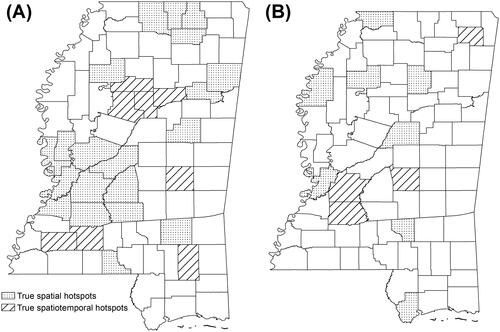
A small-scale Monte Carlo simulation study was conducted to assess the validity of the proposed model in predicting the suppressed values as well as identifying true spatial hot spots and state- and county-level trends. The template used for the simulation is the boundaries of the eighty-two counties in Mississippi, which is also the one used in the empirical study that follows. We simulated data sets from the proposed model in two different scenarios (Figure 1). First, counties with truly elevated S_is (twenty out of eighty-two, ∼25 percent) and δ_is (eight out of eighty-two, ∼10 percent) cluster in different sizes (i.e., large, small, and singleton; Figure 1A). Second, fewer counties (compared with the former scenario) have truly elevated S_is and δ_is (eight and four out of eighty-two, respectively), which were randomly selected and most were located as singletons (Figure 1B). In both scenarios, the mean vector for S_is and δ_is was a piecewise constant. The mean for counties with truly elevated S_is or δ_is was 1 and for the remaining counties, the mean was 0. For each scenario, data were generated for three different types of spatial autocorrelations: (1) independence (${\rho }_s^{},$ ${\rho }_{\delta }^{}$ = 0), (2) moderate spatial dependence (${\rho }_s^{},$ ${\rho }_{\delta }^{}$ = 0.5), and (3) strong spatial dependence (${\rho }_s^{},$ ${\rho }_{\delta }^{}$ = 0.95). For simplicity, we set the expected count to five for all counties because we used five as the cutoff value for data suppression in the simulation. The global trend $\beta$ was set as −0.1 (i.e., a decreasing trend). This setting, together with the setting for expected counts, allows the number of suppressed values in the simulated data set to be comparable to that in the empirical data set in Mississippi. The maximum and minimum numbers of counties with suppressed values were sixty-eight and eighteen (out of eighty-two), respectively, in the simulated data set. A value of 0.1 was set for ${\sigma }_s^{}$ and ${\sigma }_{\delta }^{}.$ Also for simplicity, time t* was the only covariate used in the simulation, and α, ϕ_t, and ξ_it were set as 0. One hundred data sets were simulated for each combination of the scenario and the type of spatial autocorrelation. This number of simulations reduces computation time but allows the average statistics over simulated data sets to be representative (Hossain and Lawson 2010). A total of 600 data sets were generated and analyzed.

Figure 1 Counties with truly elevated S_i (i.e., spatial hot spots, stippled) and δ_i (i.e., spatiotemporal hot spots, hatched) in two different scenarios.

Results from the Simulation Study

The performance of the proposed model in estimating the regression coefficient (β) as well as in detecting true spatial and spatiotemporal hot spots is presented in Table S.1 in the Supplemental Material. Results indicate that the model estimates β reasonably well in different scenarios with different levels of spatial autocorrelation. The proposed model also performs well in detecting true spatial and spatiotemporal hot spots, especially in correctly identifying true hot spots (i.e., high sensitivity values). Generally, using an increasingly conservative cutoff c (i.e., from 0.80–0.99), sensitivity values decrease and specificity values increase. When the commonly accepted cutoff of 0.80 is used, a notable percentage of counties are falsely detected as hot spots, especially in the cases when moderate or strong spatial dependence is present in the data set or when the hot spots are singletons (in particular singleton spatiotemporal hot spots in Scenario 2), probably attributable to the uncertainties introduced by data suppression. Therefore, a more conservative value of the cutoff c, for example, 0.95 or 0.99, should be used to detect true hot spots or cold spots from data sets with suppressed values. To balance sensitivity and specificity, we use a cutoff 0.95 in analyzing Mississippi’s new HIV diagnosis and PrEP use data sets. The proposed model also imputes the suppressed values well. As expected, the posterior distributions of imputed values cover the true value. In most cases, the suppressed values are likely to be imputed with the true value or a value immediately next to the true value. Figure S.1 in the Supplemental Material shows a selection of imputations for suppressed values, with gray bars representing the posterior probability distributions of imputed values and the red vertical lines representing the true values.

Table 1. Cross-classification based on a county’s hot spot or cold spot status of new HIV diagnoses and PrEP use

	New HIV diagnoses			PrEP use			Counties
	Hot spot	Cold spot	Neither	Hot spot	Cold spot	Neither
Category 1	✖			✖			Hinds, Madison, Warren, Rankin, Copiah, Harrison
Category 2	✖				✖		Lee
Category 3	✖					✖	Washington, Bolivar, Leflore, Pike, Forrest, Coahoma
Category 4		✖		✖			Jackson
Category 5		✖			✖		Prentiss, Tishomingo
Category 6		✖				✖	Pearl River, Pontotoc, Union, Tippah, Itawamba
Category 7			✖	✖			Lawrence, Simpson, Hancock
Category 8			✖		✖		Alcorn
Category 9			✖			✖	Others

Note: PrEP = pre-exposure prophylaxis.

Study Region and Data

Study Region: Mississippi, United States

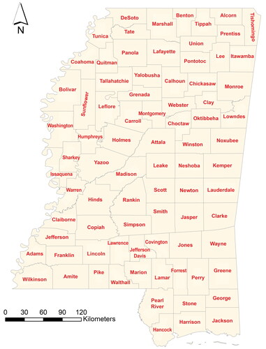
Our study region is Mississippi, one of the southern states with the highest HIV rates in the United States. Mississippi was also prioritized by the EHE plan in its first phase with additional resources to implement locally tailored initiatives. Mississippi has the eighth and sixth highest rates of HIV diagnosis among adults and AIDS diagnosis, respectively, in the country (Mississippi State Department of Health 2021). In 2018, the rate of people who live with HIV was 381 per 10,000 population. Conversely, PrEP use rate and PnR in Mississippi are among the lowest in the United States. In the fourth quarter of 2017, the state’s PnR was the second lowest among all states (Siegler, Bratcher, et al. 2018). In total, there are eighty-two counties in Mississippi (Figure 2).

Figure 2 Mississippi state and county boundaries.

New HIV Diagnoses and PrEP Use in Mississippi, 2014–2018

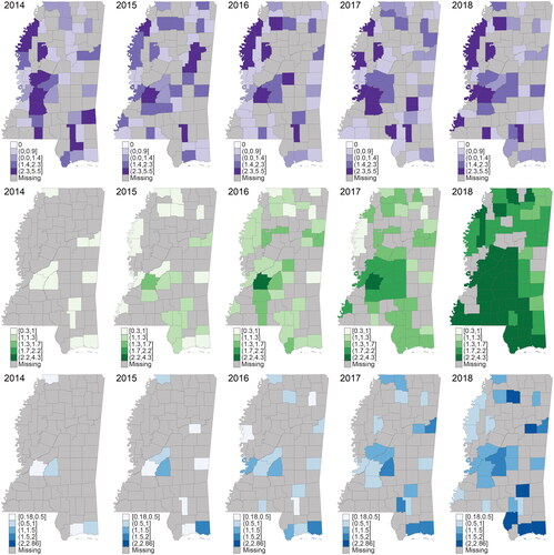
We obtained county-level annual counts of new HIV diagnoses and PrEP users as well as crude PnR in Mississippi between 2014 and 2018 from AIDSVu. The counts of new HIV diagnoses in the range [1, 4] and PrEP users less than three are suppressed. Annual population data from 2014 to 2018 were retrieved from the American Community Survey (ACS) five-year estimates. New HIV diagnoses per 10,000 population, PrEP use per 10,000 population, and crude PnR are shown in Figure 3. Suppressed values are mapped as “missing” in gray. No obvious changes are observed for new HIV diagnoses in Mississippi during the study period. Counties with a higher new HIV diagnosis rate locate in the central and northwest areas including the Jackson Metropolitan Area. The number and the patterns of counties with one to four new HIV diagnoses (thus suppressed) were stable during the study period. In contrast, there was an apparent increasing trend of PrEP use in Mississippi, indicated by fewer counties with zero to two PrEP users as well as higher PrEP use prevalence over the years. PrEP use rates in central and southern counties were higher than those in northern counties. Regarding crude PnR, because either suppressed or zero new HIV diagnoses or suppressed PrEP user counts led to suppressed PnR, a substantial percentage of counties’ PnR values were not publicly released by AIDSVu. An increasing trend of PnR, however, is observed given higher minimum and maximum PnR values across the study period. Descriptive statistics of new HIV diagnoses and PrEP use in Mississippi, including the number of counties with suppressed values over time, are provided in Table S.2 in the Supplemental Material. We first fitted Model A (without covariates) to the Mississippi data sets.

Figure 3 High proportions of suppressed values (shaded areas) in new HIV diagnosis and pre-exposure prophylaxis (PrEP) use in Mississippi, 2014–2018, using publicly accessible data from AIDSVu. First row: New HIV diagnoses per 10,000 population. Second row: Pre-exposure prophylaxis (PrEP) use per 10,000 population. Third row: Crude PrEP-to-need ratio (PnR).

Social Determinants of Health Variables

We extended Model A to Model B by incorporating four variables on social determinants of health (SDH) known to be associated with HIV and PrEP use (Gant et al. 2012; An et al. 2013; Jeffries and Henny 2019; Ransome et al. 2020), thus helping explain the spatiotemporal patterns identified in Model A. The SDH variables include socioeconomic deprivation (i.e., a composite index derived from median household income, percentage of population living in poverty, percentage of population with less than a high school education, and percentage of population unemployed using principal component analysis), income inequality (i.e., Gini coefficient), percentage of population without health insurance, and residential segregation that uses the percentage of Black population as a proxy (Ransome et al. 2016). The SDH variables were measured at a five-year lag from the new HIV diagnosis and PrEP use data and retrieved from ACS five-year estimates (e.g., 2010–2014 ACS data for new HIV diagnosis and PrEP use in 2014).

Results

Model Diagnostics

Three (out of 201 counties with unsuppressed values, 1.5 percent) and zero (out of 188 counties with unsuppressed values) had a PPP value outside the range between 0.05 and 0.95 for the counts of new HIV diagnoses and PrEP users, respectively. Those results suggest that our model fitted the observed data set fairly well. In other words, the replicated data resembled the observed data. This resemblance is further illustrated by Figure S.2 in the Supplemental Material, which shows that all the observed number of new HIV diagnoses or PrEP users were within the 95 percent CrI of the predicted samples. No misprediction patterns (i.e., more likely to occur at a particular location, time point, or both) were observed for the three counties with a PPP value greater than 0.95 or smaller than 0.05.

All the imputed values for suppressed counts of new HIV diagnoses and PrEP users fall within their corresponding possible ranges (i.e., [1, 4] and [0, 2], respectively). Figure S.3 in the Supplemental Material shows the posterior density plots of 20,000 samples of the estimated counts for four randomly selected counties where their values were suppressed for one or more years (Bolivar, Stone, Tate, and Lafayette). It indicates that all possible values for the suppressed numbers of new HIV diagnoses and PrEP users were sampled such that the uncertainty associated with the imputation was accounted for in posterior statistical inferences.

Main Spatial Patterns of New HIV Diagnoses and PrEP Use

Figure 4 shows the model estimates of the main spatial patterns of new HIV diagnoses and PrEP use in Mississippi. According to Figure 4A1, counties in central and northwest Mississippi constantly had a higher risk of new HIV diagnosis during the study time period (exp($S_i^{k=1}$) > 1, two darker categories), whereas other areas, in particular the northeastern part of the state, had a lower risk (exp($S_i^{k=1}$) < 1). To account for the uncertainty associated with the posterior mean (PM) in Figure 4A1, we also map the PP of a county with higher risk of new HIV diagnosis (i.e., PP(exp($S_i^{k=1}$) > 1)). Based on our simulation study, a conservative value of the cutoff c, 0.95, was chosen to detect hot spots and cold spots from data sets with suppressed values. A PP value greater than 0.95 suggests strong evidence that the corresponding county has elevated new HIV diagnosis risk (i.e., hot spot), whereas a PP value smaller than 0.05 indicates a lower risk (i.e., cold spot). Figure 4A2 shows that new HIV diagnosis hot spots (i.e., darkest category) located in central, northwestern, and small pockets of areas in Mississippi, whereas cold spots clustered in the northeast and were scattered across the study region.

Figure 4 Main spatial patterns of new HIV diagnosis and pre-exposure prophylaxis (PrEP) use. (A1) Posterior mean (PM) of new HIV diagnosis risk (exp($S_i^{k=1}$)). (A2) Posterior probability (PP) of having a higher risk (PP(exp($S_i^{k=1}$) > 1)). (B1) PM of PrEP use (exp($S_i^{k=2}$)). (B2) PP of having a higher PrEP use (PP(exp($S_i^{k=2}$) > 1)). Ceased hot spots and cold spots cross-hatched in yellow; new hot spots stippled; new cold spots hatched in black.

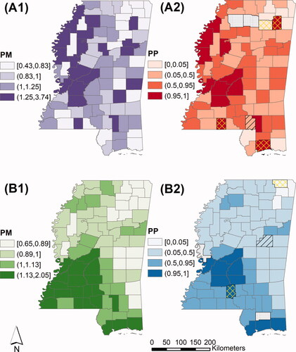
A distinct spatial pattern of PrEP use was detected in Mississippi. Southern and southwestern counties tended to have a higher rate of PrEP use (i.e., exp($S_i^{k=2}$) > 1) than their eastern and northern counterparts (Figure 4B1). Accounting for the uncertainties with PM, Figure 4B2 shows the PP of a county with a higher PrEP use. All PrEP use hot spots (i.e., PP(exp($S_i^{k=2}$) > 1) > 0.95) were located in central and southern Mississippi and most cold spots of PrEP use (i.e., PP(exp($S_i^{k=2}$) > 1) < 0.05) were located in the northeast.

The inclusion of SDH variables helped explain some hot spots and cold spots of new HIV diagnoses and PrEP use (cross-hatched in yellow in Figure 4A2 and 4B2), but most of them remained unexplained. There were, however, a small number of counties that became hot spots (stippled) and cold spots (hatched in black) after incorporating SDH variables, possibly attributable to the interactions among covariates or covariates’ spatially varying effects that were not accounted for (Haining and Li 2020).

State-Level Main Temporal Trends of New HIV Diagnoses and PrEP Use

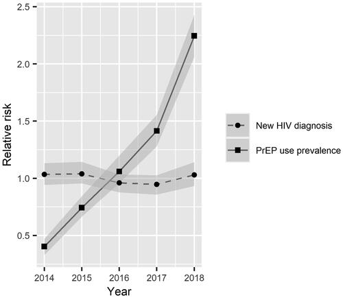
State-level main temporal trends of new HIV diagnoses and PrEP use (i.e., trends of the two outcomes at the state level in Mississippi) are shown in Figure 5. There was no statistically significant temporal trend (increasing or decreasing) of new HIV diagnoses in Mississippi between 2014 and 2018 given that the 95 percent CrI of ${\beta }_{}^{k=1}$ covered zero (PM: −0.01, 95% CrI: [–0.12, 0.10]) and the main temporal risk of new HIV diagnoses (i.e., exp(${\beta }_{}^{k=1}{t}^{*}+{\varphi }_t^{k=1}$)) across all years covered one. Conversely, ${\beta }_{}^{k=2}$significantly differed from zero (PM: 0.41, 95% CrI: [0.22, 0.61]) and the 95 percent CrI of temporal PrEP use (i.e., exp(${\beta }_{}^{k=2}{t}^{*}+{\varphi }_t^{k=2}$)) were away from one, suggesting there was a sharp, statistically significant increasing trend of PrEP use in Mississippi during the study period, particularly between 2017 and 2018.

Figure 5 State-level main temporal trends of new HIV diagnoses (stable) and pre-exposure prophylaxis (PrEP) use (sharply increasing) in Mississippi (exp(${\beta }_{}^k{t}^{*}+{\varphi }_t^k$)), 2014–2018.

County-Level Departure Trends of New HIV Diagnoses and PrEP Use

County-level departures of new HIV diagnoses and PrEP use from the corresponding state-level trends in Mississippi are shown in Figure 6. Looking at Figure 6A1 and 6B1 (i.e., PM of ${\delta }_i^k$), all counties departed, either in a positive (${\delta }_i^k$ > 0) or negative (${\delta }_i^k$ < 0) manner, from state-level trends of new HIV diagnoses and PrEP use. This point estimate, however, had a high level of uncertainty. Mapping the PP of a positive ${\delta }_i^k$ (Figure 6A2 and 6B2) reveals that none of the departures were statistically significant. For new HIV diagnoses (Figure 6A2), however, there was moderate evidence that the trend in DeSoto County in the north positively departed from the state-level trend (i.e., increasing trend compared with state-level trend, PP(${\delta }_i^{k=1}$ > 0) = 0.80). 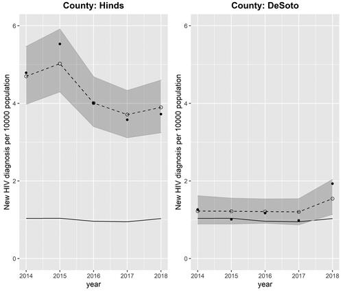Hinds County, where the Jackson Metropolitan Area is located, showed some evidence of a decreasing trend of new HIV diagnoses compared with the state-level trend (i.e., PP(${\delta }_i^{k=1}$ > 0) = 0.19). County-specific trends of new HIV diagnoses in DeSoto and Hinds counties are depicted in Figure 7 in dashed lines, which differ from the state-level trend shown in solid lines.

Figure 6 County-level departure trends of new HIV diagnoses and pre-exposure prophylaxis (PrEP) use from state-level trends in Mississippi (${\delta }_i^k$): (A1) Posterior mean (PM) of ${\delta }_i^{k=1}.$ (A2) Posterior probability (PP) of having a positive ${\delta }_i^{k=1}.$ (B1) PM of ${\delta }_i^{k=2}.$ (B2) PP of having a positive ${\delta }_i^{k=2}.$

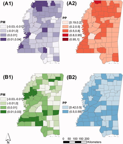
Figure 7 Temporal trends of new HIV diagnosis in Hinds and DeSoto counties, 2014–2018. Solid point: observed new HIV diagnosis rate per 10,000 population; circle: predicted new HIV diagnoses per 10,000 population; gray region: 95 percent CrI of predicted new HIV diagnosis rate; dashed line: predicted county-specific trend of new HIV diagnoses; solid line: state-level trend of new HIV diagnosis.

Comparatively, no counties’ trend in PrEP use markedly differed from state-level trend between 2014 and 2018 (Figure 6B2). All the PPs of a county with a positive ${\delta }_i^{k=2}$ (i.e., PP(${\delta }_i^{k=2}$ > 0)) fell between 0.42 and 0.59. It suggests that all counties in Mississippi had an increasing trend in PrEP use, similar to the state-level trend (as shown in Figure 5). None of them had a faster or slower pace. Accounting for SDH variables did not help explain the variations in ${\delta }_i^k.$ Hinds and DeSoto remained the counties with the lowest (0.23) and highest (0.72) PP(${\delta }_i^{k=1}$ > 0), respectively. Therefore, we map the patterns from the unadjusted Model A only.

Further Examination of Counties Based on New HIV Diagnoses, PrEP Use, and PnR

Overlapping Figure 4A2 and 4B2, we further classify the counties in Mississippi into different categories based on whether a county was a new HIV diagnosis/PrEP use hot spot or cold spot. The classification rules and identified counties in each category are presented in Table 1 and mapped in Figure 8. Some counties such as Hinds County constantly experienced elevated rates of new HIV diagnosis during the study period, but in parallel with higher PrEP use (i.e., Category 1), whereas others had lower new HIV diagnosis rate as well as lower PrEP use (i.e., Category 5 including Prentiss County). The best scenario is lower new HIV diagnosis rate coupled with higher PrEP use (i.e., Category 4), with only one county identified (Jackson). Counties that potentially warrant special attention are those with higher rates of new HIV diagnosis but lower PrEP use (Category 2; i.e., Lee County).

Figure 8 County classification based on hot spot/cold spot status of new HIV diagnoses and pre-exposure prophylaxis (PrEP) use. The colored dots represent PrEP-to-need ratio (PnR) hot spot or cold spot status in 2018.

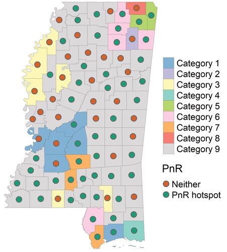
Although cross-classifications (Table 1) provide useful insights into new HIV diagnoses and PrEP use, separately, in each county, they are less informative regarding the relative relationship between HIV burden and PrEP use and coverage. For example, for counties belonging to Category 1 with both elevated new HIV diagnoses and PrEP use, does PrEP use meet the need of HIV prevention? We therefore further examine counties in Mississippi by accounting for the estimated PnR in 2018. A PP(PnR > 1) greater than 0.95 indicates strong evidence that the number of PrEP users in a county exceeds the number of new HIV diagnoses (i.e., hot spot), whereas a PP(PnR > 1) < 0.05 suggests otherwise (i.e., cold spot; Figure 8). A PP(PnR > 1) value between 0.05 and 0.95 indicates neither a hot spot nor a cold spot. The full picture of estimated PnR in Mississippi during the study period is mapped in Figure S.4 in the Supplemental Material. Based on the cutoff c = 0.95, no PnR cold spots were identified. This is not surprising given that PrEP use sharply increased whereas new HIV diagnoses remained stable during the study period. Consistent findings of PnR were identified for Categories 2 through 9. For example, when a county was a new HIV diagnosis cold spot, no matter if it was a hot spot, cold spot, or neither of PrEP use (Categories 4, 5, and 6), its PP(PnR > 1) was always greater than 0.95 in 2018. In contrast, mixed findings of PnR were found in Category 1. When a county was a hot spot of both new HIV diagnosis and PrEP use, it could be either a PnR hot spot (e.g., Madison County, PP(PnR > 1) = 0.99) or neither PnR hot spot nor cold spot (e.g., Hinds County, PP(PnR > 1) = 0.76).

Associations between New HIV Diagnoses/PrEP Use and SDH Variables

Among the four SDH variables included to account for the spatiotemporal variations in new HIV diagnoses and PrEP use, only socioeconomic deprivation had a statistically significant (i.e., the 95 percent CrI does not cover one) and positive association with new HIV diagnoses (Table 2). That is also why only a small number of hot spots and cold spots were explained by the inclusion of SDH variables, as shown in Figure 4. With one unit increase in socioeconomic deprivation, there was a 45 percent increase in new HIV diagnoses.

Table 2.  The associations between new HIV diagnoses, pre-exposure prophylaxis (PrEP) use, and social determinants of health variables

	New HIV diagnosis	PrEP use
Socioeconomic deprivation	1.45 [1.19, 1.75]	1.06 [0.93, 1.19]
Income inequality	0.92 [0.82, 1.03]	0.99 [0.92, 1.08]
Percentage of population without health insurance	0.88 [0.76, 1.02]	0.96 [0.87, 1.05]
Residential segregation	0.95 [0.80, 1.12]	1.02 [0.93, 1.12]

Note:: Posterior mean (PM) followed by 95 percent credible interval in brackets. Statistically significant coefficients are shown in bold.

Discussion

Using a Bayesian statistical model to analyze openly accessible county-level censored data sets, our study uncovered detailed spatiotemporal patterns of new HIV diagnoses and PrEP use in Mississippi between 2014 and 2018. The main spatial pattern indicates that across the study period, hot spots of new HIV diagnosis clustered in central and northwestern Mississippi and cold spots were located in northeastern and southern counties. This finding generally aligns with a previous study (Stopka et al. 2018), where the authors analyzed new HIV diagnoses, spatially rather than spatiotemporally, in Mississippi at the census tract level using aggregated data between 2008 and 2014. This alignment corroborates our findings that the trend of new HIV diagnoses remained stable at the state level (not statistically significantly increasing or decreasing) during the study period, and most counties followed this main temporal trend except Hinds and DeSoto counties. This insignificant main temporal trend of new HIV diagnosis in Mississippi is also consistent with the reported stable HIV incidence at the national level between 2014 and 2018 (CDC 2020). As for PrEP use, the main spatial pattern reveals that central and southern urban Mississippi constantly had higher rates of PrEP use than northern rural areas during the study period, which is consistent with a previous finding (Siegler et al. 2020). The entire state and all counties in Mississippi had a similar sharp increase in PrEP use from 2014 to 2018, echoing existing state- and county-level PrEP use studies for the entirety of the United States (Sullivan et al. 2018; Mouhanna et al. 2020).

Our research highlights the importance of using a relative measure of PrEP use. Looking at new HIV diagnosis and PrEP use separately, counties in Category 2 (Table 1) seem to warrant particular attention given that they were identified as new HIV diagnosis hot spots and PrEP use cold spots. PrEP use, however, has increased sharply such that a county with relatively lower PrEP use compared with other counties in the state can meet its HIV prevention need. As illustrated, counties in Category 2 were not necessarily PnR cold spots. Conversely, even if a county has a high (absolute) number of PrEP users, it is not guaranteed to be a PnR hot spot due to its concurrently high number of new HIV diagnoses. Although HIV interventions should be prioritized for counties identified as spatial hot spots of new HIV diagnosis (i.e., counties with constantly higher risks over time), special attention is needed for DeSoto County. It was not identified as a new HIV diagnosis hot spot and was detected as a PnR hot spot. There was evidence, however, that its trend in new HIV diagnoses was positively departing from the stable state-level trend, but its trend in PrEP use did not outpace the state-level trend. If DeSoto’s trends in new HIV diagnoses and PrEP use continue, it could become a new hot spot of new HIV diagnoses and stop being a PnR hot spot.

The positive association between new HIV diagnoses and socioeconomic deprivation identified in Mississippi is consistent with findings from previous studies across U.S. counties (An et al. 2013) and other local cities (e.g., New York City; Ransome et al. 2016). Our findings from Mississippi underscore previous theoretical evidence that structural factors such as inequality and poverty are key to addressing HIV disparities (Buot et al. 2014; Sullivan et al. 2021). Although disentangling the associations between new HIV diagnoses and PrEP use and SDH is not the focus of this study, further research is needed to understand why some SDH variables (i.e., inequality income, percentage of population without health insurance, and residential segregation) had marginal impacts on the HIV and PrEP outcomes in this region at the county level. Indeed, other studies (albeit in Catalonia, Spain; Agustí et al. 2020) have shown that social determinants like economic deprivation are inconsequential to new HIV diagnosis in the presence of other factors such as proportion of gay and bisexual men who have sex with men (MSM), but those results may be context and country dependent. There could, however, be alternative explanations for these findings; for example, the spatial scale (e.g., census tracts rather than counties, part of the modifiable areal unit problem), time lag between new HIV diagnoses and PrEP use and SDH variables (three-year rather than five-year lag), and demographic stratification (data stratified by race or ethnicity rather than aggregated for all races and ethnicities) all affect the statistical significance. Future work should consider including other explanatory variables, such as access to HIV screening, health literacy, transportation barriers, and access to tele-medicine technology into the model to help explain the remaining spatiotemporal variations in HIV and PrEP use (Sullivan et al. 2021).

Several strengths of our study should be highlighted. First, it uses a Bayesian spatiotemporal statistical model to analyze interval- and left-censored data sets. The simulation study has demonstrated its robustness in identifying hot spots and cold spots as well as regression coefficients in different scenarios. Furthermore, the model predicts the unsuppressed counts reasonably well, irrespective of whether the count is large or small (e.g., the number of new HIV diagnoses ranges between 0 and 118 during the study period). It also predicts the censored values within the possible ranges. Compared with traditional methods that have been used to analyze publicly accessible data with a high proportion of suppressed values (e.g., deleting the missing data from the analysis), our approach retains all available information (i.e., the suppressed values lie between a known interval) for statistical inferences. This added strength makes our findings more robust and reliable to help public health departments allocate their resources with confidence. Our approach also outperforms commonly used imputation methods based on frequentist methods due to its capacity of propagating and quantifying uncertainties (via posterior probabilities) by using the Bayesian framework. This feature is particularly captivating given the (probably high) uncertainties introduced by data suppression.

Second, our study provides an estimated measure of PnR, which overcomes some limitations associated with crude PnR calculations. In particular, our method “borrows” information from neighboring counties and years, and uses imputed values from the censored probability distributions. Compared with the crude PnR, the estimated PnR is less vulnerable to the small number problem (the number of new HIV diagnoses and PrEP users of a county are usually low) due to the smoothing effect of information borrowing (Law, Quick, and Chan 2015). An important caveat with smoothing is that it reduces the variance of estimated values, and therefore can possibly lead to oversmoothed PnR values (Best, Richardson, and Thomson 2005) such that the estimates are not representative of the true values, imposing challenges of identifying the underlying patterns. Given that PrEP use is spatially continuous and autocorrelated (the correlation parameter estimated from the Leroux prior in Model A is 0.49), and not restricted to residential counties (Sullivan et al. 2021), it is reasonable to pool information from neighboring counties to smooth the estimated PnR values toward the local mean value. Unfortunately, it is infeasible in our study to quantify how well the smoothing effect estimated from the data aligns with PrEP use in reality. Moreover, our method provides PnR estimates for counties where the counts of new HIV diagnoses or PrEP users were suppressed, or where zero new HIV diagnoses were observed, along with uncertainty measures including the 95 percent CrI. For example, the estimated PnR for Yalobusha County, where all the counts of new HIV diagnoses and PrEP users were suppressed, were 0.21, 0.40, 0.61, 0.82, and 1.19, respectively, between 2014 and 2018 after accounting for SDH variables. An increasing trend of estimated PnR was estimated in this and other counties where crude PnR were suppressed, which aligns with our general findings in this study. These estimates allow the ranking and comparison of PnR across counties with suppressed crude PnR values, which could be informative for prioritizing interventions in these areas. It would be ideal, though, to examine whether and how the estimated PnR deviates from the crude PnR if the raw, unsuppressed data are accessible.

Third, we used objective PrEP use data from pharmacy records such that self-reporting bias is reduced (Mouhanna et al. 2020). Finally, our study examined the spatiotemporal patterns of new HIV diagnosis and PrEP at the county rather than state level, from which the results are informative for allocating resources and implementing locally tailored HIV interventions. Although crude HIV incidence suggested that there was a 12 percent increase in new HIV diagnoses in Mississippi from 2017 to 2018 (Mississippi State Department of Health 2021), our results indicate that new HIV diagnoses remained stable at the state level and in most counties. This crude rate increase could be attributed to notable increases of new HIV diagnosis within a small number of counties, in particular those with an increasing trend compared with the state-level stable trend. In our case, it is DeSoto County, which had seventeen and thirty-four new HIV diagnosis cases in 2017 and 2018, respectively; therefore, HIV prevention resources should be targeted to that area.

Our research can be extended in several directions. First would be analyzing race and ethnicity stratified HIV and PrEP use data sets. The HIV epidemic in Mississippi is racially disproportionate. Black Mississippians, who make up 37.4 percent of the state’s population, accounted for 76 percent of new HIV diagnoses in 2018 (Mississippi State Department of Health 2021). Our proposed model is highly appropriate to examine race- and ethnicity-specific spatiotemporal patterns of new HIV diagnosis, PrEP use, and PnR because race and ethnicity data are often incomplete. Having a way to reliably estimate race- and ethnicity-specific estimates will be more informative for implementing interventions aiming to end the epidemic. Further stratification based on specific demographic characteristics potentially leads to higher levels of data suppression or zero-inflation, thus requiring more sophisticated statistical modeling approaches. Second, the PnR threshold used to detect hot spots and cold spots should be further examined. We used PnR > 1 as the threshold, with the assumption that a PnR smaller than one indicates unmet need in HIV prevention in a specific county. Therefore, addressing PrEP use in this county is particularly important. People who use PrEP might not be the ones who need it most, however (i.e., most vulnerable populations including MSM). Future studies should evaluate whether a more conservative threshold is needed, for example, with a PnR greater than two (i.e., PP(PnR > 2) > 0.95), the ratio level at which PrEP is effective in reducing HIV infections. Third, new HIV diagnoses and PrEP use over a longer period (i.e., more than five years) should be analyzed to better surveil the evolution of these two phenomena in Mississippi when more recent data become available. Although the models applied in our study provide robust trend estimates with uncertainties quantified via the 95 percent CrI, they are suitable only for short time series data with a few time points (e.g., two to five) and become restrictive when data observed at more time points are analyzed. Therefore, mixture models characterizing the probability of a county-level trend departing from a state-level trend should be used (Li et al. 2012; Boulieri, Bennett, and Blangiardo 2020). Fourth, our proposed approach is theoretically scalable to thousands or more spatiotemporal analysis units so it can be applied in a larger geographical extent or finer spatial scale with more observations. Implementing the proposed Bayesian models with MCMC algorithms for a bigger data set, however, will be much more computationally challenging, attributable to the necessity of dealing with the n × n covariance matrix (n is the number of spatial units) at each iteration as well as estimating the (sometimes dramatically) increasing number of parameters. Although model convergence took over 30 minutes and 150 hours, respectively, for the empirical Mississippi data set and the 600 simulated data sets (410 = 82 * 5 analysis units in total) by running on a desktop with decent configurations,¹ we anticipate a much slower and more time-consuming process when a bigger data set is fitted. Finally, local adaptive priors that account for potential abrupt changes in new HIV diagnoses and PrEP use between adjacent counties (e.g., Lee and Mitchell 2013; Corpas-Burgos and Martinez-Beneito 2020; Dong et al. 2020) can be applied in the analysis for other study settings or spatial scales. We fitted a locally adaptive model following Corpas-Burgos and Martinez-Beneito (2020) because of its feasibility of model implementation in BUGS language using NIMBLE. Yet the model failed to converge probably because the model proposed in this study has sufficiently captured the spatiotemproal variations in new HIV diagnosis and PrEP use in Mississippi. In addition, as shown in the simulation study, the proposed model performs well in detecting singleton hot spots if a conservative value of cutoff c is used. County-level or local abrupt changes in HIV and PrEP use are worth examining in other contexts though.

Conclusion

This study contributes to the literature by applying a Bayesian spatiotemporal model to address the data suppression issue inherent in publicly accessible HIV and PrEP use data at the county level that, if not accurately handled, could delay achieving the EHE goals of eliminating HIV by 2030. To the best of our knowledge, our study is also the first that uses a robust spatial statistical approach to jointly model the dynamics of PrEP use and new HIV diagnoses. We showed the power of using Bayesian spatiotemporal models to address the data suppression issue and incorporate all available information for statistical inferences, which allows us to see a full picture of HIV burden and PrEP use in areas like Mississippi, thus benefiting health interventions. The results reveal that our model provides greater geographic coverage of HIV and PrEP use estimates with public data sets and can identify counties that appear to deviate from the global state-level trends. Our findings of spatiotemporal variations of new HIV diagnosis and PrEP use in Mississippi are informative for identifying counties that should be prioritized for allocating state-level funding from EHE, the federal initiative that targets funding to specific counties with high HIV burdens.

Acknowledgments

We would like to thank our editor, Dr. Ling Bian, and three anonymous referees for their insightful feedback that helped improve this article.

Supplemental Material

Supplemental data for this article can be accessed on the publisher’s site at: http://dx.doi.org/10.1080/24694452.2022.2080040. Included are detailed descriptions of using exceedance probabilities to detect hot spots and cold spots and model comparisons by specifying different priors to $S_i^k$ and ${\delta }_i^k.$ Additional results from analyzing simulated and empirical data sets are also included.

Additional information

Notes on contributors

Hui Luan

HUI LUAN is an Assistant Professor in the Department of Geography, University of Oregon, 1251 University of Oregon, Eugene, OR 97403-1251. E-mail: [email protected]. His research focuses on Bayesian spatial and spatiotemporal modeling and its applications in exploring inequities of urban environmental exposures and their associations with health.

Yusuf Ransome

YUSUF RANSOME is an Assistant Professor in Social and Behavioral Sciences, Yale School of Public Health, 60 College Street, New Haven, CT 06520. E-mail: [email protected]. His research investigates how social, economic, and cultural determinants influence racial, ethnic, and geography-related disparities in HIV care continuum indicators and alcohol use disorders.

Notes

1 Dell Precision 5820 Tower, 64-bit Windows operating system, 32GB RAM, and Intel Xeon W-2123 CPU @ 3.60 GHz.

References

- Agustí, C., N. Font-Casaseca, F. Belvis, M. Julià, N. Vives, A. Montoliu, J. M. Pericàs, J. Casabona, and J. Benach. 2020. The role of socio-demographic determinants in the geo-spatial distribution of newly diagnosed HIV infections in small areas of Catalonia (Spain). BMC Public Health 20 (1):1–10. doi: 10.1186/s12889-020-09603-7.
- Amram, O., J. Shoveller, R. Hogg, L. Wang, P. Sereda, R. Barrios, J. Montaner, and V. Lima. 2018. Distance to HIV care and treatment adherence: Adjusting for socio-demographic and geographical heterogeneity. Spatial and Spatio-Temporal Epidemiology 27:29–35. doi: 10.1016/j.sste.2018.08.001.
- An, Q., J. Prejean, K. M. D. Harrison, and X. Fang. 2013. Association between community socioeconomic position and HIV diagnosis rate among adults and adolescents in the United States, 2005 to 2009. American Journal of Public Health 103 (1):120–26. doi: 10.2105/AJPH.2012.300853.
- Bartell, S. M., and T. A. Lewandowski. 2011. Administrative censoring in ecological analyses of autism and a Bayesian solution. Journal of Environmental and Public Health 2011:1–5. doi: 10.1155/2011/202783.
- Besag, B. J. 1974. Spatial interaction and the statistical analysis of lattice systems. Journal of the Royal Statistical Society: Series B 36 (2):192–236.
- Besag, J., J. York, and A. Mollie. 1991. Bayesian image restoration, with two applications in spatial statistics. Annals of the Institute of Statistical Mathematics 43 (1):1–20. doi: 10.1007/BF00116466.
- Best, N., S. Richardson, and A. Thomson. 2005. A comparison of Bayesian spatial models for disease mapping. Statistical Methods in Medical Research 14 (1):35–59.
- Blangiardo, M., A. Boulieri, P. Diggle, F. B. Piel, G. Shaddick, and P. Elliott. 2020. Advances in spatiotemporal models for non-communicable disease surveillance. International Journal of Epidemiology 49 (Suppl. 1):I26–I37. doi: 10.1093/ije/dyz181.
- Boulieri, A., J. E. Bennett, and M. Blangiardo. 2020. A Bayesian mixture modeling approach for public health surveillance. Biostatistics 21 (3):369–83. doi: 10.1093/biostatistics/kxy038.
- Buot, M. L. G., J. P. Docena, B. K. Ratemo, M. J. Bittner, J. T. Burlew, A. R. Nuritdinov, and J. R. Robbins. 2014. Beyond race and place: Distal sociological determinants of HIV disparities. PLoS ONE.9 (4):e91711. doi: 10.1371/journal.pone.0091711.
- Centers for Disease Control and Prevention (CDC). 2020. Estimated HIV incidence and prevalence in the United States, 2014–2018. HIV Surveillance Supplemental Report 25 (1). Accessed May 27, 2021. https://www.cdc.gov/hiv/pdf/library/reports/surveillance/cdc-hiv-surveillance-supplemental-report-vol-25-1.pdf.
- Corpas-Burgos, F., and M. A. Martinez-Beneito. 2020. On the use of adaptive spatial weight matrices from disease mapping multivariate analyses. Stochastic Environmental Research and Risk Assessment 34 (3–4):531–44. doi: 10.1007/s00477-020-01781-5.
- Dong, G., J. Ma, D. Lee, M. Chen, G. Pryce, and Y. Chen. 2020. Developing a locally adaptive spatial multilevel logistic model to analyze ecological effects on health using individual census records. Annals of the American Association of Geographers 110 (3):739–57. doi: 10.1080/24694452.2019.1644990.
- Duncan, E. W., N. M. White, and K. Mengersen. 2017. Spatial smoothing in Bayesian models: A comparison of weights matrix specifications and their impact on inference. International Journal of Health Geographics 16 (1):47. https://ij-healthgeographics.biomedcentral.com/articles/. doi: 10.1186/s12942-017-0120-x.
- Elmore, K., E. L. P. Bradley, A. C. Lima, G. M. Khalil, E. Obi-Tabot, Z. Gant, H. D. Dean, and D. H. McCree. 2019. Trends in geographic rates of HIV diagnoses among black females in the United States, 2010–2015. Journal of Women’s Health 28 (3):410–17. doi: 10.1089/jwh.2017.6868.
- Fauci, A. S., R. R. Redfield, G. Sigounas, M. D. Weahkee, and B. P. Giroir. 2019. Ending the HIV epidemic: A plan for the United States. JAMA 321 (9):844–45. doi: 10.1001/jama.2019.1343.
- Fridley, B. L., and P. Dixon. 2007. Data augmentation for a Bayesian spatial model involving censored observations. Environmetrics 18 (2):107–23. doi: 10.1002/env.806.
- Gant Z., M. Lomotey, H. I. Hall, X. Hu, X. Guo, and R. Song. 2012. A county-level examination of the relationship between HIV and social determinants of health: 40 states, 2006–2008. The Open AIDS Journal 6 (1):1–7. doi: 10.2174/1874613601206010001.
- Gelman, A. 2006. Prior distribution for variance parameters in hierarchical models. Bayesian Analysis 1 (3):515–33. doi: 10.1214/06-BA117A.
- Gelman, A., J. B. Carlin, H. S. Stern, and D. B. Rubin. 2014. Bayesian data analysis. Boca Raton, FL: CRC Press.
- Gray, S. C., T. Massaro, I. Chen, C. J. Edholm, R. Grotheer, Y. Zheng, and H. H. Chang. 2016. A county-level analysis of persons living with HIV in the southern United States. AIDS Care 28 (2):266–72. doi: 10.1080/09540121.2015.1080793.
- Haining, R., and G. Li. 2020. Modelling spatial and spatial-temporal data. Boca Raton, FL: CRC Press.
- Harel, O., E. M. Mitchell, N. J. Perkins, S. R. Cole, E. J. Tchetgen Tchetgen, B. Sun, and E. F. Schisterman. 2018. Multiple imputation for incomplete data in epidemiologic studies. American Journal of Epidemiology 187 (3):576–84. doi: 10.1093/aje/kwx349.
- Hossain, M. M., and A. B. Lawson. 2010. Space-time Bayesian small area disease risk models: Development and evaluation with a focus on cluster detection. Environmental and Ecological Statistics 17 (1):73–95. doi: 10.1007/s10651-008-0102-z.
- Jeffries, W. L., and K. D. Henny. 2019. From epidemiology to action: The case for addressing social determinants of health to end HIV in the Southern United States. AIDS and Behavior 23 (Suppl. 3):340–46. doi: 10.1007/s10461-019-02687-2.
- Law, J., M. Quick, and P. W. Chan. 2015. Analyzing hotspots of crime using a Bayesian spatiotemporal modeling approach: A case study of violent crime in the greater Toronto area. Geographical Analysis 47 (1):1–19. doi: 10.1111/gean.12047.
- Lee, D. 2011. A comparison of conditional autoregressive models used in Bayesian disease mapping. Spatial and Spatio-Temporal Epidemiology 2 (2):79–89. doi: 10.1016/j.sste.2011.03.001.
- Lee, D., and R. Mitchell. 2013. Locally adaptive spatial smoothing using conditional auto-regressive models. Journal of the Royal Statistical Society: Series C (Applied Statistics) 62 (4):593–608. doi: 10.1111/rssc.12009.
- Leroux, B. G., X. Lei, and N. Breslow. 1999. Estimation of disease rates in small areas: A new mixed model for spatial dependence. In Statistical models in epidemiology, the environment and clinical trials, ed. M. E. Halloran and D. Berry, 179–91. New York: Springer-Verlag.
- Li, G., N. Best, A. L. Hansell, I. Ahmed, and S. Richardson. 2012. BaySTDetect: Detecting unusual temporal patterns in small area data via Bayesian model choice. Biostatistics 13 (4):695–710. doi: 10.1093/biostatistics/kxs005.
- Lunn, D., C. Jackson, N. Best, A. Thomas, and D. Spiegelhalter. 2012. The BUGS book: A practical introduction to Bayesian analysis. Boca Raton, FL: CRC Press.
- McCormack, S., D. T. Dunn, M. Desai, D. I. Dolling, M. Gafos, R. Gilson, A. K. Sullivan, A. Clarke, I. Reeves, G. Schembri, et al. 2016. Pre-exposure prophylaxis to prevent the acquisition of HIV-1 infection (PROUD): Effectiveness results from the pilot phase of a pragmatic open-label randomised trial. The Lancet 387 (10013):53–60. doi: 10.1016/S0140-6736(15)00056-2.
- Mississippi State Department of Health. 2021. Mississippi’s Ending the HIV Epidemic plan. https://msdh.ms.gov/msdhsite/index.cfm/14,5116,150,63,pdf/MS_EHE_Plan_rev_4_2021.pdf.
- Monge, S., I. Jarrín, A. Mocroft, C. A. Sabin, G. Touloumi, A. van Sighem, S. Abgrall, R. Dray-Spira, B. Spire, A. Castagna, et al. 2015. Mortality in migrants living with HIV in western Europe (1997–2013): A collaborative cohort study. The Lancet HIV 2 (12):e540–e549. doi: 10.1016/S2352-3018(15)00203-9.
- Mouhanna, F., A. D. Castel, P. S. Sullivan, I. Kuo, H. J. Hoffman, A. J. Siegler, J. S. Jones, R. Mera Giler, P. McGuinness, and M. R. Kramer. 2020. Small-area spatial-temporal changes in pre-exposure prophylaxis (PrEP) use in the general population and among men who have sex with men in the United States between 2012 and 2018. Annals of Epidemiology 49:1–7. doi: 10.1016/j.annepidem.2020.07.001.
- Quick, H. 2019. Estimating county-level mortality rates using highly censored data from CDC WONDER. Preventing Chronic Disease 16 (6):1–9. doi: 10.5888/pcd16.180441.
- Ransome, Y., L. M. Bogart, I. Kawachi, A. Kaplan, K. H. Mayer, and B. Ojikutu. 2020. Area-level HIV risk and socioeconomic factors associated with willingness to use PrEP among Black people in the U.S. South. Annals of Epidemiology 42:33–41. doi: 10.1016/j.annepidem.2019.11.002.
- Ransome, Y., I. Kawachi, S. Braunstein, and D. Nash. 2016. Structural inequalities drive late HIV diagnosis: The role of black racial concentration, income inequality, socioeconomic deprivation, and HIV testing. Health & Place 42 (September):148–58. doi: 10.1016/j.healthplace.2016.09.004.
- Rosenberg, E. S., D. W. Purcell, J. A. Grey, A. Hankin-Wei, E. Hall, and P. S. Sullivan. 2018. Rates of prevalent and new HIV diagnoses by race and ethnicity among men who have sex with men, U.S. states, 2013–2014. Annals of Epidemiology 28 (12):865–73. doi: 10.1016/j.annepidem.2018.04.008.
- Rubin, D. B. 1987. Multiple imputation for nonresponse in surveys. New York: Wiley.
- Siegler, A. J., A. Bratcher, and K. M. Weiss. 2019. Geographic access to pre-exposure prophylaxis clinics among men who have sex with men in the United States. American Journal of Public Health 109 (9):1216–23. doi: 10.2105/AJPH.2019.305172.
- Siegler, A. J., A. Bratcher, K. M. Weiss, F. Mouhanna, L. Ahlschlager, and P. S. Sullivan. 2018. Location location location: An exploration of disparities in access to publicly listed pre-exposure prophylaxis clinics in the United States. Annals of Epidemiology 28 (12):858–64. doi: 10.1016/j.annepidem.2018.05.006.
- Siegler, A. J., C. C. Mehta, F. Mouhanna, R. M. Giler, A. Castel, E. Pembleton, C. Jaggi, J. Jones, M. R. Kramer, P. McGuinness, et al. 2020. Policy- and county-level associations with HIV pre-exposure prophylaxis use, the United States, 2018. Annals of Epidemiology 45:24–31. doi: 10.1016/j.annepidem.2020.03.013.
- Siegler, A. J., F. Mouhanna, R. M. Giler, K. Weiss, E. Pembleton, J. Guest, J. Jones, A. Castel, H. Yeung, M. Kramer, et al. 2018. The prevalence of pre-exposure prophylaxis use and the pre-exposureprophylaxis-to-need ratio in the fourth quarter of 2017, United States. Annals of Epidemiology 28 (12):841–49. doi: 10.1016/j.annepidem.2018.06.005.
- Smith, D. K., P. S. Sullivan, B. Cadwell, L. A. Waller, A. Siddiqi, R. Mera-Giler, X. Hu, K. W. Hoover, N. S. Harris, and S. McCallister. 2020. Evidence of an association of increases in pre-exposure prophylaxis coverage with decreases in human immunodeficiency virus diagnosis rates in the United States, 2012–2016. Clinical Infectious Diseases: An Official Publication of the Infectious Diseases Society of America 71 (12):3144–51. doi: 10.1093/cid/ciz1229.
- Spinner, C. D., C. Boesecke, A. Zink, H. Jessen, H. J. Stellbrink, J. K. Rockstroh, and S. Esser. 2016. HIV pre-exposure prophylaxis (PrEP): A review of current knowledge of oral systemic HIV PrEP in humans. Infection 44 (2):151–58. doi: 10.1007/s15010-015-0850-2.
- Stopka, T. J., L. Brinkley-Rubinstein, K. Johnson, P. A. Chan, M. Hutcheson, R. Crosby, D. Burke, L. Mena, and A. Nunn. 2018. HIV clustering in Mississippi: Spatial epidemiological study to inform implementation science in the deep south. Journal of Medical Internet Research 4(2):e35.
- Sullivan, P. S., R. M. Giler, F. Mouhanna, E. S. Pembleton, J. L. Guest, J. Jones, A. D. Castel, H. Yeung, M. Kramer, S. McCallister, et al. 2018. Trends in the use of oral emtricitabine/tenofovir disoproxil fumarate for pre-exposure prophylaxis against HIV infection, United States, 2012–2017. Annals of Epidemiology 28 (12):833–40. doi: 10.1016/j.annepidem.2018.06.009.
- Sullivan, P. S., A. Satcher Johnson, E. S. Pembleton, R. Stephenson, A. C. Justice, K. N. Althoff, H. Bradley, A. D. Castel, A. M. Oster, E. S. Rosenberg, et al. 2021. Epidemiology of HIV in the USA: Epidemic burden, inequities, contexts, and responses. The Lancet 397 (10279):1095–1106. doi: 10.1016/S0140-6736(21)00395-0.
- Sullivan, P. S., C. Woodyatt, C. Koski, E. Pembleton, P. McGuinness, J. Taussig, A. Ricca, N. Luisi, E. Mokotoff, N. Benbow, et al. 2020. A data visualization and dissemination resource to support HIV prevention and care at the local level: Analysis and uses of the AIDSVu public data resource. Journal of Medical Internet Research 22 (10):e23173. doi: 10.2196/23173.
- U.S. Food and Drug Administration (FDA). 2019. FDA in brief: FDA continues to encourage ongoing education about the benefits and risks associated with PrEP, including additional steps to help reduce the risk of getting HIV. Accessed May 27, 2021. https://www.fda.gov/news-events/fda-brief/fda-brief-fda-continues-encourage-ongoing-education-about-benefits-and-risks-associated-prep
- Williams, L. D., U. Ibragimov, B. Tempalski, R. Stall, A. Satcher Johnson, G. Wang, H. L. F. Cooper, and S. R. Friedman. 2020. Trends over time in HIV prevalence among people who inject drugs in 89 large US metropolitan statistical areas, 1992–2013. Annals of Epidemiology 45:12–23. doi: 10.1016/j.annepidem.2020.03.011.