Using the Web to Predict Regional Trade Flows: Data Extraction, Modeling, and Validation

Abstract

Despite the importance of interregional trade for building effective regional economic policies, there are very few hard data to illustrate such interdependencies. We propose here a novel research framework to predict interregional trade flows by utilizing freely available Web data and machine learning algorithms. Specifically, we extract hyperlinks between archived Websites in the United Kingdom and we aggregate these data to create an interregional network of hyperlinks between geolocated and commercial Web pages over time. We also use existing interregional trade data to train our models using random forests and then make out-of-sample predictions of interregional trade flows using a rolling-forecasting framework. Our models illustrate great predictive capability with R² greater than 0.9. We are also able to disaggregate our predictions in terms of industrial sectors, but also at a subregional level, for which trade data are not available. In total, our models provide a proof of concept that the digital traces left behind by physical trade can help us capture such economic activities at a more granular level and, consequently, inform regional policies.

尽管区域间贸易对于制定有效的区域经济政策至关重要, 但很少有表述这种依赖关系的数据。我们创新地提出了一个研究框架, 利用免费网络数据和机器学习算法去预测区域间贸易流量。具体的, 我们提取了英国存档网站之间的超链接并对这些数据进行汇总, 创建了地理位置和商业网页之间的跨区域跨时间超链接网络。利用现有区域间贸易数据, 对随机森林模型进行训练。然后, 使用滚动预测框架对区域间贸易流量进行样本外预测。模型显示出强大的预测能力（R²大于0.9）。预测可以分解到不同的工业部门以及无法获得贸易数据的次区域。总体来说, 我们的模型证实, 实物贸易的数字痕迹帮助我们在更精细水平上捕捉此类经济活动, 从而为区域政策提供信息。

A pesar de la importancia que tiene el comercio interregional para edificar políticas económicas regionales efectivas, muy escasos son los datos concretos que ilustren tales interdependencias. En este escrito proponemos un marco novedoso de investigación para predecir los flujos de comercio interregional utilizando los datos web disponibles en acceso gratuito y algoritmos de aprendizaje automático. Específicamente, extraemos hipervínculos entre sitios web archivados en el Reino Unido y realizamos la agregación de estos datos para crear una red interregional de hipervínculos entre páginas web geolocalizadas y comerciales, a lo largo del tiempo. Usamos también algunos de los datos comerciales interregionales existentes para ensayar nuestros modelos utilizando bosques aleatorios, para luego formular predicciones por fuera de la muestra de los flujos interregionales del comercio, usando un marco predictivo continuo. Nuestros modelos exhiben una gran capacidad predictiva, con un R2 mayor a 0,9. Podemos, además, desagregar nuestras predicciones en términos de los sectores industriales, aunque también al nivel subregional, para el cual no hay disponibilidad de datos comerciales. En total, nuestros modelos suministran una prueba de concepto de que los rastros digitales que deja el comercio físico nos pueden ayudar a captar esas actividades comerciales a un nivel más granular y a informarnos consecuentemente sobre las políticas regionales.

Key Words:

• interregional trade
• machine learning
• prediction
• random forest
• Web archives
• Web data

关键词:

• 区域间贸易
• 机器学习
• 预测
• 随机森林
• 网站存档
• 网络数据。

Palabras clave:

• aprendizaje automático
• archivos web
• bosque aleatorio
• comercio interregional
• datos web

Bilateral trade is a complex phenomenon per se (Serrano and Boguñá 2003), but its complexity increases when it is approached from a spatially disaggregated perspective. Regions¹ behave differently from countries from an economic perspective as they are more specialized in specific sectors and more open to trade with other regions in comparison to national economies (Isard 1951; Miller and Blair 2009). Therefore, they face intense external dependencies (Matter 2009). Also, regions vary greatly in terms of their specialization patterns and, therefore, there is great variation in terms of trade relationships and openness within regions (Fingleton, Garretsen, and Martin 2012). Furthermore, because of globalization patterns and the spatial fragmentation of production, regional trade of intermediate and final products is no longer constrained to interregional transactions within countries. So, by lowering trade barriers in the past decades, restrictions to international trade declined and the external dependence of regions became global. Events happening in regions of countries on the other side of the globe can affect closer regions through disruptions in global supply chains, as the COVID-19 crisis has shown us (David, Dorn, and Hanson 2013; Guan et al. 2020). A region would be affected by an economic downturn in a second region if it sells much of its production to that region (directly), or if it sells its production to regions that sell their production to that region (indirectly), whereas regions less dependent on that second region might be hurt to a much lesser extent when in crisis (Thissen, de Graaff, and van Oort 2016). This is why, among other factors, regions had significantly divergent experiences in avoiding or overcoming economic shocks (Kitsos, Carrascal-Incera, and Ortega-Argilés 2019).

Consequently, understanding and, if possible, predicting regional trade is key to comprehending regional economic performance and the exposure to internal and external shocks, but also to articulating proper place-based development policies (Barca 2009). Interregional relations and modern supply chains are central in a systemic way of thinking about regional innovation and growth strategies (Thissen, Diodato, and Van Oort 2013b) such as the smart specialization policy initiatives (McCann and Ortega-Argilés 2015). Equally, not having a clear picture of regional trade dependencies could impede our capacity to design effective regional economic policies. This article provides tools to map such regional trade dependencies.

The big caveat is the lack of sectoral, interregional trade data, which are absent from key cross-country data providers such as Eurostat and the Organization for Economic Co-operation and Development (OECD). One exception is the work of Thissen, Diodato, and Van Oort (2013b), who followed the parameter-free Simini et al. (2012) approach and estimated interregional trade flows between 256 European Nomenclature of territorial units for statistics (NUTS2) regions at a sector level by disaggregating national input–output tables. These data have been used in regional economics research—discussed later—and are nowadays the go-to interregional trade data set. Nevertheless, production of such data is neither simple nor easily reproduced. Normally, these types of data are only available at the national level and released infrequently (usually every five years) by statistical institutes, because they are based on expensive and time-consuming industrial surveys (Boero, Edwards, and Rivera 2018). This illustrates the difficulty of building a database about interregional trade.

This article contributes to this line of inquiry by using novel Web data and machine learning (ML) algorithms to make temporal out-of-sample predictions for the UK NUTS2 regions during the period between 2000 and 2010. Specifically, we use open and archived Web data to create counts of hyperlinks between commercial Web sites that we are able to geolocate. We feed such variables to a random forest (RF) model, alongside a limited number of other predictors, and we are able to achieve accuracy scores above 90 percent in predicting unseen interregional trade flows. Our underpinning hypothesis is that physical trade leaves behind digital breadcrumbs (Rabari and Storper 2015), which can be effectively used to capture interregional trade flows, which are both important for regional policies and also very difficult to observe.

Our proposed research framework not only allows for accurate prediction of interregional trade flows, but also for disaggregating such flows at more granular spatial units representing local authorities. Hence, it has the potential to directly support local authorities in efforts to identify external dependencies and vulnerabilities to supply chain disruptions. Importantly, such accurately predicted interregional and granular trade flows can assist ex ante evaluations of place-based economic policies.

Modeling interregional trade flows has traditionally been within the core of geographical research as it is well embedded within the discipline’s effort to explain the determinants of aggregated interactions across space (for a recent review see Oshan 2020b). Methodological and conceptual developments on spatial interaction models have been extensively employed to model flows of trade between regions (Paul Lesage and Polasek 2008; Chun, Kim, and Kim 2012) and countries (de Mello-Sampayo 2017a, 2017b). Following current debates within quantitative geographical thinking (Singleton and Arribas-Bel 2021) and, more broadly, computational social sciences (Lazer et al. 2009), geographical research has been focusing more on explaining the determinants of interregional trade flows than predicting such flows.

This article is aligned with current epistemological debates in geography (Singleton and Arribas-Bel 2021; Credit 2022) and economics (Kleinberg et al. 2015) regarding the role of ML algorithms in making out-of-sample predictions of data instead of focusing on explanatory research frameworks. Simply put, the preceding work advocates toward the use of ML algorithms, such as RF, as they outperform ordinary least squares (OLS)—still one of the widely used estimators to model interregional trade flows—in out-of-sample predictions even when using moderate-size training data sets and a limited number of predictors (Mullainathan and Spiess 2017; Athey and Imbens 2019). Such an approach can be particularly useful for predicting interregional trade flows given the scarcity and cost to produce such data.

The next section reviews the literature that either highlighted the lack of interregional trade data or employed innovative and often data-intensive approaches to capture such flows. We then describe the methods and the data we use and present the results of the analysis as well as sensitivity checks. We also present an illustrative example of how our models can be used to map trade flows at an even more spatially disaggregated level. The article ends with our conclusions.

From the Lack of Regional Trade Data to the Use of Web Data

This section reviews different literatures, which either aim to model trade flows or employ some form of Web data to capture spatial relationships given the lack of relevant data. Not having directly available data to map interregional trade hinders policymakers from understanding in detail the economic dependencies of regions and, therefore, designing appropriate regional economic policies.

The lack of bilateral trade data resulted in a very prolific branch of the literature attempting to estimate trade flows at country and regional level. Without a doubt, the most important step in this regard was the introduction of gravity equations in the early works of Tinbergen (1962), Linnemann (1966), and Leamer and Stern (1971). In summary, a gravity equation is based on the idea that bilateral trade between two territories depends on their sizes (expressed normally as gross domestic product [GDP] or GDP per capita) in relation to the distance between them or transport costs (as an impediment factor), and some preference factors (common border, common language, etc.; Egger 2002; Anderson and Van Wincoop 2003). In recent years, the emphasis has been placed on discussing the proper estimation methods to accurately predict trade flows (OLS, Tobit, panel fixed effects, Heckman two-step, etc.). A review of the alternative methods applied in gravity models can be seen in Gómez-Herrera (2013).

A different strand of the literature comes from the multisectoral trade analysis of input–output flows. Although the theoretical framework of multiregional input–output databases was developed in the 1950s (Isard 1956), the biggest empirical take-off did not come until the release of the World Trade Organization databases such as the World Input–Output Database (WIOD; Dietzenbacher et al. 2013). The availability of a series of homogeneous tables describing sectoral trade flows within and between countries was a significant factor behind the revitalization of the global value chains and defragmentation studies (Los, Timmer, and de Vries 2015, 2016; Timmer et al. 2015; Antras and Chor 2018), as well as for the analysis of the global environmental footprints (Arto, Rueda-Cantuche, and Peters 2014; Owen et al. 2016).

Still, those global databases based on official national accounting data that consist of business surveys are only available at the country level, and researchers and statistical offices that want to use a multiregional input–output model at a subnational level need to estimate such interregional flows between sectors and regions within a country. Several nonsurvey methods were developed with that aim, among them the ones based on location quotients, the cross-hauling adjusted regionalization method (CHARM), and entropy methods. They all rely on structural macroeconomics identities to be consistent with the total volumes coming from the known regional figures and with the sector-by-sector framework. Examples of this are the works by Sargento, Ramos, and Hewings (2012), Többen and Kronenberg (2015), or Boero, Edwards, and Rivera (2018), among many others.

More related to the focus of this article, Hellmanzik and Schmitz (2015, 2017) explored the role of “virtual” proximity in explaining the trade in services between countries and their international financial integration. Both papers used data from Chung (2011), who utilized the universe of the Yahoo indexed Web sites from 2003 and 2009: 33.8 billion Web sites from 273 different country code top-level domains (ccTLD). They mined these data and identified 9.3 billion hyperlinks between these Web sites. The aggregation of these bilateral hyperlinks at the country level was termed virtual proximity. Following Kimura and Lee (2006), Hellmanzik and Schmitz (2015, 2017) estimated gravity models to test whether international trade is associated with the volume of hyperlinks between countries. Their results indicated that indeed, the aggregated volume of hyperlinks between countries is a significant determinant of services trade and its effect is particularly large for finance services, but also for communications, insurance, IT, and audiovisual services. Government and construction trade services, on the other hand, appear to be less associated with virtual proximity. In any case, their findings illustrate how virtual proximity could reduce the negative effects of distance, providing a possible explanation for the decline in the distance effect on international services trade found by Head, Mayer, and Ries (2009).

More broadly, Web data have been used to study spatial relationships. Recently, Meijers and Peris (2019) proposed the toponym co-occurrence approach to study intercity relationships. Their study is based on retrieving relevant information from text corpora by considering when places (i.e., toponyms) are mentioned together in the same Web site. Then, they employ ML techniques to understand the context within which these place toponyms cooccurred and cluster these relationships. Their results reflect the spatial interdependencies within the Dutch settlement system and illustrate the utility of Web data to capture such spatial relationships and complement existing relational data sources or substitute the lack of such data. In a similar manner, Devriendt, Derudder, and Witlox (2008) and Janc (2015b) employed the Google search engine to create counts of Web pages that mentioned pairs of cities to build urban connectivity measures.

Other researchers focused on more handpicked subsets of the Web. Keßler (2017) and Salvini and Fabrikant (2016) employed Wikipedia to study spatial relationships. Whereas the former used the hyperlinks between German Wikipedia Web pages to represent the hierarchy of urban centers in Germany, the latter used English Wikipedia to build a graph of world cities. Lin, Halavais, and Zhang (2007) used hyperlinks from U.S.-based blogs to analyze the spatial reflections of the blogsphere. In the same vein, Jones, Spigel, and Malecki (2010) used hyperlinks between blogs focused on the New York City theater scene to investigate the existence and role of a virtual buzz. A number of studies used hyperlinks between and to administrative Web sites to study spatial relationships and structure (Holmberg and Thelwall 2009; Holmberg 2010; Janc 2015a).

Studying university Web sites and their hyperlinks is a popular application of webometrics, or, in other words, “the quantitative study of [w]eb-related phenomena” (Thelwall, Vaughan, and Björneborn 2006). Early work from Thelwall (2002a, 2002b) analyzed the distribution of hyperlinks between university Web sites and the role geography plays in how universities establish hyperlinks. Ortega and Aguillo (2008a; 2008b; 2009) broaden the scale of analysis focusing on universities from Europe and around the world. More recently, Hale et al. (2014), using the same data employed for this article, analyzed the graph of hyperlinks between UK university Web sites. Reflecting earlier results, their analysis highlighted the role of distance in establishing hyperlinks contrary to league table rankings, which do not seem to drive such linkages.

The association of physical distance with the distribution of hyperlinks was the focus of the earliest, to our knowledge, application of webometrics on studying spatial relationships. Using a limited sample of Web sites, Halavais (2000) indicated that hyperlinks tend to follow national borders and gravitate toward the United States.

The use of Web data has also been employed to answer business-related research questions. Vaughan, Gao, and Kipp (2006) studied hyperlinks to business Web sites and found that such links reflect business motivations and contain useful business information. Nevertheless, they observed scarcity of links to competitors. Other studies found significant correlations between the number of incoming links and business performance (Vaughan 2004; Vaughan and Wu 2004). More recently, Krüger et al. (2020) used hyperlinks between business Web sites in Germany to test the role of different proximity frameworks, which were operationalized using hyperlinks data, on the innovative behavior of these firms. Their results indicated that innovative businesses share more hyperlinks with other businesses, which also tend to be innovative. Moreover, innovative businesses are being located in dense urban areas and share hyperlinks with Web sites from remote businesses.

In summary, the scarcity of bilateral regional trade data is a well-established problem in the relevant literature. Research has taken some first steps toward employing the wealth of Web data to capture country-to-country trade relationships. Such approaches capitalized on the tradition of webometrics research, which has also been focused on illustrating spatial relationships. Building on such studies, this article aims to address the lack of regional trade data problem by employing open and underutilized data from Web archives. Importantly, we do this within a state-of-the-art ML framework, which is described in the next section.

Methodological Framework

RF is the main estimator we employ to predict interregional trade flows. This is a widely used ML technique both for regression and classification problems (Biau 2012). It was first introduced by Breiman (2001) and since then its popularity has increased, making it a standard tool for data science problems. The benefits of RF include its capacity to handle skewed distributions and outliers and to effectively model nonlinear relationships between the dependent and independent variables, the small number of hyperparameters that need to be tuned, the low sensitivity toward the values of these parameters, and the relatively short training time (Liaw and Weiner 2002; Caruana, Karampatziakis, and Yessenalina 2008; Yan, Liu, and Zhao 2020). Moreover, predictions based on RF are more accurate than those based on single regression trees, can illustrate the predictor importance, and are fast and easy to implement (Breiman 2001; Sulaiman et al. 2011; Biau 2012; Pourebrahim et al. 2019). Current economic thinking advocates toward the use of RF as it tends to outperform OLS in out-of-sample predictions even when using moderate-size training data sets and a limited number of predictors (Mullainathan and Spiess 2017; Athey and Imbens 2019). All of these factors advocate toward using RF in this article as we aim to do temporal out-of-sample predictions of data, which are skewed and have outliers.

RF has been extensively used in answering regression research problems. For instance, Pourebrahim et al. (2019) coupled a traditional methodological framework—gravity and spatial interaction modeling—with ML techniques including RF as well as data from online social media to predict commuting flows in New York City. Sinha et al. (2019) opened a dialogue on the need for spatial ensemble learning approaches, such as RF, intended to be used with spatial data with high autocorrelation and heterogeneity. Credit (2022) introduced spatially explicit RF to predict employment density in Los Angeles. Guns and Rousseau (2014) used RF to predict and recommend high-potential research collaborations, which have not yet been materialized. Ren et al. (2019) trained RF as well as other classifiers to predict socioeconomic status or cities using a variety of online and mobility predictors.

RF is a tree-based ensemble learning algorithm (Breiman 2001). It starts by creating random samples of the training data, which are then used to grow an equivalent number of regression trees to predict the dependent variable. This variable can be either a continuous one for regression problems or a categorical one for classification problems. Both observations and predictors are randomly sampled for the individual trees. Importantly, no pruning is applied for the trees to fully grow. Instead, these decision trees are trained in parallel on their own sample of the training data created with bootstrapping. An essential attribute of RF is the capacity not to overfit. The latter refers to the capacity of a model to explain very well a specific data set, but not being able to generalize the learned patterns to an unseen test data set. Even though each tree on its own can overfit, the forest—that is, the ensemble of trees—does not suffer from overfitting because the individual tree errors are averaged to produce the error of the overall forest leading also to decreased variance between trees (Last, Maimon, and Minkov 2002). To make a prediction for regression problems, RF averages the predictions of all decision trees. So, the trade flows IO between regions i and j can be represented as: (1) $$f(X_i,X_j,Z_{ij}|\widehat{\theta }|)=\frac{1}{B}\sum _{b=1}^B\widehat{T_b}$$(1) where, X_i, X_j, and Z_ij are the origin i, destination j, and origin–destination pair ij predictors of regional trade respectively; $\widehat{\theta }$ is a vector of the estimated hyperparameters; B is the total number of trees the RF grew, which is also one of the estimated hyperparameters; and $\widehat{T_b}$ represents the prediction of each independent tree (Yan, Liu, and Zhao 2020).

To estimate RF models we employ the widely used caret package for R (Kuhn 2008) and we build the following rolling forecasting workflow: (1) train RF models on data from years t and t + 1 from the study period between 2000 and 2010 to increase the size of the training data set; (2) evaluate their predictive capability using cross-validation (CV); and (3) apply the estimated RF models from Step 1 on unseen data from the following year $(t+2)$ to predict trade flows for that year and evaluate their predictive capability of such unseen data.

We opted against pooling the data to maintain their temporal structure both for methodological and conceptual reasons. Random sampling and pooling could lead to utilizing future values of hyperlink flows to predict past regional trade flows, which might be counterintuitive. Instead, we opted toward building biyearly RF models with tenfold CV to assess their in-sample predictive capability. To do so, we split the biyearly subsets of the data in ten random samples, trained a RF on the nine, and tested its predictive capacity on the holdout one. This process is repeated ten times in order for all ten samples to act as holdout ones. Then, the predictive performance of the RF is equal to the mean performance of the ten models. This workflow enables us to make temporal out-of-sample predictions and test our models and research framework in previously unseen data. Importantly, it helps avoid overfitting, which would have occurred if the temporal structure of the data and the underpinning time-dependent data generation processes had been ignored. Such discussions can be found in the spatial interaction modeling literature (Mikkonen and Luoma 1999; Mozolin, Thill, and Lynn Usery 2000; Oshan 2020a). Successful predictions within this framework can illustrate the digital traces that regional trade leaves behind and how useful such Web data are in predicting trade flow that we have little information about.

To assess the predictive capability of the models, we use three broadly used metrics: the coefficient of determination (R²), mean absolute error (MAE), and root mean square error (RMSE): (2) $$R^2=1-\frac{\sum _k{(y_k-\widehat{y_k})}^2}{\sum _k{(y_k-\overline{y_k})}^2}$$(2) (3) $$\mathit{MAE}=\frac{1}{N}\sum _{k=1}^N|\widehat{y_k}-y_k|$$(3) (4) $$\mathit{RMSE}=\sqrt{\frac{\sum _{k=1}^N{(\widehat{y_k}-y_k)}^2}{N}}$$(4) y_k is the kth observation of the data set, which consists of N observations in total. $\widehat{y_k}$ is the kth predicted value for the dependent variable, and $\overline{y_k}$ is the average value of y. The last two metrics are expressed in the same units as the dependent variable—$\pounds 100,000s$—and the first one is the coefficient of determination between the observed and the predicted values of regional trade flows. Regarding MAE, it is the absolute difference between the observed and the predicted trade flows. Whereas MAE does not penalize for large errors, RSME does so as it is proportional to the squared difference between the observed and the predicted trade flows. This means that larger errors carry more weight for RMSE (Pontius, Thontteh, and Chen 2008).

RF allows the estimation of predictor importance. Using the built-in bootstrapping procedure, mean squared error (MSE) is recorded for each tree when including all the predictors and then again by excluding one by one all the predictors. The derived decrease in the MSE created by removing each predictor signifies its importance in the model (Breiman 2001).²

We then move to test the predictive capacity of RF trained on years t and t + 1 on unseen data from the year t + 2. This yearly data split equates to a firewall principle (Mullainathan and Spiess 2017), which prevents data leakage between the training and the test data set. Being able to accurately predict unseen regional trade flows provides further statistical evidence for the validity of our proposed research strategy. Moreover, it advocates toward the utility of our research strategy and its applicability in predicting regional trade flows.

Our research framework enables us to disaggregate the models and predictions in terms of both economic sectors and spatial units and, therefore, we are able to further assess their sensitivity. In addition, we use different subsets of the Web data as another robustness check. The details of these data are explained in the next section.

Data

The hyperlinks data have been derived from the JISC UK Web Domain Dataset (JISC and the Internet Archive 2013).³ The latter contains all the Web pages under the .uk ccTLD, which have been discovered and archived by the Internet Archive (IA)⁴ during the period from 1996 to 2010. Regarding the extent of the IA, this is not trivial to assess given that the actual size of the Web is unknown. Studies from the digital humanities field claim that although it is difficult to evaluate the coverage of Web archives, the IA is the most extensive and complete archive (Ainsworth et al. 2011; Holzmann, Nejdl, and Anand 2016). Using a different subset of the IA, Thelwall and Vaughan (2004) suggested that 92 percent of all U.S.-based commercial Web sites had been archived.

This openly accessible data set contains about 2.5 billion URLs, which point to archived .uk Web pages, the HTML content of which can be obtained through the IA application programming interface, as well as the archival timestamp. We use two subsets of these data: the so-called Geoindex and the Host Link Graph. The first includes all the archived .uk Web pages with text that contains at least one string in the form of a UK postcode (e.g., B1 1AA), and we use this information to geolocate these Web pages, and the Web sites within which these Web pages are contained. The Geoindex data set contains almost 700 million URLs that point to such Web pages, the postcodes, and the archival timestamp (Jackson 2017a). It should be highlighted that such a geolocation procedure using the HTML text and references to postcodes does not entail the same limitations with IP geolocation attempts (Zook 2000) and the “here and now” issues linked to user-generated data from social media (Crampton et al. 2013). These data have been employed before in answering social science research questions. Musso and Merletti (2016) reconstructed the UK business web ecosystem during the 1996 through 2001 period and Tranos, Kitsos, and Ortega-Argilés (2021) illustrated the long-term regional productivity effects of the early adoption of Web technologies. Tranos and Stich (2020) explored the role of online content of local interest in attracting individuals online and Hale et al. (2014) mapped the Web presence of the UK universities. To our knowledge, however, this is the first time that such extended, but also granular in terms of space and time, archived Web data have been used to model interregional flows and, more specifically, trade.

The Host Link Graph data set was constructed by scanning the overall data set for hyperlinks between Web sites (Jackson 2017b). In essence, this is a long edge list and each observation contains the Web site where the hyperlinks originate from, the Web site the hyperlinks point to, the number of hyperlinks between this origin–destination pair of Web sites, and the archival timestamp. Between 2000 and 2010, 1.6 billion hyperlinks were found, with the majority being links between different Web pages within the same Web site.

To create interregional flows of hyperlinks, we then combine the preceding data sets using the following workflow. First, we aggregate the Geoindex data from Web pages to Web sites by grouping together all archived Web pages that are contained under the same Web site.⁵ Because our aim is to predict interregional trade we only include in our analysis commercial Web sites by filtering out Web sites that are not part of the .co.uk second-level domain (SLD; Thelwall 2000). UK-based companies are free to adopt a generic TLD such as .com and such Web sites are not included in our data. Nevertheless, we do not expect any substantial bias because of such omissions given the popularity of the .uk TLD. For instance, UK customers have a strong preference toward .uk Web sites for purchasing products and services (Hope 2017). Moreover, .co.uk is by far the most popular SLD under the .uk ccTLD (Tranos, Kitsos, and Ortega-Argilés 2021). Regarding the geolocation of such commercial Web sites, given that their mission is to support businesses (Blazquez and Domenech 2018), we expect that the self-reported physical addresses in the form of postcodes refer to trading instead of registration address. After all, “the firm must include on its website all the information it wants its real and potential clients to know, presenting it in the most adequate manner” (Hernández, Jiménez, and Martín 2009, 364).

During this aggregation process we keep track of how many unique postcodes are included in every Web site by year. Table 1 presents the frequencies of Web sites based on counts of unique postcodes per Web site for 2000. We create two subsets to test our models. We first train and test our models on data including only Web sites (and their hyperlinks) that contain only one unique postcode. Such Web sites might represent a small company with a single trading location and, therefore, the Web site geolocation procedure might suffer from less noise. In 2000, 72 percent of all archived Web sites included only one unique postcode. As a robustness check, we then replicate the analysis for an extended subset of Web sites, which include up to ten unique postcodes. We geolocate these Web sites by equally attaching them to multiple locations. This extended sample of Web sites includes 94 percent of all the archived Web sites in 2000.

Table 1. Second-level domain name frequencies, 2000

	Level	Frequency	%	Cumulative frequency	Cumulative %
1	(0,1]	41,596	0.72	41,596	0.72
2	(1,2]	6,451	0.11	48,047	0.83
3	(2,10]	6,163	0.11	54,210	0.94
4	(10,100]	2,975	0.05	57,185	0.99
5	(100,1000]	646	0.01	57,831	1.00
6	(1000,10000]	62	0.001	57,893	1.00
7	(10000,100000]	4	0.0001	57,897	1.00

We then merge the geolocated Web site data set with the hyperlinks edge list to create yearly edge lists with geolocated origin and destination Web sites. We clean these data by removing any Web site self-links and any possible duplicates. The final step is to aggregate these yearly postcode-level edge lists into NUTS2 regional edge lists to match the interregional trade flow data.

Regarding trade data, we obtain the flows of imports and exports between the UK NUTS2 regions from the EUREGIO database (Thissen et al. 2018), which are the most detailed data currently available about the economic and trade structure of the UK and European Union (EU) regions. The EUREGIO database uses the WIOD (Timmer et al. 2015) as a starting point and adds regional detail for EU member states as of 2010. The EUREGIO database is available for the years 2000 to 2010, and it contains information for 256 European NUTS2 regions and fourteen sectors in each region (Ijtsma and Los 2020).

Regional trade in the EUREGIO database is taken from the PBL Netherlands Environmental Assessment Agency regional trade data for the year 2000 as a prior to the estimations for the whole series from 2000 to 2010 (Thissen, Diodato, and Van Oort 2013a, 2013b). This data set was constructed by merging data from several sources: national accounts of the selected countries; international trade data on goods from Feenstra et al. (2005) and on services from Eurostat; macroeconomic regional data from Cambridge Econometrics and Eurostat’s regional accounts; information on freight transport among European regions for approximating the network of trade in goods; and first- and business-class airline tickets information for approximating the network of trade in services. Therefore, in the EUREGIO database no spatial structure has been imposed on the data, which means that no specific model was used to estimate trade flows and patterns. The procedure used allocates the trade over the regions depending on the amounts produced and consumed in every region. The estimation approach ensures the final consistency of the regional tables with the national tables (Thissen et al. 2018; Ivanova, Kancs, and Thissen 2019).

This database has been used recently in studies estimating the impacts of different economic shocks. Los et al. (2017) paradoxically found that those regions that voted in favor of leaving the EU in the 2016 Brexit referendum were the ones with a higher share of local economic activity dependent on trade with the EU, and therefore the ones that would suffer greater negative economic consequences from a rupture scenario. Similarly, Chen et al. (2018) used these data to estimate the regional exposure to Brexit for the whole EU. Kitsos, Carrascal-Incera, and Ortega-Argilés (2019) employed these data to examine the role of local industrial embeddedness in economic resilience for the UK regions. Wilting et al. (2021), among others, estimated the subnational greenhouse gas and land-based biodiversity footprints in the EU regions using this database.

The descriptive statistics of the data we use to train and test our models, including the other three variables we employ—distance between the centroids of NUTS2 regions in the United Kingdom, employment, and population density for NUTS2 regions—are reported in Table 2. These control variables (employment and population density) are included following gravity-type functions that are common when estimating economic flows between two geographical points (trade, migration, commuting, etc.). Such models normally use attraction factors (as the masses of the two regions) such as gross income in the region or country (Anderson and Van Wincoop 2003; Riddington, Gibson, and Anderson 2006), or employment as a proxy when gross value added (GVA) or GDP data are not available (Kimura and Lee 2006). Also, employment by sector is often used in the estimation process of regionalization of input–output models by the means of location quotients (Flegg and Webber 2000). We selected employment because it is also available at a more disaggregated geographical level. Population density controls for the agglomeration of the regions, complementing the employment variable in determining the economic size of the bodies (Greene 2013). Distance works as a resistance effect. In addition, given the aim of the article to predict interregional trade flows, we opted toward parsimony and, therefore, we tried to minimize the number of predictors.

Table 2. Descriptive statistics

Statistic	N	Minimum	M	SD	Maximum
Hyperlinks	15,059	0	640.0	7,166.7	534,958
Distance (km)	15,059	0	265,735.1	164,759.7	779,523
Employment (thousands of employees)	15,059	188.0	755.2	374.3	2,224.5
Population density (inhabitants per km^2)	15,059	10.7	467.6	590.1	3,008.6

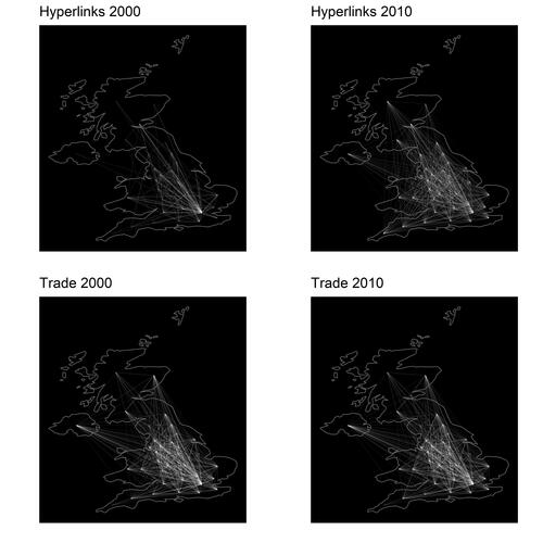
Furthermore, Figure 1 plots the interregional flows for both hyperlinks and trade for the first and the last year of our study period. In 2000, hyperlinks were primarily concentrated in the southeast of England. By 2010, however, we begin to see a similar pattern to the trade links, with the major flows still coming from the same regions, but with wider coverage. We can observe an increase in the flow intensity between 2000 and 2010, but this is higher for the hyperlinks. In total, we have data for 1,369 pairs between thirty-seven NUTS2 regions for eleven years (2000–2010).

Figure 1 Interregional trade and hyperlink flows.

Results

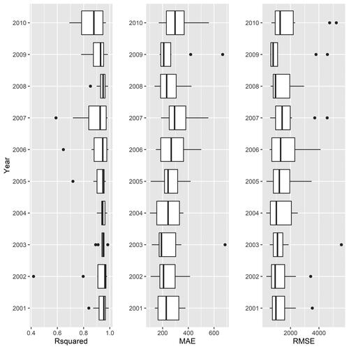
The first step of the analysis involves training our RF models using data from years t and t + 1. Figure 2 presents the accuracy metrics for the training data set that were obtained through the tenfold CV. The results clearly indicate that our models achieve high in-sample accuracy across all three prediction accuracy metrics employed here. There is some variation between years, but the results still appear to be very promising.

Figure 2 Accuracy metrics. Note: MAE = mean absolute error; RMSE = root mean square error.

To avoid overfitting and test the predictive capacity of our models on unseen data, the models estimated using data from years t and t + 1 are applied on years t + 2. In other words, we used the models trained with data from years t and t + 1 and the explanatory variables for year t + 2 to forecast interregional trade for year t + 2. The yearly accuracy metrics are presented in Table 3 and the predicted versus the observed flows of interregional trade are plotted in Figure 3. Indeed, our models are able to make highly accurate temporal out of sample predictions for interregional trade in the United Kingdom. The R² only drops below 0.9 in 2005 and 2010 (0.89 and 0.63), and it exceeds 0.95 in 2002 and 2004.⁶ The drop of the predictive capacity of our model for 2010 can be attributed to the aftermath of the financial crisis and the use of data reflecting different business cycles—before and after the crisis. As Figure 3 indicates, the highest errors are observed for the regional pairs with the two highest flows of interregional trade every year and our models under- and overestimate their flows. These outliers are always the intraregional flows within the inner and outer London regions (UKI1 and UKI2). With the exception of these extreme values, though (trade flows above $\pounds 50$ billion), our model performs remarkably well in temporal out of sample predictions.

Figure 3 Predicted versus observed interregional trade (in £100,000s) by year.

Table 3. Accuracy metrics for predicting unseen data from t + 2

Year	RMSE	R^2	MAE
2002	937.93	0.96	159.87
2003	1360.28	0.94	244.75
2004	1014.83	0.95	179.15
2005	1790.07	0.89	304.86
2006	1706.73	0.92	309.16
2007	1920.11	0.91	210.23
2008	1558.92	0.92	233.35
2009	1353.12	0.93	202.70
2010	3170.16	0.63	303.68

Note: RMSE = root mean square error; MAE = mean absolute error.

Articles attempting to estimate subnational or national trade flows from a national or supranational input–output tables by means of location quotients techniques normally present larger error terms. For example, Pereira-López, Carrascal-Incera, and Fernández-Fernández (2020), using a novel method, obtained errors for the domestic multipliers between 17.22 to 20.68, depending on the country studied. In a different study by Jiang, Dietzenbacher, and Los (2012), when estimating the input–output tables of Chinese regions, they obtained errors from 32.9 to 38.5 using traditional regionalization methods. These errors are measured as weighted absolute percentage errors (WAPEs; Sawyer and Miller 1983). WAPEs express the absolute deviation in relation to the true value of each input–output coefficient. In other words, they report average error in percentage terms (Lamonica and Chelli 2018; Pereira-López, Carrascal-Incera, and Fernández-Fernández 2020). In both cases these estimations were done for separate economies (single table), which means that they were estimating intraregional (or intracountry) sectoral trade flows (but bilateral sector flows in any case).

Our research framework enables us to disaggregate our results in terms of economic sectors. We therefore repeat the same modeling procedure for each sector separately and Figure 4 reports the R² values for the predictions of the unseen t + 2 interregional trade flows for each sector. In general, our models achieve higher accuracy in trade of goods (s1–s8) than services (s10–s15), which are conventionally considered as nontradable (Jensen et al. 2005). We can also observe a drop in accuracy for service sectors in 2010 due to the financial crisis and the related knock-on effects. The decrease of interregional trade volume makes it more difficult to predict. As expected, our model performs worse in some specific sectors. The most obvious example is hospitality (s11), for which the R² between the predicted and observed values for 2004 and 2010 drops below 0.25 and it does not exceed 0.75 for the whole study period. This can be attributed to the strong local and intraregional trade dependencies of this sector. A similar trend—although not as dramatic—can be observed for real estate.

Figure 4 R² for t + 2 out-of-sample predictions per sector. Note: s1 = agriculture; s2 = mining; s3 = food; s4 = textiles; s5 = chemicals; s6 = equipment; s8 = manufacturing; s9 = construction; s10 = distribution; s11 = hospitality; s12 = transport; s13 = financial; s14 = real estate; s15 = nonmarket services.

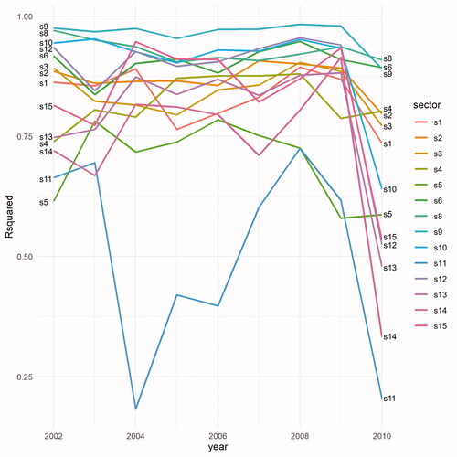
With the exception of 2010, the predictive capacity of our models is high for all the sectors, as R² is consistently above 0.75. Our models perform exceptionally well in predicting unseen interregional trade flows regarding manufacturing and construction as well as equipment.

In summary, our results show a clear pattern of tradable sectors versus nontradable sectors. Even though references such as Gervais and Jensen (2019) and Jensen et al. (2005) challenge this conventional view of goods as tradable and services as nontradable, Gervais and Jensen (2019), for the United States they found that manufacturing products are 75 percent tradable and 25 percent nontradable (S3–S8 sectors in our study), recreation and food services (the most comparable to our hospitality sector) is 86 percent nontradable, and real estate and leasing is 79 percent nontradable, among other results they obtained.

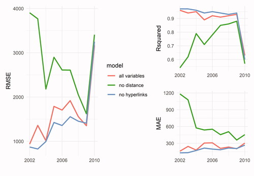
To further assess the role of our main variable of interest—the volume of hyperlinks between regions—in predicting interregional trade flows, we estimate the first set of models for the total trade flows using alternative specifications by excluding (1) the distance, and (2) the hyperlinks features. The accuracy metrics for the out-of-sample predictions for unseen trade flow data from years t + 2 are presented in Figure 5, which also includes the metrics for the base models presented in Table 3 for direct comparison. The main message from Figure 5 is that distance plays the most important role in predicting interregional trade flows. All three metrics are worst when the distance is excluded. This is not surprising, as the role of distance in predicting trade and other types of spatial interactions has been extensively highlighted in the literature discussed earlier. There are two key messages from Figure 5. First, achieving R² values of up to 0.86 without using a physical distance feature, which has traditionally been the main explanatory variable of bilateral trade, is indicative of the predictive power of our hyperlinks approach. Second, the gap in terms of the prediction accuracy between the models with and without distance decreases over time. This illustrates that over time, as the adoption rate of Web technologies increased, interregional trade flows left more “digital breadcrumbs” behind, and, therefore, are better reflected in the volumes of interregional hyperlinks (Rabari and Storper 2015). Nevertheless, the predictive capacity of distance remains unchallenged at large, as the green lines in Figure 5 indicate.

Figure 5 Accuracy metrics for alternative specifications. Note: MAE = mean absolute error; RMSE = root mean square error.

To further assess the robustness of our results, we repeat our workflow for a different sample of Web sites. Instead of including only the Web sites with a unique postcode, we add in our sample Web sites with up to ten unique postcodes. As discussed earlier, this enhanced sample of Web sites containing multiple postcodes within the Web text represents commercial Web sites with multiple locations. Given that we are not able to distinguish the role of these different locations, we expect that using this sample for training and testing our models will lead to more noise. Nevertheless, the predictive capacity of our models remains almost unchanged according to the out-of-sample prediction metrics, which are reported in Table 4, and the predicted versus the observed interregional trade flows, which are plotted in Figure 6. Indeed, R² drops below 0.90 for only two years (2009 and 2010). Again, the largest prediction errors are linked to the regional pairs with the highest volume of regional trade—that is London’s intraregional trade.

Figure 6 Predicted versus observed interregional trade (in £100,000s) by year for Web sites with multiple postcodes.

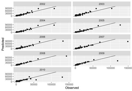
Table 4. Accuracy metrics in unseen data with multiple postcodes from t + 2

Year	RMSE	R^2	MAE
2002	1181.91	0.94	244.27
2003	1428.99	0.93	282.77
2004	1011.14	0.95	173.31
2005	1414.77	0.94	232.25
2006	1433.92	0.94	208.32
2007	1894.59	0.91	227.77
2008	1206.3	0.95	249.66
2009	2008.83	0.81	238.38
2010	2500.1	0.78	298.27

Note: RMSE = root mean square error; MAE = mean absolute error.

A Local-Level Application

The final step in our workflow is to use the NUTS2 models we trained and validated for a more spatially disaggregated application. This exercise illustrates the value of our research framework in mapping interregional trade flows at a disaggregated spatial level, at which such data are not usually collected. Specifically, we take advantage of the point nature of our hyperlink data and we aggregate them at the local authority district (LAD) level. This is the main subnational administrative division in the United Kingdom. We then apply the NUTS2 model, which was trained on data from 2008 and 2009 and tested on 2010 trade data, to the LAD hyperlinks, employment, population density, and distance data, and we make predictions regarding LAD-to-LAD trade flows for 2010, the most recent data.⁷ Although we are not able to validate these predictions at the LAD level, as there are no trade data available at this level, this exercise provides a unique opportunity to map trade flows at this level of spatial granularity.

We briefly discuss here the predictions for two LADs: Camden in central London and Birmingham, the second biggest city in the United Kingdom. We present the import and export trade flows for these LADs in Figure 7.⁸ Although both of these examples illustrate the importance of distance in trade flows—light-colored lines are concentrated near Camden and Birmingham—Camden appears to have more light-colored links not only with adjacent LADs, but also with more distant ones both in terms of imports and exports. Not surprisingly, Camden’s reach appears to be more extended than that of Birmingham.

Figure 7 Local authority districts’ trade flow predictions (in £100,000s): Birmingham exports (top left), Birmingham imports (top right), Camden exports (bottom left), –and Camden imports (bottom right).

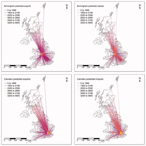
The preceding example illustrates the capacity of our research framework for spatially disaggregated analysis of trade flows. To our knowledge, observed trade data at this level are very hard to find. Importantly, though, the LAD level in the United Kingdom represents administrative units and, therefore, our framework can be used by local authorities to design relevant local policies. Without these data and a modeling framework at this geographical level, it is nearly impossible to do accurate ex ante evaluations of place-based policies. With these predictions, any LAD could calculate the net impact of a policy in their region and estimate the possible benefits for the residents.

Conclusions

Despite the complexity of interregional trade and its importance in regional economic performance and, consequently, regional economic policies, it is well established in the literature that interregional trade is difficult to observe. This is because such data are mostly available at a country level and hardly ever are monitored at a local or regional level. The current state of the art of empirical studies focusing on modeling international trade tend to be explanatory in their nature and are mostly based on pure distance decay measures.

Our article aims to address this gap by proposing an innovative research framework, which is based on openly accessible Web data and predictive models. On top of using variables such as distance, employment, and population density, we employ Web data regarding the number of hyperlinks between geolocated commercial Web sites aggregated at the regional level during the period between 2000 and 2010. These data, in essence, represent the digital breadcrumbs that trade leaves behind nowadays, and we use them to predict interregional trade flows. By building a rolling forecasting workflow based on RF we are able to achieve very accurate out-of-sample temporal predictions of interregional trade flows in the United Kingdom. We are able to also disaggregate our models at a sectoral level and illustrate the sectors for which our models perform better. This sectoral variation in our predictive capacity matches our expectations, which are rooted in the relevant literature. We also perform different sensitivity tests, which further reinforce the value of our framework. Finally, we use our regional models to produced spatially disaggregated trade flows at a local level—the UK LAD. This is of particular importance, as this is the main subnational administrative authority in the United Kingdom and such illustrations can be helpful to design local economic policies.

The current wide availability of archived data makes our framework easily applicable to different temporal and geographical contexts. Hence, using more recent archived Web data, something that involves up-front investment regarding developing the necessary software infrastructure, will allow the now-casting of interregional trade data for a variety of local scales to many administrative authorities responsible for designing local and regional economic policies. Identifying these types of external dependencies and vulnerabilities to supply chain disruptions is essential for regional well-being, as the recent COVID-19 crisis has shown us. This can help us to anticipate local exposures and knock-on effects to shocks and to elaborate mitigating policies almost in real time.

Acknowledgments

The authors would like to thank the editor and the anonymous reviewers for their constructive comments. The first author would also like to thank the QuSS Research Group at the School of Geographical Sciences at the University of Bristol and also the participants and the organizers of the Spatial Analytics + Data seminar series.

Additional information

Notes on contributors

Emmanouil Tranos

EMMANOUIL TRANOS is a Professor of Quantitative Human Geography, University of Bristol, Bristol BS8 1SS, UK, and a fellow in the Alan Turing Institute. E-mail: [email protected]. His research has been exposing the spatial dimensions of digital technologies and the digital economy from their early stages until today.

André Carrascal-Incera

ANDRÉ CARRASCAL-INCERA is an Assistant Professor in the Department of Economics, University of Oviedo, Asturias 33006, Spain. E-mail: [email protected]. His lines of research are related to the generation and distribution of income in multiregional systems and the development of economy-wide models at the regional level.

George Willis

GEORGE WILLIS is a Doctoral Student in the School of Geography, University of Birmingham, Birmingham B15 2TT, UK. E-mail: [email protected]. His research interests include quantitative methods in geography, focusing on the spatiotemporal patterns of urban shrinkage in China.

Notes

1 In this article we use the terms regional and subnational interchangeably.

2 See also the randomForest R package, which is based on Breiman’s (2001) original implementation.

3 See https://data.webarchive.org.uk/opendata/ukwa.ds.2/.

4 See https://archive.org/.

5 For example, the Web pages http://www.examplewebsite.co.uk/webpage1 and http://www.examplewebsite.co.uk/webpage2 are part of the http://www.examplewebsite.co.uk/website.

6 As a comparison, the Appendix provides the same results based on a LASSO estimator, which are inferior to the ones acquired through RF.

7 We opted to present the predictions for 2010, as this was the latest year for which we had data.

8 The Appendix provides the URL to interactive visualizations of the hyperlink flows at the NUTS2 level and the trade flow predictions for LADs.

Appendix

Online material

An interactive map of the hyperlink data and thetrade flow predictions between Local Authority Districts can be found at https://etranos.info/regional_trade_hyperlinks/.

Out of sample R² for different sectors

 

Lasso regressions

 

Data wrangling process

This section describes how geographic regions were added to the host-linkage dataset provided by JISC UK Web Domain Dataset (Jackson 2017a). The archived web data are from 2000-2010. The process begins combining the host-host links to a file containing unique postcodes for each host ending in co.uk. An example is provided below in Tables A.3. and A.4.

The two data frames were joined by matching the variable domain. If an origin or destination was found in in the postcode data, it was added to the file. Host-links without a postcode were dropped. This leaves with host, domain and postcode for origins and destinations and the number of links between. This is shown below in Table A.5.

The next step was to remove websites that linked to themselves (e.g., the first row above). These data were not of interest as we are looking for links between different websites. Therefore, if origin host and destination host were the same, they were dropped. We now have host-to-host links with the associated unique postcodes and the number of links.

The next step was to aggregate to the NUTS2 regions (Table A.6.). This was done by using a postcode to NUTS2 (2010 version) lookup file combined with the above created data. The data was then aggregated summing all data with the same origin NUTS and destination NUTS codes. We are then left with our NUTS2-to-NUTS2 links.

The same process was done for every year 2000-2010.

Table A.1. R-squared for t + 2 out of sample predictions per sector

Sector	2002	2003	2004	2005	2006	2007	2008	2009	2010
s1	0.863	0.855	0.890	0.764	0.798	0.832	0.894	0.869	0.735
s2	0.885	0.861	0.864	0.866	0.856	0.907	0.901	0.892	0.797
s3	0.892	0.823	0.815	0.795	0.846	0.857	0.904	0.885	0.772
s4	0.739	0.805	0.790	0.871	0.876	0.876	0.880	0.788	0.802
s5	0.615	0.782	0.717	0.738	0.784	0.752	0.725	0.580	0.587
s6	0.917	0.837	0.902	0.911	0.882	0.926	0.947	0.910	0.893
s8	0.970	0.951	0.936	0.905	0.914	0.907	0.921	0.936	0.909
s9	0.976	0.968	0.974	0.954	0.972	0.973	0.983	0.980	0.890
s10	0.944	0.953	0.926	0.903	0.930	0.927	0.951	0.934	0.640
s11	0.664	0.695	0.183	0.420	0.398	0.602	0.725	0.618	0.204
s12	0.935	0.845	0.926	0.896	0.905	0.932	0.955	0.940	0.524
s13	0.748	0.764	0.874	0.838	0.869	0.835	0.877	0.882	0.478
s14	0.721	0.668	0.817	0.811	0.795	0.711	0.805	0.914	0.332
s15	0.815	0.773	0.947	0.911	0.910	0.822	0.870	0.934	0.534

s1: Agriculture, s2: Mining, s3: Food, s4: Textiles, s5: Chemicals, s6: Equipment, s8: Manufacturing; s9: Construction, s10: Distribution, s11: Hospitality, s12: Transport, s13: Financial, s14: Real Estate, s15: Non-Market Services.

Table A.2. LASSO regressions: Accuracy metrics in unseen data from t + 2

Year	RMSE	R^2	MAE
2002	3416.15	0.64	1233.66
2003	16642.84	0.24	2172.69
2004	2887.28	0.64	1090.96
2005	4441.22	0.43	1006.57
2006	4418.99	0.36	1153.61
2007	4781.95	0.38	1222.12
2008	6178.04	0.26	1262.79
2009	3918.96	0.42	1259.55
2010	4445.62	0.3	1150.39

Note: RMSE = root mean square error; MAE = mean absolute error.

Table A.3. Host-linkage file

Year	Origin	Destination	Links
2000	btclickbus.excite.co.uk	greenwich2000.co.uk	1
2000	btclickfree.excite.co.uk	www.rockvillecenter.com	2
2000	adapthorpe.com	www.adapthorpe.com	1
2000	btclickfam.excite.co.uk	conciergedesk.co.uk	1
2000	formby.wiganmbc.gov.uk	www.charitynet.org	1

Table A.4. Websites with unique postcodes

URL	Postcode	Year	Host	Domain
20000609075945/http://altberg.co.uk:80/military_boots.htm	DL10 4XB	2000	altberg.co.uk	altberg
20001003045622/http://www.guest-house.demon.co.uk:80/	CB2 1AA	2000	www.guest-house.demon.co.uk	demon
20000917204128/http://www.millenniumit.co.uk:80/CV.htm	E3 5AN	2000	www.millenniumit.co.uk	millenniumit
20000312143711/http://www.nova-tech.co.uk:80/page2.html	PR9 9DZ	2000	www.nova-tech.co.uk	nova-tech
20000914061255/http://www.aleontap.co.uk:80/weblinks/	WR6 6DH	2000	www.aleontap.co.uk	aleontap

Table A.5. Combined host and postcode data

Origin.host	Orig.domain	Origin.pc	Dest.host	Dest.domain	Ddest.pc	Links
24carat.co.uk	24carat	FY4 1RJ	24carat.co.uk	24carat	FY4 1RJ	9201
www.lifestyle.co.uk	lifestyle	WC1A 2AE	www.lupine.demon.co.uk	demon	KT17 2HB	3
www.barcodes.beechman- online.co.uk	beechman- online	BR1 1PD	www.ao.beechman-online.co.uk	beechman- online	BR1 1PD	3
www.bringfrd.demon.co.uk	demon	NN6 6HB	www.bringfrd.demon.co.uk	demon	NN6 6HB	28

Table A.6. NUTS2 level data

Origin	Destination	Weight UKC1
UKC1	90
UKC1	UKC2	1
UKC1	UKE2	1
UKC1	UKH3	1
UKC1	UKI1	3

References

- Ainsworth, S. G., A. Alsum, H. SalahEldeen, M. C. Weigle, and M. L. Nelson. 2011. How much of the web is archived? In Proceedings of the 11th annual International ACM/IEEE Joint Conference on Digital Libraries, 133–36. New York: ACM.
- Anderson, J. E., and E. Van Wincoop. 2003. Gravity with gravitas: A solution to the border puzzle. American Economic Review 93 (1):170–92. doi: 10.1257/000282803321455214.
- Antras, P., and D. Chor. 2018. On the measurement of upstreamness and downstreamness in global value chains. Technical report, National Bureau of Economic Research, Cambridge, MA.
- Arto, I., J. M. Rueda-Cantuche, and G. P. Peters. 2014. Comparing the GTAP-MRIO and WIOD databases for carbon footprint analysis. Economic Systems Research 26 (3):327–53. doi: 10.1080/09535314.2014.939949.
- Athey, S., and G. W. Imbens. 2019. Machine learning methods that economists should know about. Annual Review of Economics 11 (1):685–725. doi: 10.1146/annurev-economics-080217-053433.
- Barca, F. 2009. An agenda for a reformed cohesion policy-independent report. Brussels, Belgium: European Commission.
- Biau, G. 2012. Analysis of a random forests model. Journal of Machine Learning Research 13:1063–95.
- Blazquez, D., and J. Domenech. 2018. Big data sources and methods for social and economic analyses. Technological Forecasting and Social Change 130:99–113. doi: 10.1016/j.techfore.2017.07.027.
- Boero, R., B. K. Edwards, and M. K. Rivera. 2018. Regional input–output tables and trade flows: An integrated and interregional non-survey approach. Regional Studies 52 (2):225–38. doi: 10.1080/00343404.2017.1286009.
- Breiman, L. 2001. Random forests. Machine Learning 45 (1):5–32. doi: 10.1023/A:1010933404324.
- Caruana, R., N. Karampatziakis, and A. Yessenalina. 2008. An empirical evaluation of supervised learning in high dimensions. In Proceedings of the 25th International Conference on Machine Learning, ICML ’08, 96–103. New York: Association for Computing Machinery. doi: 10.1145/1390156.1390169.
- Chen, W., B. Los, P. McCann, R. Ortega-Argilés, M. Thissen, and F. van Oort. 2018. The continental divide? Economic exposure to Brexit in regions and countries on both sides of The Channel. Papers in Regional Science 97 (1):25–54. doi: 10.1111/pirs.12334.
- Chun, Y., H. Kim, and C. Kim. 2012. Modeling interregional commodity flows with incorporating network autocorrelation in spatial interaction models: An application of the US interstate commodity flows. Computers, Environment and Urban Systems 36 (6):583–91. doi: 10.1016/j.compenvurbsys.2012.04.002.
- Chung, J. 2011. The geography of global Internet hyperlink networks and cultural content analysis. PhD dissertation, University at Buffalo.
- Crampton, J. W., M. Graham, A. Poorthuis, T. Shelton, M. Stephens, M. W. Wilson, and M. Zook. 2013. Beyond the geotag: Situating “big data” and leveraging the potential of the geoweb. Cartography and Geographic Information Science 40 (2):130–39. doi: 10.1080/15230406.2013.777137.
- Credit, K. 2022. Spatial models or random forest? Evaluating the use of spatially explicit machine learning methods to predict employment density around new transit stations in Los Angeles. Geographical Analysis 54 (1):58–83. doi: 10.1111/gean.12273.
- David, H., D. Dorn, and G. H. Hanson. 2013. The China syndrome: Local labor market effects of import competition in the United States. American Economic Review 103 (6):2121–68. doi: 10.1257/aer.103.6.2121.
- de Mello-Sampayo, F. 2017a. Competing-destinations gravity model applied to trade in intermediate goods. Applied Economics Letters 24 (19):1378–84. doi: 10.1080/13504851.2017.1282109.
- de Mello-Sampayo, F. 2017b. Testing competing destinations gravity models—Evidence from BRIC International. The Journal of International Trade & Economic Development 26 (3):277–94. doi: 10.1080/09638199.2016.1239752.
- Devriendt, L., B. Derudder, and F. Witlox. 2008. Cyberplace and cyberspace: Two approaches to analyzing digital intercity linkages. Journal of Urban Technology 15 (2):5–32. doi: 10.1080/10630730802401926.
- Dietzenbacher, E., B. Los, R. Stehrer, M. Timmer, and G. De Vries. 2013. The construction of world input–output tables in the WIOD project. Economic Systems Research 25 (1):71–98. doi: 10.1080/09535314.2012.761180.
- Egger, P. 2002. An econometric view on the estimation of gravity models and the calculation of trade potentials. The World Economy 25 (2):297–312. doi: 10.1111/1467-9701.00432.
- Feenstra, R. C., R. E. Lipsey, H. Deng, A. C. Ma, and H. Mo. 2005. World trade flows: 1962–2000. Technical report, National Bureau of Economic Research, Cambridge, MA.
- Fingleton, B., H. Garretsen, and R. Martin. 2012. Recessionary shocks and regional employment: Evidence on the resilience of UK regions. Journal of Regional Science 52 (1):109–33. doi: 10.1111/j.1467-9787.2011.00755.x.
- Flegg, A. T., and C. D. Webber. 2000. Regional size, regional specialization and the FLQ formula. Regional Studies 34 (6):563–69. doi: 10.1080/00343400050085675.
- Gervais, A., and J. B. Jensen. 2019. The tradability of services: Geographic concentration and trade costs. Journal of International Economics 118:331–50. doi: 10.1016/j.jinteco.2019.03.003.
- Gómez-Herrera, E. 2013. Comparing alternative methods to estimate gravity models of bilateral trade. Empirical Economics 44 (3):1087–1111. doi: 10.1007/s00181-012-0576-2.
- Greene, W. 2013. Export potential for US advanced technology goods to India using a gravity model approach. Working Paper 2013-03B, U.S. International Trade Commission, Washington, DC.
- Guan, D., D. Wang, S. Hallegatte, S. J. Davis, J. Huo, S. Li, Y. Bai, T. Lei, Q. Xue, D. Coffman, et al. 2020. Global supply-chain effects of COVID-19 control measures. Nature Human Behaviour 4 (6):577–87. doi: 10.1038/s41562-020-0896-8.
- Guns, R., and R. Rousseau. 2014. Recommending research collaborations using link prediction and random forest classifiers. Scientometrics 101 (2):1461–73. doi: 10.1007/s11192-013-1228-9.
- Halavais, A. 2000. National borders on the world wide web. New Media & Society 2 (1):7–28. doi: 10.1177/14614440022225689.
- Hale, S. A., T. Yasseri, J. Cowls, E. T. Meyer, R. Schroeder, and H. Margetts. 2014. Mapping the UK webspace: Fifteen years of British universities on the web. In Proceedings of the 2014 ACM Conference on Web Science, 62–70. New York: ACM.
- Head, K., T. Mayer, and J. Ries. 2009. How remote is the offshoring threat? European Economic Review 53 (4):429–44. doi: 10.1016/j.euroecorev.2008.08.001.
- Hellmanzik, C., and M. Schmitz. 2015. Gravity and international services trade: The impact of virtual proximity. European Economic Review 77:82–101. doi: 10.1016/j.euroecorev.2015.03.014.
- Hellmanzik, C., and M. Schmitz. 2017. Taking gravity online: The role of virtual proximity in international finance. Journal of International Money and Finance 77:164–79. doi: 10.1016/j.jimonfin.2017.07.001.
- Hernández, B., J. Jiménez, and M. J. Martín. 2009. Improved estimation of regional input–output tables using cross-regional methods. International Journal of Information Management 29 (5):362–71. doi: 10.1016/j.ijinfomgt.2008.12.006.
- Holmberg, K. 2010. Co-inlinking to a municipal Web space: A webometric and content analysis. Scientometrics 83 (3):851–62. doi: 10.1007/s11192-009-0148-1.
- Holmberg, K., and M. Thelwall. 2009. Local government web sites in Finland: A geographic and webometric analysis. Scientometrics 79 (1):157–69. doi: 10.1007/s11192-009-0410-6.
- Holzmann, H., W. Nejdl, and A. Anand. 2016. The dawn of today’s popular domains: A study of the archived German Web over 18 years. In Digital Libraries (JCDL), 2016 IEEE/ACM Joint Conference, 73–82. IEEE.
- Hope, O. 2017. The changing face of the online world. Accessed March 5, 2021. https://www.nominet.uk/changing-face-online-world/.
- Ijtsma, P., and B. Los. 2020. UK Regions in global value chains. Technical report, Economic Statistics Centre of Excellence (ESCoE), London.
- Isard, W. 1951. Interregional and regional input–output analysis: A model of a space-economy. The Review of Economics and Statistics 33 (4):318–28. doi: 10.2307/1926459.
- Isard, W. 1956. Location and space-economy. New York: The Technology Press of Massachusetts Institute of Technology and John Wiley & Sons, Inc.
- Ivanova, O., D. Kancs, and M. Thissen. 2019. Regional trade flows and input output data for Europe. Technical report, EERI Research Paper Series, Brussels, Belgium.
- Jackson, A. N. 2017a. JISC UK Web domain dataset (1996–2010) Geoindex. https://doi.org/10.5259/ukwa.ds.2/geo/1
- Jackson, A. N. 2017b. JISC UK Web domain dataset (1996–2010) Host Link Graph. https://doi.org/10.5259/ukwa.ds.2/host.linkage/1
- Janc, K. 2015a. Geography of hyperlinks–Spatial dimensions of local government websites. European Planning Studies 23 (5):1019–37. doi: 10.1080/09654313.2014.889090.
- Janc, K. 2015b. Visibility and connections among cities in digital space. Journal of Urban Technology 22 (4):3–21. doi: 10.1080/10630732.2015.1073899.
- Jensen, J. B., L. G. Kletzer, J. Bernstein, and R. C. Feenstra. 2005. Tradable services: Understanding the scope and impact of services offshoring [with comments and discussion]. Brookings Trade Forum 2005 (1):75–133. doi: http://www.jstor.org/stable/25058763.
- Jiang, X., E. Dietzenbacher, and B. Los. 2012. Improved estimation of regional input–output tables using cross-regional methods. Regional Studies 46 (5):621–37. doi: 10.1080/00343404.2010.522566.
- JISC and the Internet Archive. 2013. JISC UK Web domain dataset (1996–2013). The British Library. https://doi.org/10.5259/ukwa.ds.2/1
- Jones, B. W., B. Spigel, and E. J. Malecki. 2010. Blog links as pipelines to buzz elsewhere: The case of New York theater blogs. Environment and Planning B: Planning and Design 37 (1):99–111. doi: 10.1068/b35026.
- Keßler, C. 2017. Extracting central places from the link structure in Wikipedia. Transactions in GIS 21 (3):488–502. doi: 10.1111/tgis.12284.
- Kimura, F., and H.-H. Lee. 2006. The gravity equation in international trade in services. Review of World Economics 142 (1):92–121. doi: 10.1007/s10290-006-0058-8.
- Kitsos, A., A. Carrascal-Incera, and R. Ortega-Argilés. 2019. The role of embeddedness on regional economic resilience: Evidence from the UK. Sustainability 11 (14):3800. doi: 10.3390/su11143800.
- Kleinberg, J., J. Ludwig, S. Mullainathan, and Z. Obermeyer. 2015. Prediction policy problems. The American Economic Review 105 (5):491–95. doi: 10.1257/aer.p20151023.
- Krüger, M., J. Kinne, D. Lenz, and B. Resch. 2020. The digital layer: How innovative firms relate on the web. Discussion Paper 20-003, ZEW-Centre for European Economic Research. Leibniz-Zentrum für Europäische Wirtschaftsforschung, Mannheim.
- Kuhn, M. 2008. Building predictive models in R using the caret package. Journal of Statistical Software 28 (5):1–26. doi: 10.18637/jss.v028.i05.
- Lamonica, G. R., and F. M. Chelli. 2018. The performance of non-survey techniques for constructing sub-territorial input-output tables. Papers in Regional Science 97 (4):1169–1202. doi: 10.1111/pirs.12297.
- Last, M., O. Maimon, and E. Minkov. 2002. Improving stability of decision trees. International Journal of Pattern Recognition and Artificial Intelligence 16 (2):145–59. doi: 10.1142/S0218001402001599.
- Lazer, D., A. Pentland, L. Adamic, S. Aral, A.-L. Barabasi, D. Brewer, N. Christakis, N. Contractor, J. Fowler, M. Gutmann, et al. 2009. Social science: Computational social science. Science 323 (5915):721–23. doi: 10.1126/science.1167742.
- Leamer, E., and R. Stern. 1971. Quantitative international economics. Journal of International Economics 1:359–61.
- Liaw, A., and M. Wiener. 2002. Classification and regression by randomForest. R News 2 (3):18–22.
- Lin, J., A. Halavais, and B. Zhang. 2007. The blog network in America: Blogs as indicators of relationships among US cities. Connections 27 (2):15–23.
- Linnemann, H. 1966. An econometric study of international trade flows. Amsterdam, The Netherlands: Holland Publishing.
- Los, B., P. McCann, J. Springford, and M. Thissen. 2017. The mismatch between local voting and the local economic consequences of Brexit. Regional Studies 51 (5):786–99. doi: 10.1080/00343404.2017.1287350.
- Los, B., M. P. Timmer, and G. J. de Vries. 2015. How global are global value chains? A new approach to measure international fragmentation. Journal of Regional Science 55 (1):66–92. doi: 10.1111/jors.12121.
- Los, B., M. P. Timmer, and G. J. de Vries. 2016. Tracing value-added and double counting in gross exports: Comment. American Economic Review 106 (7):1958–66. doi: 10.1257/aer.20140883.
- Matter, R. 2009. Economic recovery: Innovation and sustainable growth. Paris: OECD.
- McCann, P., and R. Ortega-Argilés. 2015. Smart specialization, regional growth and applications to European Union cohesion policy. Regional Studies 49 (8):1291–1302. doi: 10.1080/00343404.2013.799769.
- Meijers, E., and A. Peris. 2019. Using toponym co-occurrences to measure relationships between places: Review, application and evaluation. International Journal of Urban Sciences 23 (2):246–68. doi: 10.1080/12265934.2018.1497526.
- Mikkonen, K., and M. Luoma. 1999. The parameters of the gravity model are changing—How and why? Journal of Transport Geography 7 (4):277–83. doi: 10.1016/S0966-6923(99)00024-1.
- Miller, R. E., and P. D. Blair. 2009. Input–output analysis: Foundations and extensions. New York: Cambridge University Press.
- Mozolin, M., J.-C. Thill, and E. Lynn Usery. 2000. Trip distribution forecasting with multilayer perceptron neural networks: A critical evaluation. Transportation Research Part B: Methodological 34 (1):53–73. doi: 10.1016/S0191-2615(99)00014-4.
- Mullainathan, S., and J. Spiess. 2017. Machine learning: An applied econometric approach. Journal of Economic Perspectives 31 (2):87–106. doi: 10.1257/jep.31.2.87.
- Musso, M., and F. Merletti. 2016. This is the future: A reconstruction of the UK business web space (1996–2001). New Media & Society 18 (7):1120–42. doi: 10.1177/1461444816643791.
- Ortega, J. L., and I. F. Aguillo. 2008a. Linking patterns in European Union countries: Geographical maps of the European academic web space. Journal of Information Science 34 (5):705–14. doi: 10.1177/0165551507086990.
- Ortega, J. L., and I. F. Aguillo. 2008b. Visualization of the Nordic academic web: Link analysis using social network tools. Information Processing & Management 44 (4):1624–33. doi: 10.1016/j.ipm.2007.09.010.
- Ortega, J. L., and I. F. Aguillo. 2009. Mapping world-class universities on the web. Information Processing & Management 45 (2):272–79. doi: 10.1016/j.ipm.2008.10.001.
- Oshan, T. M. 2020a. Potential and pitfalls of big transport data for spatial interaction models of urban mobility. The Professional Geographer 72 (4):468–80. doi: 10.1080/00330124.2020.1787180.
- Oshan, T. M. 2020b. The spatial structure debate in spatial interaction modeling: 50 years on. Progress in Human Geography 45 (5):925–50.
- Owen, A., R. Wood, J. Barrett, and A. Evans. 2016. Explaining value chain differences in MRIO databases through structural path decomposition. Economic Systems Research 28 (2):243–72. doi: 10.1080/09535314.2015.1135309.
- Paul Lesage, J., and W. Polasek. 2008. Incorporating transportation network structure in spatial econometric models of commodity flows. Spatial Economic Analysis 3 (2):225–45. doi: 10.1080/17421770801996672.
- Pereira-López, X., A. Carrascal-Incera, and M. Fernández-Fernández. 2020. A bidimensional reformulation of location quotients for generating input–output tables. Spatial Economic Analysis 15 (4):476–93. doi: 10.1080/17421772.2020.1729996.
- Pontius, R. G., O. Thontteh, and H. Chen. 2008. Components of information for multiple resolution comparison between maps that share a real variable. Environmental and Ecological Statistics 15 (2):111–42. doi: 10.1007/s10651-007-0043-y.
- Pourebrahim, N., S. Sultana, A. Niakanlahiji, and J.-C. Thill. 2019. Trip distribution modeling with Twitter data. Computers, Environment and Urban Systems 77:101354. doi: 10.1016/j.compenvurbsys.2019.101354.
- Rabari, C., and M. Storper. 2015. The digital skin of cities: Urban theory and research in the age of the sensored and metered city, ubiquitous computing and big data. Cambridge Journal of Regions, Economy and Society 8 (1):27–42. doi: 10.1093/cjres/rsu021.
- Ren, Y., T. Xia, Y. Li, and X. Chen. 2019. Predicting socio-economic levels of urban regions via offline and online indicators. PLoS ONE 14 (7):e0219058. doi: 10.1371/journal.pone.0219058.
- Riddington, G., H. Gibson, and J. Anderson. 2006. Comparison of gravity model, survey and location quotient-based local area tables and multipliers. Regional Studies 40 (9):1069–81. doi: 10.1080/00343400601047374.
- Salvini, M. M., and S. I. Fabrikant. 2016. Spatialization of user-generated content to uncover the multirelational world city network. Environment and Planning B: Planning and Design 43 (1):228–48. doi: 10.1177/0265813515603868.
- Sargento, A. L., P. N. Ramos, and G. J. Hewings. 2012. Inter-regional trade flow estimation through non-survey models: An empirical assessment. Economic Systems Research 24 (2):173–93. doi: 10.1080/09535314.2011.574609.
- Sawyer, C. H., and R. E. Miller. 1983. Experiments in regionalization of a national input–output table. Environment and Planning A: Economy and Space 15 (11):1501–20. doi: 10.1068/a151501.
- Serrano, M. Á, and M. Boguñá. 2003. Topology of the world trade web. Physical Review E: Statistical, Nonlinear, and Soft Matter Physics 68 (1, Pt. 2):015101. doi: 10.1103/PhysRevE.68.015101.
- Simini, F., M. C. González, A. Maritan, and A.-L. Barabási. 2012. A universal model for mobility and migration patterns. Nature 484 (7392):96–100. doi: 10.1038/nature10856.
- Singleton, A., and D. Arribas-Bel. 2021. Geographic data science. Geographical Analysis 53 (1):61–75. doi: 10.1111/gean.12194.
- Sinha, P., A. E. Gaughan, F. R. Stevens, J. J. Nieves, A. Sorichetta, and A. J. Tatem. 2019. Assessing the spatial sensitivity of a random forest model: Application in gridded population modeling. Computers, Environment and Urban Systems 75:132–45. doi: 10.1016/j.compenvurbsys.2019.01.006.
- Sulaiman, S., S. Mariyam Shamsuddin, A. Abraham, and S. Sulaiman. 2011. Intelligent web caching using machine learning methods. Neural Network World 21 (5):429–52. doi: 10.14311/NNW.2011.21.025.
- Thelwall, M. 2000. Who is using the .co.uk domain? Professional and media adoption of the web. International Journal of Information Management 20 (6):441–53. https://www.sciencedirect.com/science/article/pii/S0268401200000384. doi: 10.1016/S0268-4012(00)00038-4.
- Thelwall, M. 2002a. Evidence for the existence of geographic trends in university web site interlinking. Journal of Documentation 58 (5):563–74. doi: 10.1108/00220410210441586.
- Thelwall, M. 2002b. The top 100 linked-to pages on UK university web sites: High inlink counts are not usually associated with quality scholarly content. Journal of Information Science 28 (6):483–91. doi: 10.1177/016555150202800604.
- Thelwall, M., and L. Vaughan. 2004. A fair history of the Web? Examining country balance in the Internet Archive. Library & Information Science Research 26 (2):162–76. doi: 10.1016/j.lisr.2003.12.009.
- Thelwall, M., L. Vaughan, and L. Björneborn. 2006. Webometrics. Annual Review of Information Science and Technology 39 (1):81–135. doi: 10.1002/aris.1440390110.
- Thissen, M., T. de Graaff, and F. van Oort. 2016. Competitive network positions in trade and structural economic growth: A geographically weighted regression analysis for European regions. Papers in Regional Science 95 (1):159–80. doi: 10.1111/pirs.12224.
- Thissen, M., D. Diodato, and F. Van Oort. 2013a. European regional trade flows: An update for 2000–2010. The Hague: PBL Netherlands Environmental Assessment Agency.
- Thissen, M., D. Diodato, and F. Van Oort. 2013b. Integrated regional Europe: European regional trade flows in 2000. The Hague: PBL Netherlands Environmental Assessment Agency.
- Thissen, M., M. Lankhuizen, F. van Oort, B. Los, and D. Diodato. 2018. EUREGIO: The construction of a global IO database with regional detail for Europe for 2000–2010. Tinbergen Institute Discussion Papers 18-084/VI, Tinbergen Institute.
- Timmer, M. P., E. Dietzenbacher, B. Los, R. Stehrer, and G. J. De Vries. 2015. An illustrated user guide to the world input–output database: The case of global automotive production. Review of International Economics 23 (3):575–605. doi: 10.1111/roie.12178.
- Tinbergen, J. 1962. Shaping the world economy. New York: The Twentieth Century Fund.
- Többen, J., and T. H. Kronenberg. 2015. Construction of multi-regional input–output tables using the CHARM method. Economic Systems Research 27 (4):487–507. doi: 10.1080/09535314.2015.1091765.
- Tranos, E., T. Kitsos, and R. Ortega-Argilés. 2021. Digital economy in the UK: Regional productivity effects of early adoption. Regional Studies 55 (12):1924–38. doi: 10.1080/00343404.2020.1826420.
- Tranos, E., and C. Stich. 2020. Individual internet usage and the availability of online content of local interest: A multilevel approach. Computers, Environment and Urban Systems 79:101371. doi: 10.1016/j.compenvurbsys.2019.101371.
- Vaughan, L. 2004. Exploring website features for business information. Scientometrics 61 (3):467–77. doi: 10.1023/B:SCIE.0000045122.93018.2a.
- Vaughan, L., Y. Gao, and M. Kipp. 2006. Why are hyperlinks to business Websites created? A content analysis. Scientometrics 67 (2):291–300. doi: 10.1007/s11192-006-0100-6.
- Vaughan, L., and G. Wu. 2004. Links to commercial websites as a source of business information. Scientometrics 60 (3):487–96. doi: 10.1023/B:SCIE.0000034389.14825.bc.
- Wilting, H. C., A. M. Schipper, O. Ivanova, D. Ivanova, and M. A. Huijbregts. 2021. Subnational greenhouse gas and land-based biodiversity footprints in the European Union. Journal of Industrial Ecology 25 (1):79–94. doi: 10.1111/jiec.13042.
- Yan, X., X. Liu, and X. Zhao. 2020. Using machine learning for direct demand modeling of ridesourcing services in Chicago. Journal of Transport Geography 83:102661. doi: 10.1016/j.jtrangeo.2020.102661.
- Zook, M. A. 2000. The web of production: The economic geography of commercial Internet content production in the United States. Environment and Planning A: Economy and Space 32 (3):411–26. doi: 10.1068/a32124.