Named Landforms of the World: A Geomorphological and Physiographic Compilation

Abstract

Prior to the current era of digital geomorphological mapping, global and regional-scale land surface characterization was advanced by qualitative interpretations that relied on human visualization aided by disciplinary knowledge of geophysical processes combined with extensive field study. In the early twentieth century, Fenneman proposed to devise systematic physiographic divisions of the United States and in 1916 produced what is still regarded as an authoritative map of these divisions. His physiographic regions were developed to provide context when describing land surface characteristics of smaller areas using well-known regional characteristics and descriptors. In 1968, geographer Richard E. Murphy published a large-format map of the “Landforms of the World” to fill a gap in the suite of standard classroom maps. In 1990, the British geomorphologist E. M. Bridges published World Geomorphology, providing the first global treatment and description of divisions, provinces, and sections—the same hierarchical land partitioning concepts that Fenneman used decades earlier. In the twenty-first century, geographic information systems (GIS) technologies are nearly ubiquitous, yet neither Murphy’s nor Bridges’s work existed as GIS data. To further illuminate their pioneering work, we (1) recompiled Murphy’s landforms as a spatial combination of modern existing data layers, and (2) used the recompiled Murphy’s landforms as a basis for the boundaries of the divisions, provinces, and sections described by Bridges. Our aggregation yields a new resource, Named Landforms of the World, version 2.0, which provides a reference-level, basemap-quality data layer that can significantly facilitate mapping, assessing, and understanding Earth surface features.

在现代数字地貌制图之前, 我们采用定性判读来描述全球和区域地表特征, 这依赖于人工可视化, 并辅以地球物理过程知识和详尽的实地考察。在二十世纪初, 芬尼曼提议对美国进行系统性的地貌区划, 并于1916年绘制了至今仍被视为权威的地貌区划图。在根据区域已知特征和指标去描述小区域的地表特征时, 芬尼曼的地貌区能供提供参照。1968年, 地理学家Richard E. Murphy出版了大幅“世界地貌”地图, 填补了标准教学地图的一个空白。1990年, 英国地貌学家E. M. Bridges出版了《世界地貌》, 首次对区划(division)、区域(province)和子区(section)进行了全球性处理和描述, 这与芬尼曼几十年前使用的分级土地划分概念相吻合。在21世纪, 地理信息系统(GIS)技术得到普及, 却没有GIS数据格式的Murphy和Bridges成果。为了进一步阐明作者的开创性成果, 我们将Murphy地貌重新编译为现有数据层的空间组合, 并将重新编译的Murphy地貌作为Bridges区划、区域和子区边界的基础。我们整合并制作了“世界地貌”2.0版新数据, 提供了一个基准水平的、基础数据质量的数据层, 可以极大地促进对地表特征的制图、评估和理解。

Antes de la actual era de cartografía geomorfológica digital, la caracterización de la superficie terrestre a escala global y regional se emprendió con base en interpretaciones cualitativas que descansaban en la visualización humana, ayudada por el conocimiento disciplinario de los procesos geofísicos, combinados con exhaustivos estudios de campo. A principios del siglo XX, Fenneman propuso diseñar divisiones fisiográficas sistemáticas de los Estados Unidos y en 1916 produjo lo que todavía se considera como el mapa más autorizado de estas divisiones. Sus regiones fisiográficas fueron desarrolladas para proporcionar contexto al momento de describir las características de la superficie terrestre de áreas más pequeñas, utilizando características y descriptores regionales bien conocidos. En 1968, el geógrafo Richard E. Murphy publicó un mapa de gran formato sobre las geoformas del mundo (“Landforms of the world”) para llenar un vacío en la colección de mapas estándar de las aulas. En 1990, el geomorfólogo británico E.M. Bridges publicó la Geomorfología del Mundo, presentando el primer tratamiento y descripción global de divisiones, provincias y secciones – los mismos conceptos de partición jerárquica de la tierra que Fenneman usó décadas antes. En el siglo XXI, las tecnologías de los sistemas de información geográfica (SIG) son poco menos que ubicuas, pero ni en el trabajo de Murphy ni en el de Bridge estuvieron presentes como datos SIG. Para arrojar más luz sobre su trabajo pionero, (1) recompilamos las geoformas de Murphy como una combinación espacial de capas de datos modernas existentes, y (2) usamos las geoformas recompiladas de Murphy como base de los límites de las divisiones, provincias y secciones descritas por Bridge. Nuestra agregación genera un nuevo recurso, el Named Landforms of the World, versión 2.0, que provee una capa de datos con calidad de mapa base, a nivel de referencia, que facilitar de modo significativo el mapeo, evaluación y comprensión de los rasgos superficiales de la Tierra.

Key Words:

• geomorphology
• global
• landform
• topography

关键词：:

• 地貌学
• 全球
• 地貌
• 地形。

Palabras clave:

• geoformas
• geomorfología
• global
• topografía

It is common to reference larger widely recognized regions when describing the location of sites, events, and other small areas of the Earth’s surface. For example, in the ecological and environmental domains, ecoregions are commonly used as ecologically meaningful planning regions that contain similar assemblages of ecosystems and organisms (e.g., Groves 2003; Bailey 2014). Conservation-focused study site descriptions invariably include a reference to the ecoregion in which the site is located. Referencing well-known physiographic regions also provides necessary context when considering a wide variety of economic and other human phenomena and activities. Such context has long been generally used for expository writing and communication. Machine learning and artificial intelligence algorithms also benefit from digital data describing relevant regional context when systematically analyzing global data collections to produce new insights about the nature of our world.

It follows that careful attention should be paid to the regional constructs we use to make sense of the nature of Earth’s land surface. Landform regions represent one of the most significant of these attempts to broadly represent land surface characteristics, and there is a rich history of landform mapping. The early, hand-drawn, block diagram-derived landform maps from cartographic pioneers like Lobeck (1924) and Raisz (1931, 1957) have been gradually replaced over the years with increasingly scientific and technologically sophisticated computer renderings, and we are now in the era of digital geomorphological mapping (Bishop et al. 2012). Many approaches to physiographic characterization have been advanced, but a standardized global landform regions map with attributes that include name, structural properties, terrain properties, and erosional and depositional properties did not heretofore exist. We introduce herein a substantially improved resource, the Named Landforms of the World, version 2.0 (NLW2), to address the expository and analytical needs of modern geographers and environmental scientists, and to offer a conceptual and geospatial framework that can provide common ground for geographers and geomorphologists.

This article documents the method for producing the NLW2, which is grounded in a systematic recompilation of two earlier works: Richard E. Murphy’s (1968) “Landforms of the World” and E. M. Bridges’s (1990) World Geomorphology. Central to this compilation method is Thrower’s (1968) recognition of the value of Murphy’s approach to classifying types of landforms and the utility of these landform classes as a basis for genetic explanation. Genetic explanation, in Murphy’s case, builds on Davis’s (1899) definition of the genetic classification of landforms as being functions of structure, process, and time, by distinguishing a topographic variable and including time within the structure variable. Then, because the Bridges units are also focused on genetic properties, the potential exists to aggregate landform areas based on Murphy’s criteria into the larger, hierarchical, geomorphological divisions, provinces, and sections described by Bridges.

Murphy’s and Bridges’s characterizations remain the most recent globally consistent applications for their respective topics and methods, but they heretofore have only been available as printed works. The simple paper map to digital data layer conversion of the original Murphy’s landforms map was straightforward, but the form limited its analytical value, and of course captured whatever subjectivity was present in Murphy’s original rendering. Although Murphy developed the landforms map using scientific reasoning and explicit criteria, it was nevertheless an example of human interpretive mapping. We used Murphy’s conceptual framework as the basis for remapping his original landform regions using high-quality data inputs and rigorous spatial combination techniques. The recompiled global Murphy landforms, now developed from best available data and methods, were then used as the building block units for aggregation into Bridges’s geomorphological divisions, provinces, and sections. This work reprises the development of a first version of a global map of Bridges’s units (Frye et al. 2018), which was compiled using manual digitizing methods.

The issue of whether combining digital recompilations of fifty- and thirty-year-old printed works has value merits discussion. We assert that, combined, these characterizations represent a foundational framework for organizing geomorphological studies, and we offer the NLW2 as a reference-level resource to that end. There are quantitatively derived global landforms layers based solely on topographic form (e.g., Karagülle et al. 2017), but we are not aware of any standardized, globally comprehensive landforms data layers developed from considerations of morphogenetic, morphometric, and morphodynamic characteristics, and then subsequently regionalized across the planet into a geomorphological hierarchy of divisions, provinces, and sections.

Murphy’s Landforms

Murphy developed a systematic geomorphological definition for landforms that encompasses and expands on the common definitions of landforms as natural features on the surface of the Earth and the National Geographic Society’s (2022) typology of the four major types of landforms: mountains, hills, plateaus, and plains. Murphy (1968) classified landform types using a combination of three independent variables:

1. Structural, based on rock type, age, and diastrophic activity (Murphy 1970). Classes: Sedimentary, Alpine System, Rifted Areas, Gondwana Shield, Laurasian Shield, Caledonian and Hercynian Remnants, and Isolated Volcanic Areas.

2. Topographic, based on terrain morphometry (Hammond 1954, 1964). Classes: Mountains, Widely Spaced Mountains, High Tablelands, Hills and Low Tablelands, Depressions or Basins, and Plains.

3. Erosional and depositional, based on climatic and weathering processes (Murphy 1973). Classes: Ice Caps, Wisconsin and Würm Glaciation, Pre-Wisconsin, Pre-Würm, Unidentified Pleistocene Glaciation, Humid Areas, and Dry Areas.

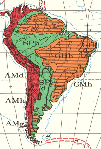
Importantly, Murphy’s criteria apply only to landforms produced by natural endogenic and exogenic processes, incorporating the driving forces behind their genesis, the resulting form they took, and their modification by natural processes, all at regional physiographic scales. He did not include any measure of human modification of landforms. Although still more impactful at local rather than regional scales, humans are today extensively modifying the geomorphology of landscapes such that sociocultural forces should now be considered along with natural forces for a more complete understanding of the distribution of landforms on the planet (Tarolli et al. 2019). Incorporating human activity as an important modifier of natural landforms (anthropogenic geomorphology) is challenging, however, and beyond the scope of this analysis. An example of the cartographic presentation for Murphy’s (1968) Landforms of the World map is shown in Figure 1.

Figure 1. Excerpt from Murphy’s (1968) map showing level of detail used to represent the landforms of South America (approximately 1:50,000,000 scale). The first uppercase letter of the three-letter landform labels refers to the structural variable: S = sedimentary covers outside shield exposures; G = Gondwana Shield; A = Alpine fold system. The second uppercase letter of the three-letter labels refers to the topographic variable: P = plains; H = hills; M = mountains. The third lowercase letter of the three-letter labels refers to the climatic or glaciation variable: h = humid; d = dry; g = Pre-Wisconsin Würm glaciation).

Bridges’s Geomorphological Divisions, Provinces, and Sections

In the preface and introduction of World Geomorphology, Bridges (1990) identified his work as a geomorphological treatment and inventory of the large-scale features of the Earth’s surface. The subsequent chapters introduce the geomorphological settings of the continents of the Earth. Bridges introduced geomorphological divisions with a rationale based on tectonic plates and predominating physiographic characteristics. For each division, provinces and sometimes sections were enumerated, each with descriptions of their physical setting, including elevation, age, and tectonic properties and their formation processes. Bridges also made an extensive effort to follow historical precedent in asserting names at each level of subdivision.

Bridges’s World Geomorphology remains the only globally consistent and comprehensive effort to delineate geomorphological divisions, provinces, and sections. Only one review (Marston 1992) exists for World Geomorphology, noting the completeness of the work, relative thinness of discussion of exogenic processes, the missed opportunity to discuss the effects of climate on landforms, and particularly the poor quality of the outline maps, which lack sufficient geographic orientation.

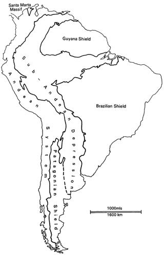
An example of one of the graphics from Bridges’s book is presented in Figure 2, showing Bridges’s divisions for South America. The graphic is reproduced at a scale and page size format that facilitates visual comparison with the Murphy’s landforms depicted in Figure 1. The similarities in the graphics visually reinforce the notion that a relationship exists between Murphy’s landforms and Bridges’s divisions, as would be expected from similarities in the conceptual nature of the two characterizations.

Figure 2. Excerpt of Figure 4.27 from World Geomorphology (Bridges 1990) showing the level of detail used to present the major geomorphological divisions of South America (approximately 1:50,000,000 scale).

Perhaps the most unexpected by-product of researching Bridges’s and Murphy’s works was noting a lack of globally comprehensive antecedents. Thus, Murphy and Bridges appear to be the first to produce globally comprehensive treatments of their respective subjects. Thrower (1968) noted that past landform classifications tended to be genetic or strictly empirical, and Murphy explicitly intended to reconcile these approaches into a single classification. In his preface, Bridges noted geomorphologists had generally avoided regional or global treatment of their subject, and he intended to be the first to produce a global work based on lithospheric plates and continents as an organizing context.

Methods

Prototype Development

The NLW2 product that we describe in this article is the outcome of a second attempt to define Bridges’s units using Murphy’s landforms. This first attempt was named World Named Landforms (Frye et al. 2018) and will be referred to herein as NLW1. The NLW1 did not include an independent recompilation of Murphy’s landforms from new source data layer inputs, and instead relied on the original Murphy’s landform polygons from his 1968 map. For that effort, ArcGIS was used to manually edit a polygon data set of world continents. The main operation was to split the continents based on a scan of Murphy’s (1968) map in the background. Bridges’s maps and descriptions were then used to further split these polygons using background layers of global elevation and lithology data sets. Each resulting polygon was assigned attributes based on Murphy’s classification and Bridges’s names. NLW1 contained 4,417 polygons, but numerous errors in the hierarchy of divisions and provinces were evident. The data from NLW1 were made available in ArcGIS Living Atlas of the World but considered as not achieving the full potential modern geographic information systems (GIS) could produce. It was decided that a recompilation approach was warranted, and that a new method be devised to automate extraction of Murphy’s landform attributes from authoritative, recently produced, globally comprehensive data sources.

Data Sources

For the recompilation of Murphy’s landforms, we used the following relatively high spatial resolution data sets:

1. Structural: Global Lithological Map (GLiM; Hartmann and Moosdorf 2012), which provides one-to-one correspondence for sedimentary areas and were interpreted to assign volcanic, shield, rifted, and alpine system classes.

2. Topographic: Hammond Landform Regions (Karagülle et al. 2017), which provided detailed classes were reduced to match Murphy’s work.

3. Erosional and depositional: A global bioclimate data set (Metzger et al. 2013) provided the basis to distinguish moist versus dry landforms, and Bridges (1990) included descriptions and maps of glaciated areas matching Murphy’s classes.

Structural Variable

The basis for the structural class is the GLiM (Hartmann and Moosdorf 2012). This data set is used in the form of a 250-m cell-size raster representing lithological classes. Thus, a challenge arises from the fact that the classes in Murphy’s Structural variable are based on rock age and hardness rather than rock type. To address this challenge, only the GLiM sedimentary class was used; other classes were grouped into a temporary class for the purposes of the initial geometric union process.

To add Murphy’s structural classes for Alpine System, Rifted Areas, Gondwana Shield, Laurasian Shield, Caledonian and Hercynian Remnants, and Rifted areas, the NLW1 was used in the same fashion as described previously and corresponding landform polygons were selected based on having their centers within each class of structural polygon in the NLW1 data set.

Two important differences between Murphy’s map and NLW1 were immediately obvious. First, sedimentary areas occurred throughout other regions. This difference was retained in NLW2 based on Murphy’s work being based more on bedrock geology and less on the surficial geology often found in the country-level compilations represented in the GLiM; Murphy (1970) indicated favoring predominance in determining shield, rifted, and alpine system regions. The second difference was the additional resolution and detail provided by the GLiM data, which introduced highly complex and often ambiguous zones where boundaries should exist between shield and rifted, and shield and alpine system classes. These boundaries were scrutinized and manually adjusted during a two-month manual editing process. Often, the values of the topographic class were used to determine the structural boundaries while visually comparing to detailed hillshaded relief maps, which often exhibited deterministic patterns of orogeny.

Similarly, volcanic areas also required intensive manual review. Murphy absorbed large areas of volcanism within the alpine system and rifted shield area structural classes, and only assigned the class of isolated volcanic areas to areas where volcanoes occur adjacent to shield areas. Thus, the locations for Murphy’s isolated volcanic areas are islands and smaller zones in Africa. The NLW2 conforms to this pattern, relying on Bridges’s province names, which identify them as such.

Topographic Variable

The basis for the topographic variable is a compilation of global Hammond Landform Regions (Karagülle et al. 2017) produced from a global 250-m digital elevation model (DEM) called GMTED 2010 (Danielson and Gesch 2011). The topographic variable in Murphy’s map also used Hammond’s classification.

The global Hammond Landform Regions data did not include Murphy’s class of depressions or basins. NLW1 included these features, however, as shown in Murphy’s original map. The boundaries for these regions were determined using the GMTED 2010 data set with hypsometric tinting to show the extent of each basin. Those in mountainous areas tended to be smaller and very clearly bounded, whereas those in generally flat areas, such as the Sahara, often had a portion of the perimeter that was more arbitrary, rather than phenomenologically determined. To assign the class of depression or basin, all NLW2 polygons with their centers within an older depression polygon were included. Each area was manually reviewed with edits applied to either change the topographic class to an adjacent value or split the polygon between the depression and the adjacent value. A hillshaded relief model was used in the background of the editing work to guide these decisions.

Murphy’s map included a Hammond class of widely spaced mountains. Karagülle et al. (2017) found, however, that using the GMTED 2010 DEM was sufficiently detailed to warrant replacing this class with either plains or mountains; that is, the class of widely spaced mountains is only valid for smaller scale maps. Thus, because the NLW2 would also be compiled at the same resolution as GMTED 2010, the widely spaced mountains class is not present.

Erosional, Depositional, and Glaciation Variable

The NLW2 uses six of the nine classes in Murphy’s erosional and depositional class, omitting three classes of offshore line features. Three sources were used, starting with GLiM, which provided locations for surficial ice. The basis for dry versus moist came from a high-resolution bioclimate map (Metzger et al. 2013), which used an aridity index to differentiate moist versus dry classes. Two sources were used as the basis for the three glaciation classes (unglaciated, Wisconsin and Würm, and pre-Wisconsin and Würm): Murphy’s map, and Bridges, who included maps of the extents of glaciation in the divisions where glaciation occurred. A similar manual editing process to that used for determining the boundaries between rifted, alpine systems, and shield structure classes was used to determine glacial boundaries. This work was complex because areas composed of older harder lithology tended to be sharpened and striated due to glaciation, whereas newer, softer areas of lithology tended to be smoothed and rounded by glaciation.

Scale

The original maps of Murphy and Bridges were small scale, about 1:50,000,000, with a range of minimum mapping units between 100 km² and 500 km²; see Figures 1 and 2. In comparison, NLW1 could support scales as large as 1:5,000,000. The recompiled Murphy’s landforms used 250-m resolution source data, considerably improving on the original spatial resolution. The minimum mapping unit of the NLW2 is 5.0 km² and the data are suitable for creating maps at scales as large as 1:500,000.

Processing

The NLW2 was produced using a series of hybrid raster and vector workflows. The general process was to produce the geometric union of global GIS data sets representing most of Murphy’s landform variables with a NLW1 data set representing Bridges’s original divisions, provinces, and sections developed from a digital capture of the graphics in his book. This geometric union follows the premise of Finch’s (1933) Fractional Code, where each resulting polygon carries the combination of the values from all input polygons.

The result of this union was a polygon data set with 2,897,842 polygons, and a large majority of these polygons were smaller than 5.0 km². Many of these small polygons occurred in coastal areas. Polygons smaller than 5.0 km² that represented offshore islands (i.e., had zero contiguous neighbors) were deleted, in keeping with a minimum mapping unit of 5.0 km². This removed 1,145,345 polygons from the initial result while retaining 1,752,497 polygons.

Next, an iterative aggregation generalization workflow was applied (Table 1). The adjacent neighbors of each remaining polygon of less than 5.0 km² were selected based on the length of shared perimeters to conditionally determine the largest compatible neighbor. Then each small polygon was dissolved into that neighboring polygon. Six iterations of this workflow were used, starting with polygons smaller than 1.0 km², then increasing in size to 2.0, 4.0, 16.0, 25.0, and 125.0 km². This reduced the number of polygons to 77,287. The intention for this progressive set of iterations was to avoid eliminating small polygons that should coalesce into relatively small, but valid landforms. For example, a set of small polygons of hills and plains should not be absorbed arbitrarily within a much larger surrounding area of mountains when they could coalesce into a polygon of mostly hills.

Table 1. Criteria for selecting and dissolving polygon neighbors based on values of structure, topographic, and moisture variables

Iteration	Minimum size (km^2)	Criteria for compatibility	No. of polygons
0	0.0625	After removal of small incompletely defined coastal polygons	1,752,497
1	1.0	Small plains into larger hills, small hills into larger mountains, and small sedimentary into larger shield neighbors	856,152
2	2.0	Small plains into larger hills, small hills into larger mountains, and small sedimentary into larger shield neighbors	694,184
3	4.0	Small hills and plains into larger mountains and small sedimentary into larger shield or alpine neighbors	427,761
4	16.0	Any small topographic areas into larger mountains and small sedimentary into larger shield or alpine neighbors	217,069
5	25.0	Any small topographic areas into larger mountains, small sedimentary into larger shield or alpine neighbors, and small moist or dry areas where structure and topographic were the same into larger neighbors	168,750
6	125.0	Small moist or dry areas where structure and topographic are the same into larger neighbors	77,287

The conditions for each iteration were adjusted though the processing. Lesser differences in topography and structure were processed first, in part because these were the most detailed of the input variables. The conditional logic favored higher relief topographic classes; for instance, a small polygon representing hills is more compatible with mountains than plains. Also, small polygons representing plains are more compatible with neighboring hills rather than mountains or high tablelands. The final iteration only focused on the moist versus dry classes of the erosional and depositional variable because the source data were originally compiled at a resolution of 1.0 km cell size as opposed to the 250 m cell size used for the structural and topographic variables.

One additional issue was handled during the aggregation iterations: the need to address differences in the size and extent of surface waterbodies represented in the source data for the topographic and structural variables. If either source indicated surface water, and a larger neighboring polygon was also surface water, then the small polygon was aggregated as surface water. Surface water was classified in two ways. Those large waterbodies appearing on Murphy’s map, such as the Great Lakes of North America, were classified into a division of Large Inland Water Body and are not assigned to a province; there were thirty-one of these polygons. Due to the higher resolution input data used to define landforms, an additional 202 polygons representing smaller inland water bodies were retained. These small waterbodies are not given a landform code and are, however, assigned to the surrounding province and division.

The resulting data set with 77,287 polygons still lacked several classes from structural, topographic, and erosional and depositional variables. Polygon data sets representing those regions already existed in NLW1 (Frye et al. 2018) and were used to assign the missing class values to the NLW2 data set.

Throughout the processing of the NLW2 data we visually inspected each stage of our work, first in ESRI’s ArcMap and later ArcGIS Pro software. These comprehensive inspections involved evaluating specific combinations of variables in Murphy’s classes or ensuring that the expected topological structure of Bridges’s hierarchy of features remained intact throughout the workflows.

Additional Tectonic Plate and Tectonic Process Attribution

We provided additional attribution in the form of tectonic context to show how landforms overlaid or corresponded with tectonic plates and processes. Although Murphy (1970) did not specifically mention tectonic plates and processes, he did discuss orogenic processes and broadly offered a structural classification that serves to ground analysis of the basic structure of the planet in tectonic processes. Bridges (1990) frequently referred to tectonic plates and processes in discussions of provinces and sections.

For tectonic processes, we selected three that correspond well to the variables defined by Murphy and Bridges: orogenic, spreading rifts, and subduction zones. These processes generally overlap with Murphy’s (1970) broad structural classes of Alpine System, which represented the mountainous areas newer than Precambrian, and Rifted Shield Areas.

As we began the tectonic attribution work, we found the existing tectonic plate boundary GIS data sets to be coarse and only suitable for very small-scale maps. The plate edges below continental land masses often did not match the relatively detailed terrain or landform boundaries. Empirically, it seemed clear that the tectonic plate boundary data were in many locations unable to represent details equivalent to the 250-m resolution of the landform polygons. Thus, we adopted the strategy to list all tectonic plates that underlie each landform in the order of area, with the largest area first and the smallest area last.

In assigning plates to landforms, we were also aware that tectonic plates are complex three-dimensional conceptualizations that relate to adjacent tectonic plates in many ways. Thus, landforms above or near plate boundaries are merely surficial and can be dependent on or independent of the underlying tectonic plates’ circumstances.

We evaluated several GIS data sets representing tectonic plates and processes that have been produced since the 1990s.

• U.S. Geological Survey (USGS) Earthquake Science Center (USGS Earthquake Science Center 2019). No author or lineage is provided, perhaps based on Simkin et al. (2006). The quality of the polygons is very coarse.

• Bird’s (2003) “An Updated Digital Model of Plate Boundaries” published by Ahlenius (2014), username Fraxen.

• Gaba’s (2018) Tectonic Plates Boundaries World Map, a widely used cartographic illustration resulting from the author’s interpretation of several earlier works. Although far more detailed than the USGS Earthquake Science Center map, GIS data were not available in GIS format and required obtaining permission to use.

• GPlates (Müller et al. 2018) is a model for visualizing plate tectonics. The corresponding GIS data did not match well with any of the other plate boundary data.

• New Maps of Global Geological Provinces and Tectonic Plates (Hasterok et al. 2022) provides inventory and discussion of recent work to map tectonic plates, but the licensing did not permit creating or distributing updates.

• Tectonic Map of the World (Bally 2007) is a collection of GIS layers produced by the American Association of Petroleum Geologists (AAPG). Although this collection is in the public domain, similar to GPlates, these data did not match well with detailed relief and bathymetry.

We selected the 2014 compilation of Bird’s work (Ahlenius 2014) on which to base our work. Our attribution work was completed in two phases: Assign plate(s) then assign processes. The plates were assigned in two phases:

1. Any landform completely inside a plate was assigned a plate_1 field value matching the plate name.

2. All other landforms were overlapped by two and up to five tectonic plates and we assigned fields in the order of the size of overlap, such that plate_1 was the largest overlap, plate_2 was the next largest, and so on.

The horizontal correspondence of Ahlenius’s polygons was not perfectly suited for our purpose and we found and updated numerous plate boundary locations to better match detailed terrain, lithology, or bathymetry data. We also checked more recently published corroborating research for each such change. Two significant changes were made to Ahlenius’s data: We subdivided the Eurasian and African plates to represent the Adriatic and Sinai microplates.

The complexity of orogenic, spreading rifts, and subduction zones over the period of geologic time from the Cambrian through the Neogene periods allowed for the potential to have two or more tectonic processes to have occurred. We represented the one process that most likely produced the basic shape; that is, enduring topographic character of each landform. It was also possible that the same process (e.g., orogenic) could have occurred multiple times during the existence of the landform but might not currently be occurring. Thus, subduction and orogenic assignment could refer to ancient or active processes; one example of this is the Ural Mountains.

Additionally, we found Bridges frequently referred to areas within divisions and provinces as being formed by one of these processes, for example the Rhine Rift Valley within the Scarplands in Bridges’s Figure 8.18. There are many instances of tectonic processes smaller than landforms as defined by Murphy’s method, however, such as the Lozoya Rift in the Central Cordilleras of Spain, which we could not definitively locate based on Figure 8.27 in Bridges.

Manual Editing to Adjust Bridges’s Unit Boundaries

The geometric union of the original, relatively coarse Bridges units with the recompiled, relatively fine Murphy’s units necessarily produced splits in many of the new landform polygons and artifactual slivers at the edges. Reviewing and fixing these slivers and splits required a month of manual editing, moving division by division through the world. The main task was finding apparent discontinuities caused by the NLW1 Bridges features in otherwise natural appearing detailed NLW2 landform polygons. Whenever the landform classes matched, usually for the sliver case, the adjacent pairs of polygons were merged.

Similar to the need to accommodate smaller water bodies, 1,350 smaller islands larger than 5.0 km² existed. These were given an arbitrary division of Island.

This manual editing process reduced the count of polygons from 77,287 to 53,965. Due to several discontinuities in World Geomorphology, there are additional provinces in the NLW2, including one for small islands, and another for major inland water bodies, which corresponds with Murphy’s map. One exception is Antarctica. Although Bridges and Murphy treated the southernmost continent, the data sets used to derive the NLW2 did not.

Coastline Adjustments

The coastlines for the GliM, Hammond Landform Regions, and bioclimates differed substantially, and frequently resulted in missing values for one or two variables in the 250-m raster cells along the coasts. For bioclimates and GLiM this meant presuming values based on adjacent values. For example, a narrow landform polygon representing a thin stretch of coastline, lacking a value of dry or moist, could be absorbed into the neighboring landform.

Generally, the best coastline representation came from the Hammond Landform Regions. This coastline does not conform well, however, to more detailed coastlines commonly available in online base maps or to authoritative data (e.g., Sayre et al. 2019). Additional time was therefore dedicated to manually editing the coastlines, particularly near populated areas, to improve their alignment with more detailed coasts. Complex coastal areas such as the southern extent of South America were not undertaken.

Results

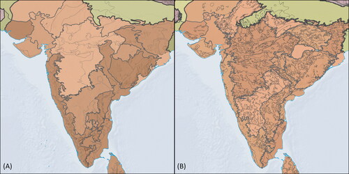
An example of the map outputs from NLW1 and the subsequent NLW2 is shown in Figure 3. Comparing the relative sparseness of interior landform boundaries in NLW1 to the richer collection of landforms in NLW2 shows the improvement in spatial resolution that was obtained using the automated workflow.

Figure 3. (A) Named Landforms of the World, version 1.0 at scale of 1:20,000,000 based on a manual editing workflow showing division, province, and landform boundaries of India. (B) Improved Named Landforms of the World, version 2.0 at scale of 1:20,000,000 based on an automated workflow showing greater detail and precision of division, province, and landform boundaries of India.

The NLW2 contains 53,947 polygons. It includes 425 geomorphological provinces within fifty-three divisions; there are 138 sections within forty-four of the provinces. An example of the cartographic treatment developed for the NLW2 is provided in Figures 4, 5, and 6. Figure 4 depicts the global distribution of Bridges’s geomorphological divisions, and Figure 5 shows those same Bridges’ divisions subdivided by provinces.

Figure 4. Bridges’s Geomorphological Divisions (53) reconstructed from Murphy’s Landforms.

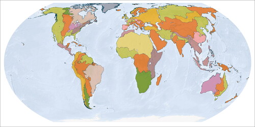
Figure 5. Bridges’s Geomorphological Provinces (425) as subdivisions of the fifty-three Geomorphological Divisions depicted in Figure 4.

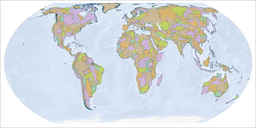
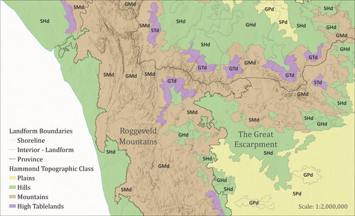
Figure 6. Example of Named Landforms of the World, version 2.0 showing recompiled Murphy’s landforms and their contribution to the definition of named provinces. The thickest black lines indicate province boundaries. The location is on the west coast of South Africa where three provinces meet. The landforms are labeled by codes representing each of Murphy’s variables: S = sedimentary covers; G = Gondwana Shield areas; H = hills; M = mountains; T = high tablelands; P = Plains; d = dry landform areas.

Geodesic area calculations for the NLW2’s units and variable classes are shown in Tables 2 through 5.

Table 2. Areal composition of Bridges units in Named Landforms of the World, version 2.0 as the proportion of the world’s land surface (excluding Antarctica) that are covered

Bridges unit	Area (km^2)	Global % of land
Divisions	132,177,276.1	98.43
Provinces	121,461,459.3	90.45
Sections	13,812,817.0	10.28

Note: These figures do not include polygons assigned a generic division of major inland water body or island, which accounts for the 1.57 percent of land not covered by an area included in a Bridges (1990) division.

Table 3. Areal composition (excluding Antarctica and surface waterbodies) of Murphy’s landform variables and classes in Named Landforms of the World, version 2.0

Variable	Landform code letter—Class name	Area (km^2)	% of land
Structure	A—Alpine fold system	29,827,033	22.58
	C—Caledonian and Hercynian (or Appalachian) remnants	4,416,462	3.33
	G—Gondwana Shield	15,372,368	11.64
	V—Isolated volcanic areas	304,196	0.23
	L—Laurasian shields	7,265,656	5.50
	R—Rifted shield areas	2,077,378	1.57
	S—Sedimentary covers outside shield exposures	72,793,925	55.12
Topographic	P—Plains	53,238,546	40.31
	H—Hills and low tablelands	32,123,503	24.32
	M—Mountains	43,009,431	32.56
	T—High tablelands	1,091,688	0.82
	D—Depressions or basins	2,593,850	1.96
Glaciation	“”—Not glaciated	101,608,894	76.94
	g—Pre-Wisconsin Würm	12,523,595	9.48
	w—Wisconsin Würm	17,924,530	13.78
Moist or dry	m—Moist	53,045,143	40.16
	d—Dry	77,325,287	58.55
	i—Ice	1,686,589	0.58

Table 4. The ten largest landform types, of the 142 that occurred, which account for 64.94 percent of the land surface of the Earth (excluding Antarctica and surface waterbodies)

Landform code	Area (km^2)	Global % of land
SPd	23,628,327	17.89
Amh	12,199,544	9.23
SPh	11,564,541	8.75
Amd	7,217,378	5.46
SHh	7,216,902	5.46
SHd	6,771,347	5.12
GHh	5,269,982	3.99
SPgh	4,948,964	3.74
SPwh	4,003,397	3.03
GMh	2,922,880	2.21

Note: Landform codes are formed by the sequence of structure, topographic, glaciation, and moist or dry letters shown in Table 3. Globally, dry sedimentary plains are the most extensively occurring landform, occupying approximately 18 percent of the Earth’s terrestrial surface.

Table 5. Areal composition (excluding Antarctica and surface waterbodies) of tectonic process variable

Landform code	Area (km^2)	Global % of land
Orogenic	26,246,696	19.88
Rift zone	17,037,926	12.90
Above subducting plate	18,287,669	13.85
None	70,484,726	53.37

The landform regions in the NLW2 are defined by the same three variables Murphy used, but at a higher resolution that provides the capacity to distinguish single landform features, as illustrated in Figure 6. This is mainly determined by the topographic variable. The data sources for structural and erosional and depositional characteristics are not as detailed. Although the GLiM is detailed, the classes of lithology are broad, and although regions have detailed edges, they tend to be much larger in area. The count of polygons in each class of variable (Table 6) illustrates the relative differences in level of detail.

Table 6. Area and count of Named Landforms of the World, version 2.0, polygons by landform variable

Murphy variable	Polygon count	Average area (km^2)	No. of unique values
Topographic	26,521	5,078.2	6
Structural	10,885	12,372.9	8
Erosional and depositional	3,851	34,972.5	8

Discussion

As expected, the automated recompilation of Murphy’s landforms from independent data layers representing structural, topographic, and climatic and weathering variables produced a finer spatial resolution data layer with considerably richer geographic detail than the original hand-drawn rendering. These landform polygons proved to be a good basis to assign Bridges’s division, province, and section names. Many details of this work were not straightforward, and in fact the digital reconstruction and spatial reconciliation of the two resources was often arduous and time consuming, requiring considerable manual editing. In the process, many issues arose that required careful thought and extra editing attention. We discuss four of these issues next, followed by a discussion of the accuracy, utility, and opportunities for future improvement of the work.

Discrete Landform Features vs. Landform Regions

Murphy adhered to a principle of predominance when describing a region as having similar structure, topography, and erosional and depositional character. Today, global high-resolution hillshaded terrain maps are widely available. These relief depictions show individual landform features and regions of similar terrain at many different scales. These higher resolution products might make it seem like Murphy’s small-scale map is dated because readers can now easily zoom to larger scales and discern smaller regions and individual landform features (i.e., one mountain, hill, or plateau). For example, a region that Murphy’s map describes as plains might contain a mountain or mountains, which are discernible only from high-resolution shaded relief data. The land surface for most of the region, however, is predominantly flat, and was therefore designated as a plains landform.

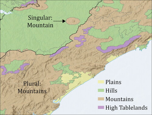
Against this backdrop, the singular feature on the earth definitions for landform are not adequate. Murphy’s use of the term landform encompasses a predominant local feature and a group or region primarily composed of similar features. Thus, a single mountain is a landform, as is a group of hills formed by a glacier’s terminal moraine. Further, landforms include terrain that is within the influence of a dominant feature or type of feature. A large mountain includes toe slopes, flat river valleys between ridges, and even plains that fall within the shadow of the mountain. Körner, Urbach, and Paulsen (2021) asserted a similar view regarding the definition of a mountain including and influencing adjacent space. Similarly, regions of hills include small areas of flat plains or low tablelands between hills. This distinction between landforms as discrete, singular features and landform regions consisting of multiple similar features is illustrated in Figure 7.

Figure 7. Example showing the area around São Paulo, Brazil, with singular landform features in the common sense and plural landform regions where a topographical class predominates (approximately 1:2,000,000 scale).

Suitability of Murphy’s Landforms for Bounding Bridges’s Units

As described in the methodology, when a division, province, or section as defined by Bridges required a landform to be split, Murphy’s variables were identical for the pair of polygons on either side of the split. We evaluated the division, province, and section boundaries to determine whether the adjacent pairs of polygons had identical versus at least one different value for any of Murphy’s three variables. Based on this evaluation, we found 85.34 percent of the length of division, province, and section boundaries were determined by Murphy’s landforms. Generally, when the boundaries for Bridges’s units were not determined by landforms, they were split based on independent criteria such as elevation or visual variation of terrain morphology within a particular topographic class. In some cases, particularly in the Sahara and the desert regions of Australia, these boundaries were based solely on Bridges’s original line maps.

The combination of Murphy’s landforms with Bridges’s units is not a new classification. Murphy asserted that his landform classification, which in its essence is an exogenic description, could be readily used for genetic explanation (Thrower 1968). We expected Bridges’s units, which are richly endogenic and genetic would be a suitable match. The 85.34 percent of shared boundary matches strongly supports our expectations.

Underrepresentation of High Tablelands

In the development of the global Hammond landform regions (Karagülle et al. 2017), which were used to reconstruct Murphy’s topographic variable, different minimum mapping units and raster processing neighborhood analysis window sizes were used for the different landform types (plains, hills, mountains, and tablelands). Plains and high tablelands were empirically determined to have the smallest minimum detectable areas, whereas a larger area was required to define a hill, and a still larger area for defining a mountain. In the case of tablelands, the resolution of the DEM affects the algorithm. The 250-m GMTED DEM (Danielson and Gesch 2011) identified tablelands of a specific size range (Karagülle et al. 2017). Although a finer resolution DEM could be used to identify smaller buttes and plateaus, another issue exists: The elevation values represented by each cell in a DEM are an average of elevation values. This average for a 250-m cell could represent a flat plain or very rough or eroded terrain. The larger the cell size, the more likely rough surfaces could be evaluated as flat tops of plateaus, versus high hills or mountains. Thus, the complete inventory of the world’s tablelands is not fully represented in the work produced by Karagülle et al. (2017).

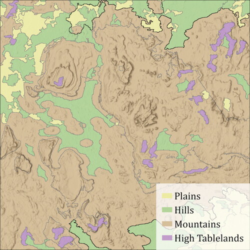
Although Murphy included a class for high tablelands, the number of such regions was very small. This is in part due to the small scale of Murphy’s map, which could not represent relatively small tableland features. During the manual review and editing of the NLW2, it was observed that although many additional areas of high tablelands were identified relative to Murphy’s original map, these highland regions often seemed fragmented and incomplete. Thus, we consider high tablelands underrepresented in the NLW2. This underrepresentation of highlands is well illustrated in the Guiana Highlands (Figure 8).

Figure 8. In this area of the Guiana Highlands, only a small portion of the high tablelands were identified in purple by Karagülle et al. (2017), and instead many tablelands were classified as mountains (approximately 1:2,500,000 scale).

Inconsistencies in Bridges’s Unit Descriptions and Delineations

In compiling the NLW2, many inconsistencies were noted in the text and graphics in World Geomorphology. At times what was presented in the text was not reflected in or at odds with what was presented in the accompanying graphics. At other times Bridges’s introductory materials conflicted with the details presented in the full descriptions within the chapters. The maps often appear to have been compiled at differing stages of the editorial process, showing Bridges was wrestling with the relationship of parts to wholes at all levels of the hierarchy. In developing the NLW2, we prioritized the generally richer detail provided in Bridges’s full descriptions for sections, provinces, and divisions over the summary introductions of the chapters and the maps, particularly those maps at smaller scales.

Accuracy, Utility, and Opportunities for Future Improvement of the NLW2

A traditional quantitative accuracy assessment for quantifying the quality of the NLW2 as a digital reconstruction and spatial combination of two qualitative historical works was not considered feasible or appropriate and was therefore not attempted. This was primarily due to the lack of a “gold standard” global geomorphological data layer to use as the reference (truth) for comparison.

Detailed work such as Marshall’s (2007) chapter, “Geomorphology and Physiographic Provinces of Central America,” illustrates how the NLW2 is needed and could be improved. The need is based on Marshall’s work lacking an overview map showing all provinces and doing so in the context of bordering divisions and provinces. Yet, Marshall’s work is newer, arguably better informed, and topologically different than Bridges. Although it appears that Murphy’s landforms could be reaggregated to reflect Marshall’s provinces, even without doing so the NLW2 provides valuable regional, continental, and global-scale context for better understanding Marshall’s units.

Murphy (1970) described his rule for the structural class of isolated volcanic areas to only include those volcanic areas “lying outside the Alpine or older orogenic systems, and outside the rifted shield areas.” This rule left many volcanic areas, such as the majority of the Aleutian Islands, generically within the Alpine System class, but only covering small portions of those regions. Using volcano locations (Venzke 2013), we determined that approximately half of all landforms containing volcanoes are not classified as such, including many large volcanic zones such as those in the southern Andes mountains, the Caribbean, or southern Mexico. Given the finer resolution of landforms in the NLW2, it is possible to assign volcanos and volcanic areas as subclasses within alpine systems and rifted shield areas or within the topographic class. Characteristics such as age and whether a volcano is active seem useful as future attribution work to improve the NLW2.

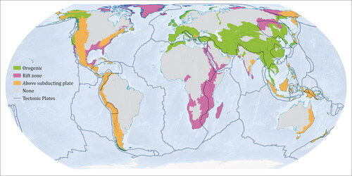
In assigning the plate tectonic processes of Orogenic, Rift Zone, and Above Subducting Plate to the landforms of the NLW2, it was found they predominated within Murphy’s structural classes of Alpine System, and Caledonian and Hercynian Remnants. Figure 9 illustrates the global distribution of these tectonic processes. Although the landforms of the NLW2 generally represent the area of tectonic processes well, there are several areas, such as the west coast of North America, where complex interactions between plates relate poorly to topography.

Figure 9. Deterministic tectonic processes for landforms (1:200,000,000 scale).

Another future improvement of the NLW2 would be to better distinguish the numerous exogenic processes such as glacial scouring and moraines, eolian and fluvial erosion and deposition, subsidence, earthquakes, and so on, that modify landforms subsequent to their genesis. This is consistent with the criticism by Marston (1992) that Bridges’s characterizations were notable in the lack of a treatment of exogenic processes. In the future, a stronger incorporation of both exogenic natural drivers of landform development and even human drivers of landform development (Tarolli et al. 2019) would be desirable.

In evaluating landforms based on the tectonic process of rift zone and Murphy’s structural class of rifted shield, we found two areas of discrepancy. Murphy (1970) noted the Lake Vaatern vicinity in Sweden and the Flinders area of southern Australia as being rifted shield, yet neither are associated with a tectonic plate edge. Both areas can be described as associated with normal continental faulting that typically produces horsts and grabens. The AAPG published The Tectonic Map of the World (Bally 2007), which includes a polygon data set of 589 rifted areas that intersect areas representing all of Murphy’s structural classes. Future work to determine which landforms correspond with such continental faulting activity would be helpful to further delineate these features.

Finally, after systematically expressing Bridges’s work in the NLW2, an important question is whether all divisions must be divided into provinces, and then all provinces into sections to complete a hierarchical tessellation. There were many opportunities to add sections within many provinces where Bridges did not do so. Yet, Bridges implied this general intention, based on Fenneman (1916), to globally provide a first order of continents, a second of divisions, and a third order of provinces. Bridges also asserted that a fourth level of sections logically follows. Although Bridges gave the example of the Black Hills in the western portions of the states of North and South Dakota, the provinces and sections provided in his chapter on North America do not comprehensively cover the continent. Despite stating the capacity to produce this fourth level of detail, Bridges did not generally do so, and this remains as work to be undertaken in the future.

Conclusion

We produced a scientifically rigorous, hierarchical, data-derived, globally comprehensive, and standardized map of Named Landforms of the World. To do so, we first updated Murphy’s original landforms, which although conceptually rigorous, were delineated by hand based on a broadly interpretive approach. We recompiled Murphy’s landforms using a fine-grained, data-derived approach made possible by GIS and the availability of detailed geomorphic information. Our approach was to spatially combine best available data layers representing each of the three inputs (structural, topographic, and climatic or glaciation). We then aggregated these updated Murphy’s landform polygons into the larger Bridges’s geomorphological divisions, provinces, and sections. Thus, we sought to reprise Bridges’s original, coarsely sketched geomorphological regions, with more finely grained, empirically defined regions based on the aggregation of Murphy’s landform regions.

The NLW2 offers improved representations of land surface characteristics that can support development of spatial frameworks to represent ecological regions, habitat, and conservation and agricultural priorities. Averages by landform type of biomass, soil moisture, crop yield, and so on, and inventories of species composition and population density can support land managers and policymakers by augmenting functional understanding of local landscapes. Hora, Almonacid, and González-Reyes (2022) provided an example of topographic character providing ecologically useful distinctions. The NLW2 could also serve as a basis to inventory occurrences of geologic hazards, such as mass wasting events.

Independent of the NLW2, there are a number of studies (e.g., the Marshall [2007] analysis referenced earlier) that illustrate the wide variety of compilation methods and mapping techniques used in geomorphological analysis. This diversity in approaches is well illustrated in the Springer multivolume series World Geomorphological Landscapes (Migon 2022), a compendium of national studies that vary considerably in nature and derivation. Our approach was to produce a standardized and globally comprehensive treatment of landform regions, and an additional effort to undertake an exhaustive survey of geomorphological mapping methods was considered out of scope.

Although sophisticated in conceptual and methodological treatment, the NLW2 harkens back to the work of Raisz (1957), Lobeck (1921), and especially, Fenneman’s (1916) foundational work to describe the physiographic divisions of the United States. Fenneman justified the need for his map as follows:

Official surveys, State and National, are annually describing a large number of small areas. In most cases some attention is given to the geographic setting of such areas and to physiographic description or explanation. … In describing a quadrangle, county, or other area, it is common to refer it to some larger area, generally called a province. … The implication of this, beside merely locating the field, is that the province is recognized as having certain characteristics and that in locating the field within it, a general impression of the character of the smaller area is imparted. The province, with its known characteristics, is mentioned chiefly to give a setting for the smaller field.

The NLW2 is also more than the vision promulgated by Fenneman and more than the work of Murphy and Bridges, however. The NLW2 is a starting place for globally organizing and mapping geomorphology. The NLW2 represents the familiar shapes of the Earth’s topography while cataloging the characteristics such as those defined by Murphy and Bridges. The NLW2 also represents a comprehensive framework for contextualizing modern geomorphological characterizations and studies. As we added tectonic information, the research demonstrated and confirmed Bridges’s unit names and descriptions as generally enduring the test of time over the past three decades. There are several more additions and refinements needed before the NLW2 can realize a broader vision:

• Expansion of how volcanos are represented as landforms.

• More detailed treatment of glaciation, including additional ages and distinguishing of moraines and scouring processes.

• Addition of an attribute for the geologic age for when a given landform was best estimated to have been formed. For example, this would allow glacial or volcanic features to be further distinguished from surrounding features.

• Most exogenic processes are underrepresented.

• A portion of the division and province boundaries remain a best guess given the coarseness and lack of context of Bridges’s line maps. Particularly, the southern portion of South America, the northern Rockies, northeast Asia, and central Australia could benefit from attention by regional specialists.

• Bridges’s first order of division was continents; perhaps tectonic plate would represent a better highest order concept.

There is therefore much additional work to be done before such a foundation can be considered complete. Despite these shortcomings, the NLW2 is currently the best available global expression of the ideas of Fenneman, Lobeck, Raisz, Murphy, and Bridges. The NLW2 now permits the query of any location on Earth, returning richly detailed geomorphological attribute information not heretofore available. We offer the NLW2 as a conceptually and geographically comprehensive resource with value as an emerging global framework for organizing geomorphological studies.

Acknowledgments

Any use of trade, product, or firm names is for descriptive purposes only and does not imply endorsement by the U.S. Government. The authors are grateful for the journal-provided reviews and for helpful comments from Greg Snyder of the U.S. Geological Survey.

Additional information

Notes on contributors

Charlie Frye

CHARLIE FRYE is Chief Cartographer at ESRI in Redlands, CA 92373. E-mail: [email protected]. His research interests include cartographic data modeling, representing physiography and toponyms on maps, and modeling gridded population, uncertainty, and ecosystems.

Roger Sayre

ROGER SAYRE is a Senior Scientist for Ecosystems at the U.S. Geological Survey in Reston, VA 20192. E-mail: [email protected]. His research interests are focused on the delineation of standardized global ecosystem maps for terrestrial, freshwater, and marine environments.

Alexander B. Murphy

ALEXANDER B. MURPHY is a former president of the American Association of Geographers and Professor Emeritus at the University of Oregon, Eugene, OR 97403. E-mail: [email protected]. His writings include efforts to expand understanding of the importance of geographic perspectives and representations for understanding political and environmental systems.

Deniz Karagülle

DENIZ KARAGÜLLE is a Senior Product Engineer on ESRI’s Living Atlas of the World Team in Redlands, CA 92373. E-mail: [email protected]. Her interests are in cartographic data modeling, ecosystems, landforms, urban design, and automating and mapping near-real-time data.

Moira Pippi

MOIRA PIPPI is a Master’s Student studying geological science and technology at the University of Siena, Siena, 53021, Italy. E-mail: [email protected]. In 2022, she worked as a summer intern at ESRI and contributed the tectonic plate and process attributes to this work. Her research interests also include geomorphology and volcanology.

Mark Gilbert

MARK GILBERT is a Senior Product Engineer on ESRI’s Living Atlas of the World Team in Redlands, CA 92373. E-mail: [email protected]. His interests lie in spatial data science and using programming to automate GIS workflows.

Jaynya W. Richards

JAYNYA W. RICHARDS is a Product Engineer II on ESRI’s Living Atlas of the World Team in Redlands, CA 92373. E-mail: [email protected]. Her interests include the pursuit of creative expression through the cartographic representation of beautiful and diverse cultural geography, physical natural history, multilingual etymology, and scientific observations of our diverse world.

References

- Ahlenius, H. 2014. World tectonic plates and boundaries. Accessed December 22, 2021. https://github.com/fraxen/tectonicplates.
- Bailey, R. 2014. Ecoregions—The ecosystem geography of the oceans and continents. 2nd ed. New York: Springer.
- Bally, A. W. 2007. Tectonic map of the world. Accessed April 5, 2022. https://www.datapages.com/gis-map-publishing-program/gis-open-files/global-framework/tectonic-map-of-the-world-2007.
- Bird, P. 2003. An updated digital model of plate boundaries. Geochemistry, Geophysics, Geosystems 4 (3):1–46. doi: 10.1029/2001GC000252.
- Bishop, M. P., L. A. James, J. F. Shroder, and S. J. Walsh. 2012. Geospatial technologies and digital geomorphological mapping: Concepts, issues, and research. Geomorphology 137 (1):5–26. doi: 10.1016/j.geomorph.2011.06.027.
- Bridges, E. M. 1990. World geomorphology. Cambridge, UK: Cambridge University Press. doi: 10.1017/CBO9781139170154.
- Danielson, J. J., and D. B. Gesch. 2011. Global multi-resolution terrain elevation data 2010 (GMTED2010). U.S. Geological Survey OpenFile Report 2011–1073. doi: 10.3133/ofr20111073.
- Davis, W. M. 1899. The geographical cycle. The Geographical Journal 14 (5):481. doi: 10.2307/1774538.
- Fenneman, N. 1916. Physiographic divisions of the United States. Annals of the Association of American Geographers 6 (1):19–98. doi: 10.1080/00045601609357047.
- Finch, V. C. 1933. Geographic surveying, and Montfort: A study in landscape types in southwestern Wisconsin. Geographic Society of Chicago Bulletin 9:6–40.
- Frye, C., R. Sayre, D. R. Soller, and D. Karagülle. 2018. World named landforms. Accessed December 22, 2021. doi: 10.13140/RG.2.2.31340.21129.
- Gaba, E. 2018. Tectonic plates boundaries World Map Wt 180degE centered-en.svg. Accessed June 2, 2022. https://en.wikipedia.org/wiki/File:Tectonic_plates_boundaries_World_map_Wt_180degE_centered-en.svg.
- Groves, C. 2003. Drafting a conservation blueprint: A practitioner’s guide to planning for biodiversity. Washington, DC: Island.
- Hammond, H. E. 1954. Small-scale continental landform maps. Annals of the Association of American Geographers 44 (1):33–42. doi: 10.1080/00045605409352120.
- Hammond, H. E. 1964. Classes of land surface form in the forty-eight states, USA. Annals of the Association of American Geographers 54 (1):11–19. doi: 10.1111/j.1467-8306.1964.tb00470.x.
- Hartmann, J., and N. Moosdorf. 2012. The new global lithological map database GLiM: A representation of rock properties at the Earth surface. Geochemistry, Geophysics, Geosystems 13 (12):1–37. doi: 10.1029/2012GC004370.
- Hasterok, D., J. A. Halpin, A. S. Collins, M. Hand, C. Kreemer, M. G. Gard, and S. Glorie. 2022. New maps of global geological provinces and tectonic plates. Earth-Science Reviews 231:104069. doi: 10.1016/j.earscirev.2022.104069.
- Hora, B., F. Almonacid, and A. González-Reyes. 2022. Unraveling the differences in landcover patterns in high mountains and low mountain environments within the valdivian temperate rainforest Biome in Chile. Land 11 (12):2264. doi: 10.3390/land11122264.
- Karagülle, D., C. Frye, R. Sayre, S. Breyer, P. Aniello, R. Vaughan, and D. Wright. 2017. Modeling global Hammond landform regions from 250‐m elevation data. Transactions in GIS 21 (5):1040–60. doi: 10.1111/tgis.12265.
- Körner, C., D. Urbach, and J. Paulsen. 2021. Mountain definitions and their consequences. Alpine Botany 131 (2):213–17. doi: 10.1007/s00035-021-00265-8.
- Lobeck, A. K. 1921. A physiographic diagram of the United States. Chicago: A. J. Nystrom & Co.
- Lobeck, A. K. 1924. Block diagrams: And other graphic methods used in geography. New York: Wiley.
- Marshall, J. S. 2007. The geomorphological and physiographic provinces of Central America. In Central America; Geology, resource, hazards, ed. J. Bundschuh and G. E. Alvarado, Vol. 1, 75–122. London and New York: Taylor & Francis.
- Marston, R. A. 1992. World geomorphology: Reviews and materials received. Journal of Geography 91 (1):43–50. doi: 10.1080/00221349208979338.
- Metzger, M. J., R. G. H. Bunce, R. H. G. Jongman, R. Sayre, A. Trabucco, and R. Zomer. 2013. A high-resolution bioclimate map of the world: A unifying framework for global biodiversity research and monitoring. Global Ecology and Biogeography 22 (5):630–38. doi: 10.1111/geb.12022.
- Migon, P. 2022. World geomorphological landscapes. Accessed December 14, 2022. https://www.springer.com/series/10852.
- Müller, R. D., J. Cannon, X. Qin, R. J. Watson, M. Gurnis, S. Williams, T. Pfaffelmoser, M. Seton, S. H. J. Russell, and S. Zahirovic. 2018. GPlates: Building a virtual Earth through deep time. Geochemistry, Geophysics, Geosystems 19 (7):2243–61. doi: 10.1029/2018GC007584.
- Murphy, R. E. 1968. Map supplement No. 9: Landforms of the world. Annals of the Association of American Geographers 58 (1), eds. J. E. Spencer and J. W. Thrower. Drawn by J. A. Bateman, AAG Staff Cartographer. doi: 10.1111/j.1467-8306.1968.tb01643.x.
- Murphy, R. E. 1970. Structural landform regions of the world. Proceedings of the Association of American Geographers 3:122–27.
- Murphy, R. E. 1973. Regions of erosional and depositional landforms. The Science Reports of the Tohoku University, 7th series, Geography, 213–20. Accessed December 21, 2020. http://hdl.handle.net/10097/44936.
- National Geographic Society. 2022. Resource library encyclopaedia entry lor Landform. Accessed August 2, 2022. https://education.nationalgeographic.org/resource/landform.
- Raisz, E. 1931. The physiographic method of representing scenery on maps. Geographical Review 21 (2):297. doi: 10.2307/209281.
- Raisz, E. 1957. Landforms of the United States: To accompany Atwood’s physiographic provinces. 6th ed., rev. Cambridge, MA: Erwin Raisz.
- Sayre, R., S. Noble, S. Hamann, R. Smith, D. Wright, S. Breyer, K. Butler, K. Van Graafeiland, C. Frye, D. Karagülle, et al. 2019. A new 30 meter resolution global shoreline vector and associated global islands database for the development of standardized ecological coastal units. Journal of Operational Oceanography 12 (Suppl. 2):S47–S56. doi: 10.1080/1755876X.2018.1529714.
- Simkin, T., R. I. Tilling, P. R. Vogt, S. H. Kirby, P. Kimberly, and D. B. Stewart. 2006. This dynamic planet: World map of volcanoes, earthquakes, impact craters, and plate tectonics Accessed June 2, 2022. doi: 10.3133/i2800.
- Tarolli, P., W. Cao, G. Sofia, D. Evans, and E. Ellis. 2019. From features to fingerprints: A general diagnostic framework for anthropogenic geomorphology. Progress in Physical Geography: Earth and Environment 43 (1):95–128. doi: 10.1177/0309133318825284.
- Thrower, N. J. W. 1968. Annals map supplement number nine landforms of the world. Annals of the Association of American Geographers 58 (1):198–200. doi: 10.1111/j.1467-8306.1968.tb01643.x.
- USGS Earthquake Science Center. 2019. Tectonic plates of the earth. Accessed June 2, 2022. https://www.usgs.gov/media/images/tectonic-plates-earth.
- Venzke, E., ed. 2013. Volcanoes of the world, v. 4.11.0. Smithsonian Institution, Global Volcanism Program. Accessed July 13, 2022. doi: 10.5479/si.GVP.VOTW4-2013.