Periodicity and Variability in Daily Activity Satisfaction: Toward a Space-Time Modeling of Subjective Well-Being

Abstract

Understanding how geographical environments influence peoples’ subjective experiences of daily activities is of great potential for improving subjective well-being (SWB), a subject that is presently limited by a lack of available data and proper statistical methods. Focusing on Beijing and using a unique data set that linked residents’ seven-day mobility trajectories at a fine spatiotemporal resolution to their complete activity participation and momentary well-being, this article investigates the temporal dynamics of and geographical contextual effects on SWB of daily activities. We developed a unified spatial multilevel stochastic process model to simultaneously capture periodicity, stochastic dynamics, and individual heterogeneity effects. Results show that momentary SWB has a twenty-four-hour periodicity and evolves stochastically around individual equilibrium states depending on key life-circumstance variables. Migrants and low-income residents tend to have lower equilibrium states than their counterparts. Real-time air pollution exposure significantly lowers daily activity satisfaction levels, and an inverted-U-shaped relationship exists between city vibrancy and satisfaction.

理解地理环境如何影响日常行为的主观体验, 能够大大改善主观幸福感。目前, 数据和统计方法的缺乏, 限制了主观幸福感的研究。以北京为例, 本文通过一个独特的数据集, 将精细时空分辨率的居民七天流动轨迹与其行为参与和瞬时幸福感联系起来, 研究了日常行为的时间动态和地理背景对主观幸福感的影响。我们开发了一个空间多层次随机过程模型, 同时获取了周期性、随机变化和个体异质性效应。结果表明, 瞬时主观幸福感具有二十四小时周期性, 并随着生活环境的主要变量而围绕着个体平衡状态随机演化。移民和低收入居民的平衡状态往往低于其他人群。实时空气污染暴露显著降低了日常行为的满意度, 城市活力和满意度之间存在倒U型关系。

Llegar a entender cómo influyen los entornos geográficos las experiencias subjetivas en las actividades cotidianas de las personas proyecta un alto potencial para el mejoramiento del bienestar subjetivo (SWB), tema limitado en la actualidad por la falta de datos disponibles y de métodos estadísticos adecuados. Centrándonos en Beijing, y usando un conjunto único de datos que vincula las trayectorias de movilidad durante siete días en los residentes, a una resolución espaciotemporal fina, con su participación completa en la actividad y su bienestar momentáneo, este artículo investiga la dinámica temporal y los efectos geográficos contextuales sobre el SWB de las actividades diarias. Desarrollamos un modelo de proceso estocástico multinivel espacial unificado para capturar simultáneamente la periodicidad, la dinámica estocástica y los efectos de la heterogeneidad individual. Los resultados muestran que el SWB momentáneo tiene una periodicidad de veinticuatro horas, evolucionando estocásticamente en torno a estados de equilibrio individuales, dependiendo de variables clave de las circunstancias vitales. Los migrantes y residentes de bajos ingresos tienden a exhibir estados de equilibrio más bajos que sus contrapartes. La exposición a la polución atmosférica en tiempo real reduce de modo significativo los niveles de satisfacción con la actividad diaria, y existe una relación en forma de U invertida entre la pujanza citadina y la satisfacción.

Key words:

• daily activity participation
• geographical contextual effects
• multilevel models
• space-time model
• subjective well-being

关键词:

• 地理背景影响
• 多层次模型
• 时空模型
• 主观幸福感。

Palabras clave:

• bienestar subjetivo
• efectos contextuales geográficos
• modelo espaciotemporal
• modelos multinivel
• participación en las actividades diarias

How do urban residents arrange their daily activities in space and time, and how do they experience these activities, such as working, shopping, socializing, and entertainment? Does geographical microenvironment affect subjective experiences of daily activities and, if so, how? Answering these questions is of great importance for improving urban planning and individuals’ subjective well-being (SWB). Much SWB research has been focused on global life satisfaction and its associations with a wide range of individual life-circumstance variables (Diener, Oishi, and Tay 2018), but studies focusing on issues of satisfaction with respect to residents’ daily activities at a high spatiotemporal resolution and their links to immediate geographical environments are scarce. One of the reasons for this is the lack of data that integrate residents’ fine spatiotemporal granular daily mobility trajectories with their complete daily activities and associated momentary SWB. A further obstacle is the inadequacy of mathematically robust tools for modeling such integrated trajectory data and drawing valid statistical inferences on geographical contextual effects. The second concern is that individuals perform their daily activities in diverse settings, including homes, workplaces, and shops, each with distinct microenvironments that could affect activity satisfaction levels. This complexity hinders the identification of real-time geographical contextual impacts on momentary well-being.

Drawing on a framework of time geography, individuals’ daily lives are conceptualized as a continuous space-time path that comprises a sequence of activity episodes (Schwanen and Wang 2014). Geography could be linked to momentary well-being data collected by the famous day reconstruction method (DRM; Kahneman et al. 2004). Researchers have suggested that geographical contexts, such as physical urban form, can exert significant influences on subjective experiences (e.g., Brereton, Clinch, and Ferreira 2008; Ettema et al. 2010; Ettema and Schekkerman 2016; Y. Liu, Dijst, and Geertman 2017). Urban form-related indicators, such as population density, land-use mix, road network design, accessibility to various facilities, and proximity to public transit, have been demonstrated to be associated with life satisfaction or SWB (Leyden, Goldberg, and Michelbach 2011; Morrison 2011; Birenboim 2018; Ma et al. 2018). Much research argued that people living in neighborhoods with high density, mixed land use, and high accessibility to diverse services and green space tended to have high levels of well-being, whereas some other studies had different or even opposite findings (Ambrey and Fleming 2014; Cao 2016; H. Dong and Qin 2017; Ta et al. 2021). In addition, urban vibrancy has been demonstrated to be linked with physical urban form and socioeconomic activities, and is likely to exert positive influence on SWB and quality of life (Mouratidis and Poortinga 2020; Ma, Rao, et al. 2020). Most prior studies focused on various types of geographical environment at the residential neighborhood or city scale, but little research has been conducted on the potential nexus among immediate geographical contexts at the activity episode level, situational activity characteristics, and momentary well-being (MacKerron and Mourato 2013; Doherty, Lemieux, and Canally 2014; Schwanen and Wang 2014; G. Dong et al. 2018), despite its high policy relevance to urban planning, environmental management, and quality of life.

Moreover, environmental pollution has received much attention recently and has been found to be posing significant risks to people’s health and well-being (e.g., Brink 2011; Nieuwenhuijsen 2016; Ma, Tao, et al. 2020). Some studies have suggested that environmental pollution, such as air pollution, could directly lower people’s SWB levels through the awareness of pollution exposure and its adverse effect on health (Welsch 2006; MacKerron and Mourato 2013). In most prior studies, though, environmental pollution like air pollutant concentration was mainly measured in residential places, which failed to take into account the spatiotemporal variations in pollution levels across various activity locations. As people conduct multiple activities in different places outside residences, an incomplete consideration of pollution at the residential neighborhood cannot reflect real pollution exposure that people experience during their daily lives (Yoo et al. 2015; Kwan 2018; Tonne et al. 2018). This is further backed up by previous empirical findings that air pollution concentrations vary greatly across activity locations, and that microenvironmental factors, such as air pollution, noise levels, and temperature, could significantly influence people’s health and momentary well-being (e.g., Ma, Rao, et al. 2020). Using the static, residence-based assessment could generate biased personal exposure to environment pollution and misleading findings on the relationship between pollution and well-being (Kwan 2012; Park and Kwan 2017). Few studies, however, have investigated the effects of mobility-based air pollution and geographic contexts at different activity locations on people’s daily activity satisfaction.

We address these limitations by compiling a unique data set that links urban residents’ seven-day mobility trajectories at a fine spatiotemporal resolution, recorded by portable Global Positioning System (GPS) devices, to their activity participation and momentary well-being. The latter was measured by self-rated satisfaction for each activity episode through Web-based activity diaries. In brief, 709 participants living or working in the Shangdi-Qinghe area of Beijing were enrolled in the research project from October to December 2012. Data linkage was implemented by an algorithm that matches GPS trajectories and daily activity diaries (Grinberger and Shoval 2015; G. Dong et al. 2018). This generated semantically enriched trajectories or geo-referenced activity episodes. Such data enabled linkages to geographical microenvironmental variables measured with improved precision and spatiotemporal resolution by taking advantage of geospatial urban big data. Thus, it enabled the potential impacts of geographical microenvironments on momentary well-being to be examined. In particular, three types of geographical microenvironments were extracted: real-time air pollution exposure that considers both residents’ daily mobility and the spatiotemporal dynamics of pollutant concentrations (PM_2.5, a particulate matter with diameter of 2.5 µm or less); city vibrancy, measuring actual everyday use of city spaces and calibrated from week-long mobile phone positioning records; and physical urban form—land-use diversity and dominating functions. Doing so allowed us not only to address where people are happy or unhappy, but also to examine what and how geographical microenvironments influence individuals’ subjective experiences of daily activities.

For momentary activity well-being to be fully characterized, time needs to be considered in addition to geography. Diurnal and seasonal properties of well-being and mood have been studied, although consensus has yet to be reached. For instance, negative affect has been found to be most pronounced in the morning before falling throughout the day (Kahneman et al. 2004), whereas in another study people were found to be in the best mood on waking, with negative affects rising as the day progressed (Golder and Macy 2011). Although social media data on well-being offer advantages such as large sample size and fine temporal granularity, they suffer from two major problems (Diener, Oishi, and Tay 2018): population selection bias (i.e., particular subpopulation use of social media) and attrition bias (i.e., people only expressing affect when they are in a good or bad mood), which can impair statistical inferences on diurnal rhythms. Psychological studies have identified a weekly periodicity and weekend effects in SWB (Larsen and Kasimatis 1990; Reis et al. 2000). Yet, such findings were drawn primarily from relatively small samples of college students, and more important, they were based on sampled activity episodes (snapshots of individuals’ daily activities) rather than complete daily activity trajectories as presented in this study. The sample representativeness issue and incomplete daily activity data could compromise previous findings on the properties of momentary well-being.

We approach the temporal element of momentary well-being from two perspectives: periodicity and stochastic dynamics. The former takes advantage of our activity diary data that go beyond the standard one-day survey with DRM, whereas the latter explores the fine spatiotemporal granularity of data (Figure 1). Together, these two components characterize the generic variability of daily SWB after controlling for situational activity characteristics (e.g., activity types) and geographical microenvironmental effects. Periodicity was captured by using a periodic B-Spline function and stochastic dynamics was characterized as an extended Ornstein–Uhlenbeck (OU) process, a mathematics model originated from physics (Uhlenbeck and Ornstein 1930) and widely used in mathematical finance (Shreve 2004). A classic O–U process, expressed as a stochastic partial differential equation (Figure 1), characterizes a mean-reverting process in which fluctuations evolve around an equilibrium state. An important extension made here was to parameterize equilibrium states as a function of individual life-circumstance variables and unobservable individual-level heterogeneity. This, in turn, allowed cross-individual heterogeneous equilibrium states of well-being to be explored and tested. Theoretically, we hypothesize that an individual is associated with an equilibrium state of well-being, around which her or his momentary well-being fluctuates. The equilibrium state is suggested to be dependent on life-circumstance variables and their changes in a longer period. This conceptualization of temporal dynamics in momentary well-being is partly in line with the long-standing setpoint theory of SWB, which claims that each individual has a biologically determined set-point of well-being such that any temporal deviations will vanish (Lucas 2007; Diener, Oishi, and Tay 2018). It also incorporates the idea of the choice approach, arguing that life satisfaction or happiness would change even in the longer term if major life-circumstance variables were to change (Headey, Muffels, and Wagner 2010).

Figure 1. Our theoretical and methodological framework for subjective well-being studies. Geography and time were incorporated to analyze the integrated and fine spatiotemporal granular daily activity scale well-being data over seven days. The graph showing stochastic dynamics was drawn based on random realizations from a classic Ornstein–Uhlenbeck process.

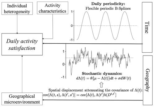
In line with the theoretical framework (Figure 1), the key contribution of this article is to develop a unified spatiotemporal multilevel model with an extended O–U process to simultaneously capture periodicity, stochastic dynamics, and individual heterogeneity effects. Moreover, the developed model benefits and contributes to the SWB studies, providing insights into the complex relationships between geographical microenvironments, situational activity characteristics, and momentary well-being. We further posit that, at the daily activity scale, the specification of correlations between activity satisfaction needs to take into account spatial displacements among activity locations, in addition to the temporal correlation structure implied in the extended O–U process model. The proposal is to attenuate the implied covariance matrix of the stochastic process by spatial distances in line with the well-recognized geographical distance attenuation effect in geography (Tobler 1970; Fotheringham, Brunsdon, and Charlton 2000), as demonstrated in Figure 1. The developed model draws on advances in statistical modeling of intensive longitudinal biomedical data with irregular time intervals among observations (Taylor, Cumberland, and Sy 1994; Diggle, Sousa, and Asar 2015). It also allows, though, for consideration of potential spatial effects among the geo-referenced daily activity observations.

The remainder of this article is structured as follows. The next section describes the proposed space-time modeling framework and estimation strategy. We then provide descriptions on data and variables used in our empirical study, and then present model estimation results in the following sections. The final section concludes the article by discussing research findings and future work.

Developing a Space-Time Modeling Framework for Well-Being

Statistical Model Development

Let i and j index individuals (i = 1, 2, … , n) and activities (j = 1, 2,… , n_i) with n_i being the number of activity episodes conducted by individual i, and t_j the ending time of the jth activity of individual i on a seven-day time axis.¹ For individual i, the developed spatial multilevel O–U process model is expressed as (1) $$Y\left(t_j\right)=X\left(t_j\right)\beta +B\left(t_j\right)+G\left(t_j\right)\delta +\mathrm{\Lambda }\left(t_j\right)+{\varphi }_i+ϵ\left(t_j\right)$$(1) (2) $$\mathrm{d}\mathbf{\Lambda }\left(\mathit{t}\right)=\theta \left\{Z_i^{\prime }\gamma -\mathbf{\Lambda }\left(\mathit{t}\right)\right\}dt+\sigma dW\left(t\right).$$(2)

In these equations, X(t_j) and G(t_j) represent situational activity characteristics and geographical microenvironments of the jth activity performed by individual i, β and δ are two regression coefficient vectors to estimate, and B (·) captures periodicity effects with a B-Spline approach. The scalar-valued random effect ϕ_i measures individual heterogeneity effects on activity satisfaction. It is likely to arise from person-specific biological and personality factors and differs between individuals. Following the convention in the multilevel modeling literature (Raudenbush and Bryk 2002; Goldstein 2011), independent normal distributions are assumed for ϕ_i and ϵ(t_j): ϕ_i ∼ N(0,σ_ϕ²) and ϵ(t_j) ∼ N(0,σ_e²). We note that there is potential for imposing some structured dependence on the individual heterogeneity effects ϕs, for instance, a social network-based correlation structure if such data were available. Given the random sampling strategy adopted in our empirical study, such information is unfortunately not available. Specifying ϕ with a dependence structure shall be an important research avenue, however.

Λ (t) is an extended O–U process for individual i, and W(t) is a stochastic Brownie motion or Wiener process. For t ≥ 0, the increment of W(t) − W(t + Δt) follows a normal distribution, N(0, Δt), and for disjoint time intervals, the corresponding increments of W(t) are independent. It characterizes the stochastic dynamics of daily activity satisfaction and entails two components: The first component induces the mean-reverting property of an O–U process with u_i = Z_i′γ being the equilibrium state and θ (θ > 0) measuring the strength of mean reversion. This mean-reverting property of the O–U process is particularly useful when modeling the trajectory of SWB for an individual. It allows for one person’s SWB to be deviating from the equilibrium level due to the nature of experienced daily activities or events, being it enjoyable, stressful, or anger-provoking. Meanwhile, the model permits a force that pulls back momentary SWB to the equilibrium level such that the variability of one person’s SWB would be bounded rather than being infinite in theory. In addition, the O–U process captures the dynamics or autocorrelations between SWB of successive daily activities in an intuitive way similar to the AR (1) process in the discrete case.²

The second component adds stochastic variability weighted by a variability parameter σ. The random effect ϕ_i could be understood as the unobserved individual characteristics and, together with the observed life-circumstance variables (Z_i), determines the equilibrium state of Λ(t) for individual i. As pointed out in a seminar paper by Sigrist, Künsch, and Stahel (2015), the use of stochastic partial differential equations is not restricted to cases when the true driving force was known a priori, so it is not unreasonable to employ the O–U process to characterize the variability in SWB and make predictions on it. The stationary statistical distribution of the O–U process is a normal distribution with mean Z_i′γ and variance σ²/(2θ), and the covariance matrix of the vector Λ(t) at a stationary state is expressed as (Uhlenbeck and Ornstein 1930; Shreve 2004)³ (3) $$\mathrm{cov}\left({\mathrm{\Lambda }}^i\left(t\right),{\mathrm{\Lambda }}^i\left(s\right)\right)=\frac{{\sigma }^2}{2\theta }{e}^{-\theta |s-t|};\mathrm{ }\left(s,t\right)\in \mathit{t}.$$(3)

To further capture a potential spatiotemporal interaction effect on activity satisfaction, we took a pragmatic approach commonly used in the geostatistics and geographical analysis literature (Cressie 1993; Fotheringham, Brunsdon, and Charlton 2000; Haining 2003); that is, attenuating the previously implied temporal covariance matrix of Λⁱ(t) by geographic distances separating activity sites. This choice was to some extent inspired by our preliminary data analysis. For each resident, we calculated a distance matrix between activity sites, generated a corresponding spatial weights matrix with a Gaussian kernel function, and implemented a spatial lag model (Anselin 1988).⁴ Roughly 82.2 percent (426 out of 518) of estimates on the spatial autoregressive parameter from 518 models were positive and statistically significant at the 95 percent confidence level, with a median of about 0.11 and lower and upper quartiles of (0.08, 0.24). This highlighted the possibility that activities separated by shorter geographical distances tended to be more correlated than those separated by greater distances (Tobler 1970). We, therefore, followed the geographical attenuation effect modeling convention and adjusted the covariance matrix for individual i (Ωⁱ) in the form of (4) $${\mathrm{\Omega }}_{t,s}^i=\mathrm{cov}\left({\mathrm{\Lambda }}^i\left(t\right),{\mathrm{\Lambda }}^i\left(s\right)\right)\times h\left(d_{s,t}\right)=\mathrm{ }\frac{{\sigma }^2}{2\theta }{e}^{-\theta |s-t|}\times e^{-0.5d_{s,t}^2/d_o^2},$$(4) where d_s,t indicates the geographical distance (Euclidean distance) between locations where activities take place at times t and s. This adjustment ensures that the resulting variance–covariance matrix will be positive definite, required by the following model estimation algorithm (Cressie 1993; Banerjee, Carlin, and Gelfand 2014). d_o is a distance threshold or smoothing parameter, with smaller values inducing faster distance attenuation effects in the temporal correlations between activities. In the provided R code files that follow, we also offered the option of using an exponential kernel function. The distance threshold parameter d_o was learned by using an ad-hoc approach (Harris, Dong, and Zhang 2013; G. Dong and Harris 2015; Lu et al. 2023), primarily because it was difficult to distinguish the estimation of the mean-revision parameter θ and d_o (Banerjee, Carlin, and Gelfand 2014). We selected the value of d_o that yielded the largest log-likelihood from a finite discrete set of candidate values from 0.5 km to 10.0 km with a step length of 0.5 km.⁵ An optimal value of 5 km was obtained for d_o. Trivial differences in model estimates were obtained by using other distance threshold parameters such as 4 km or 6 km.

Estimation Algorithm and Implementation

The observations of individual i, Y_i, follow a multivariate normal distribution: ${\mathit{Y}}_{\mathit{i}}\sim \mathit{MVN}({\mathit{\eta }}_{\mathit{i}},{\mathrm{\Sigma }}_i(\mathit{\xi }))$ with ${\mathit{\eta }}_{\mathit{i}}={\tilde{X}}_i\mathit{\varsigma },$ where ${\tilde{X}}_i$ combines the matrices of X(t_j), G(t_j), Z_i′, and the design matrix of B(t_j), and $\mathit{\varsigma }$ are the fixed regression coefficients to be estimated. The unknown parameters $\mathit{\xi }$ in the covariance matrix are [σ_e², σ_ϕ², σ, θ], giving Σ_i = σ_e²I_ni + σ_ϕ²J_ni + Ω_i where I_ni is an identity matrix with dimension of n_i, J_ni an n_i × n_i matrix of ones, and Ω_i being the covariance matrix of the O–U process adjusted by a spatial Gaussian kernel function. Given the assumed independence between individuals, cov (Y_i, Y_k) = 0 for i ≠ k, the log-likelihood function is written as (5) $$\log \hspace{0.17em}L(\mathit{\varsigma },\mathit{\xi })=-\frac{1}{2}\sum _{i=1}^n\log \hspace{0.17em}\left|{\mathrm{\Sigma }}_i\left(\mathit{\xi }\right)\right|+{\left({\mathit{Y}}_{\mathit{i}}-{\tilde{X}}_i\mathit{\varsigma }\right)}^{\prime }{\mathrm{\Sigma }}_i^{-1}\left(\mathit{\xi }\right)\left({\mathit{Y}}_{\mathit{i}}-{\tilde{X}}_i\mathit{\varsigma }\right)+C,$$(5) where C is a constant and |.| denotes the determinant of a square matrix. The maximum likelihood estimators of ($\mathit{\varsigma },$ $\mathit{\xi }$) can be obtained by an iterative Fisher-scoring algorithm (Jennrich and Schluchter 1986; Diggle, Sousa, and Asar 2015). We followed this convention and developed an iterative Fisher-scoring algorithm for model estimation. It proceeded as follows:

1. Updating fixed regression coefficient score vector $\mathit{\varsigma }.$ Denote ${\widehat{\mathit{\varsigma }}}^{(k)}$ and ${\widehat{\mathit{\xi }}}^{(k)}$ as estimates of $\mathit{\varsigma }$ and $\mathit{\xi }$ at the kth scoring step, ${\widehat{\mathit{\varsigma }}}^{(k+1)}$ is updated as (6) $${\widehat{\mathit{\varsigma }}}^{(k+1)}={\left({\sum }_{i=1}^n{\tilde{X}}_i^T{\mathrm{\Sigma }}_i^{-1}\right({\widehat{\mathit{\xi }}}^{\left(k\right)}\left){\tilde{X}}_i\right)}^{-1}\left({\sum }_{i=1}^n{\tilde{X}}_i^T{\mathrm{\Sigma }}_i^{-1}\right({\widehat{\mathit{\xi }}}^{\left(k\right)}\left){\mathit{Y}}_{\mathit{i}}\right).$$(6)

2. Updating parameters in the covariance matrix $\mathit{\xi }.$ ${\widehat{\mathit{\xi }}}^{(k+1)}$ is updated as (7) $${\widehat{\mathit{\xi }}}^{(k+1)}={\widehat{\mathit{\xi }}}^{\left(k\right)}+{\left({\widehat{I}}_{\mathit{\xi }\mathit{\xi }}^{\left(k\right)}\right)}^{-1}{\widehat{\mathit{S}}}_{\mathit{\xi }}\left(k\right)$$(7)

with the score vector ${\widehat{\mathit{S}}}_{\mathit{\xi }}(k)$ calculated as (8) $${{\widehat{\mathit{S}}}_{\mathit{\xi }}\left(k\right)}_{l=1,\dots ,4}=\frac{1}{2}{\sum }_{i=1}^n\mathrm{tr}\left\{{\mathrm{\Sigma }}_i^{-1}\right({\widehat{\mathit{\xi }}}^{\left(k\right)}\left)\right[{\mathbf{r}}_i\left(k+1\right){{\mathbf{r}}_i\left(k+1\right)}^T-{\mathrm{\Sigma }}_i\left({\widehat{\mathit{\xi }}}^{\left(k\right)}\right)\left]{\mathrm{\Sigma }}_i^{-1}\right({\widehat{\mathit{\xi }}}^{\left(k\right)}\left)\frac{\partial {\mathrm{\Sigma }}_i\left(\mathit{\xi }\right)}{\partial {\xi }_l}\right\},$$(8)

where ${\mathbf{r}}_i\left(k+1\right)={\mathit{Y}}_{\mathit{i}}-{\tilde{X}}_i{\widehat{\mathit{\varsigma }}}^{(k+1)}$ and tr (·) is the trace of a square matrix. In the spatial multilevel O–U model, the unknown covariance parameter vector, $\mathit{\xi },$ includes four elements: (σ_e², σ_ϕ², σ, θ). $\partial {\mathrm{\Sigma }}_i\left(\mathit{\xi }\right)/\partial {\xi }_l$ indicate the first-order partial derivatives of the covariance matrix w.r.t each element of $\mathit{\xi }:$ (9) $$\frac{\partial {\mathrm{\Sigma }}_i\left(\mathit{\xi }\right)}{\partial {\sigma }_e^2}=I_{n_i};\mathrm{ }\frac{\partial {\mathrm{\Sigma }}_i\left(\mathit{\xi }\right)}{\partial {\sigma }_{\mathrm{\varnothing }}^2}=J_{n_i};\mathrm{ }\frac{\partial {\mathrm{\Sigma }}_i\left(\mathit{\xi }\right)}{\partial {\sigma }^2}=\frac{1}{2\theta }{e}^{T_i+\frac{1}{2}{D}_i};$$(9) $$\frac{\partial {\mathrm{\Sigma }}_i\left(\mathit{\xi }\right)}{\partial \theta }=-\frac{{\sigma }^2}{2\theta }\left(\frac{1}{\theta }{I}_{n_i}+T_i\right)e^{-\theta T_i+\frac{1}{2}{D}_i},$$ where T_i is a symmetric n_i × n_i paired time difference matrix with elements being |s − t| for s = 1,…,n_i and t = 1,…,n_i. D_i is also a symmetric n_i × n_i matrix with elements being $-0.5d_{s,t}^2/d_o^2$ for s = 1,…, n_i and t = 1,…, n_i. ${\widehat{I}}_{\mathit{\xi }\mathit{\xi }}^{\left(k\right)}$ is the negative expectation of the Hessian matrix of the model log-likelihood, with estimates of $\mathit{\xi }$ at iteration k plugged in, and the (l, m)-th entry is expressed as, (10) $${{\{\widehat{I}}_{\mathit{\xi }\mathit{\xi }}^{\left(k\right)}\}}_{l,m}=\frac{1}{2}{\sum }_{i=1}^n\mathrm{tr}\left\{{\mathrm{\Sigma }}_i^{-1}\left({\widehat{\mathit{\xi }}}^{\left(k\right)}\right)\frac{\partial {\mathrm{\Sigma }}_i\left(\mathit{\xi }\right)}{\partial {\xi }_l}{\mathrm{\Sigma }}_i^{-1}\left({\widehat{\mathit{\xi }}}^{\left(k\right)}\right)\frac{\partial {\mathrm{\Sigma }}_i\left(\mathit{\xi }\right)}{\partial {\xi }_m}\right\}.$$(10)

• III. Convergence and final model parameter estimates. As ${\widehat{I}}_{\mathit{\varsigma }\mathit{\xi }},$ the expectation of second-order cross-derivatives of the log-likelihood function w.r.t fixed regression coefficient vector ζ and covariance parameters ξ, are all equal to 0 (detailed proofs provided in Jennrich and Schluchter 1986), iterating steps (I) and (II) until a convergence condition being met yields the maximum likelihood estimators of model parameters. In the following analysis, the convergence criterion is the squared difference between $\mathit{\xi }(k+1)$ and $\mathit{\xi }(k)$ being less than 10⁻⁷. After samplers achieving convergence (at iteration k^∗), the variance–covariance matrix of $\mathit{\varsigma }$ and $\mathit{\xi }$ is obtained by, (11) $$\mathrm{cov}\left(\widehat{\mathit{\varsigma }}\right)={\left({\sum }_{i=1}^n{\tilde{X}}_i^T{\mathrm{\Sigma }}_i^{-1}\right({\widehat{\mathit{\xi }}}^{\left(k^{\mathrm{*}}\right)}\left){\tilde{X}}_i\right)}^{-1}.$$(11)

Statistical inferences on model parameters can be achieved accordingly. We coded the preceding Fisher-scoring algorithm by using the open-source R language (R Core Team 2017). The code file allows for geographical attenuation effects to be represented by either a Gaussian or an exponential kernel, and for a simpler multilevel O–U model without a consideration of spatial effects. It is useful to note that Fisher scoring is a local optimal algorithm. Model convergence to the selection of initial parameter values should be carefully checked. In this study, a standard multilevel model was implemented first to obtain feasible candidates for the initial values of (σ_e², σ_ϕ²). We then separately fitted model residuals of each respondent with an O–U stochastic differential equation model using the Yuima R package (Iacus and Yoshida 2018), extracted the averages and empirical distributions for parameters (σ, θ), and used them as initial values in our final model implementation. Sensitivity checks were implemented by taking ten random samples from the distributions of (σ_e², σ_ϕ², σ, θ) as different initial values to run the algorithm. The Web link to the code file and a demonstration of its use with simulated data is available at https://osf.io/8h2sr/?view_only=2d81c1d89eff4126af63d43c274c2fb3.

Study Area, Data, and Variables

Our primary data constituted seven days’ GPS trajectories and activity diaries of 709 urban residents, randomly sampled from twenty-three residential communities and nineteen companies in the Shangdi-Qinghe area of Beijing.⁶ Portable GPS receivers (Garmin GPS 60CSx handheld receivers with a Wide Area Augmentation System [WAAS]), recording longitudinal and latitudinal coordinates of locations every five seconds with a positioning accuracy of about 15 m 95 percent of the time, were used to collect participants’ space-time mobility trajectories. At the end of each day during the sampling period, each respondent was asked to fill in a Web-based activity diary with preassigned username and password, wherein she or he can review her or his whole day of mobility trajectories. In the Web diary application, detailed information for each activity conducted by a participant during the day was required to be filled in, including activity types selected from a predefined list of nineteen categories,⁷ companionship, the starting and ending times of an activity, and, importantly, the satisfaction rating of each activity. Another Web questionnaire was developed to collect life-circumstance variables of each participant. Further details of the GPS-based activity-travel survey and sample profiles have been reported elsewhere (Chai et al. 2014).

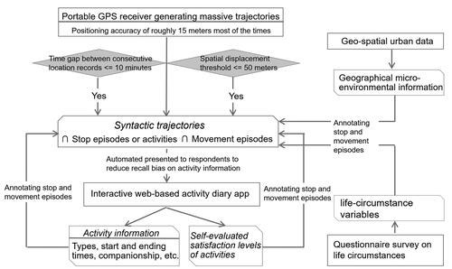
Using a spatial threshold of 50 m and a temporal threshold of ten minutes (adequate time to conduct a meaningful activity), participants’ movement trajectories were characterized as a sequence of consecutive stop and movement episodes (Grinberger and Shoval 2015; G. Dong et al. 2018). These stop episodes of trajectories were then matched to the reported activities and annotated with the attributes of matched activities and life-circumstance variables of corresponding participants. This generated geo-referenced and annotated daily activity data. Only the matched daily activity episodes of participants in the study period were used in our analysis. A flow chart illustrating our data processing procedures and data linkage method is presented in Figure 2. We further excluded participants with incomplete information on some key life-circumstance variables (e.g., income and residence status) and who were full-time students or unemployed, as their daily activity arrangement could differ substantively from that of other groups of people (Shen, Kwan, and Chai 2013). This led to a final data set with 20,557 daily activities from 518 participants analyzed in this study. The original nineteen activity categories were regrouped into eight main activity categories following previous studies (Krizek 2003): working (8.24 percent), leisure (11.70 percent), social (5.97 percent), eating (21.18 percent), family obligation (10.23 percent), grocery shopping (1.13 percent), sleeping (30.16 percent), and others (11.38 percent), with these percentages being the number of recorded activity episodes belonging to each category divided by the total number of activities.

Figure 2. The flow chart showing the key steps and procedures for data processing and linkage.

Similar to the general life satisfaction surveys (Diener, Oishi, and Tay 2018), respondents were asked to report how satisfied they were with each activity (rather than their general life) on a 5-point Likert scale ranging from 1 (very unsatisfied) to 5 (very satisfied). As one of our key empirical contributions to the SWB literature, geographical microenvironments of locations and sites where activities took place were measured and linked to activity satisfaction ratings. In particular, three important dimensions of geographical microenvironment were extracted: ambient air pollution exposure, physical urban form, and urban vibrancy (or liveliness).

Near real-time (hourly) air pollutant concentration (PM_2.5, a particulate matter with diameter of 2.5 µm or less) data from thirty-five monitoring stations in Beijing in the matched periods when the survey was conducted were compiled from Beijing Municipal Environmental Monitoring Center (BMEMC). The Kriging interpolation approach (Yoo et al. 2015) was then used to project hourly PM_2.5 readings from the thirty-five monitoring sites onto a grid layer (with a resolution of 500 m × 500 m) covering Beijing, generating 1,344 hourly pollutant concentration layers in total. Taking advantage of our fine space-time granular daily mobility trajectory data, our measure of air pollution exposure took into account both residents’ daily mobility and the spatiotemporal dynamics of pollutant concentrations, superior to the prevailing static measurement of air pollution exposure at the coarse residential neighborhood scale in previous relevant studies (Park and Kwan 2017; Kwan 2018). As a robustness check on the interpolated pollutant concentration surfaces with the kriging approach, an inverse distance weighted interpolation method was also implemented. The results were quite similar, as evidenced by high Pearson correlation coefficients of interpolated pollutant concentrations from the two approaches with a median of 0.94 and a range of [0.91, 0.98]. We then calculated the activity-wise pollution exposure as a function of activity duration, place of activity, and the dynamics of pollution concentrations: Exposure (k) = ${\int }_{t_0}^{t_1}P(x(t),y(t),t)dt$ where t₀ and t₁ were the starting and ending times of activity k, and P, the PM_2.5 concentration. For practical computation, the integral was approximated by a linear summation of discrete exposures (Lioy 2010).

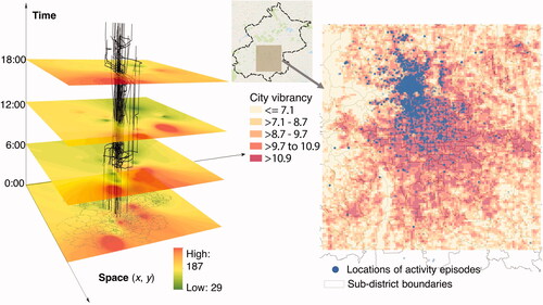
Taking advantage of geospatial urban big data, this article, for the first time, linked urban vibrancy, measuring human activity intensity over space and time or residents’ actual daily use of city spaces (Jacobs 1961), to activity satisfaction, allowing for the conjecture that vibrant places might enhance the experiences of activities to be empirically tested. Mobile phone positioning records, gathered from the most popular Chinese location-based social network services provider Tencent and its mobile phone big data platform Easygo (approximately 450 million records generated by mobile phone users per day in Beijing), were used to infer city vibrancy for each grid cell (as discussed earlier) in Beijing. From the Easygo platform, we compiled mobile phone positioning records per hour per grid over two weeks (15–28 June 2015).⁸ These hourly counts of phone records over two weeks were aggregated to daily counts to reflect day-of-week variability in city vibrancy, with other measures of grid-level vibrancy discussed in the Results section later for robustness checks on our findings. Three-dimensional (space and time) daily trajectories of thirty randomly selected participants are presented in Figure 3, superimposed by time-sliced pollution concentrations and urban vibrancy.

Figure 3. Three-dimensional daily trajectories of thirty randomly selected participants from the research project, with time-sliced ground concentrations of PM_2.5 (left). Geographical locations of selected participants’ daily activities were presented in the right panel of the figure, superimposed by the spatial distributions of urban vibrancy in the study area.

Land-use characteristics of each grid cell in the study area were inferred based on large amounts of geotagged points-of-interest (POI) data, synthesized from online Chinese social media platforms Sina Weibo and Yelp. By calibrating with government land-use data from the Beijing Institute of City Planning, POI-based land-use classification was proved to be accurate and provided higher spatial resolution and detailed categorization (X. Liu and Long 2016). Dominant land-use function of each cell was determined by the dominant POI type in that cell, and the land-use diversity index, measured by the diversity of POI types, was calculated by a widely used entropy measure (X. Liu and Long 2016; Yue et al. 2017): Mix_k =${\sum }_1^J{p}_j\times \ln \hspace{0.17em}{p}_j$ where k is a cell index, j the POI category index, and p_j the proportion of POI type j in cell k.

Activity situational characteristics including activity type, duration, and companionship, and efforts (travel time) made between sequential activities were also included in the model. In addition, life-circumstance variables, including age (mean-centered) and its squared term, income, education qualification, and residence status (migrants vs. local residents), were considered as potential factors of individual equilibrium satisfaction states. The descriptions of variables used in the study are provided in Table 1.

Table 1. Variable description and summaries

Variables	Descriptions	Mean or percentage
Activity satisfaction	Satisfaction ratings on a Likert scale ranging from 1 to 5	3.77 (1.05)
Activity situational variables
Eating	Eating activity	21.2%
Family obligation	Family obligation activities (e.g., family care)	10.2%
Leisure activities	Leisure activities (e.g., gyms, sightseeing)	11.7%
Shopping	Shopping activities	1.1%
Sleeping	Sleeping activities	30.2%
Social activities	Social activities (e.g., social networking)	6.0%
Working	Work/do business	5.2%
Others	Personal care, health care, and so on	14.4%
Duration	The lasting time of an activity (hours)	2.48 (2.55)
With companion	Whether an activity is conducted with a companion	0.382
Weekday	Whether an activity is conducted on weekdays	0.713
Travel time	Travel time between two sequential activities	0.167 (0.46)
Geographical microenvironmental variables
Air pollution	PM2.5 exposure during an activity	140.7 (251.5)
Vibrancy	Population counts of an activity place (1,000)	102.6 (70.8)
Land-use diversity	An entropy-based index of land-use diversity	1.88 (0.31)
Green space	Dominant urban function of sites being green space	3.1%
Residential	Dominant urban function of sites being residential	78.3%
Proximity to main road	Distance of an activity place to urban arterial roads (km)	1.08 (0.86)
Life-circumstance variables
Female	Female participants	52.9%
Age	Age of a participant	34 (8.53)
Monthly income (RMB)
Low	≤ 2,000	11.8%
Medium-low	2,000–4,000	42.1%
Medium	4,000–6,000	23.6%
Medium-high	6,000–10,000	15.4%
High	>10,000	7.1%
With degree	Tertiary educational qualification	58.6%
Married	Married person	74.3%
Migrants	Participants without local household registration	30.2%

Note: RMB = renminbi, official Chinese currency. Standard deviations were also presented for continuous variables.

Results

Descriptive Analysis of Daily Activity Satisfaction

Activity satisfaction, measured on a five-point Likert scale ranging from 1 (very dissatisfied) to 5 (very satisfied), recorded an average of 3.8 with a standard deviation of 1.05. Mapping data onto a seven-day time axis showed a clear one-day cycle (or a twenty-four-hour periodicity) in momentary well-being, a result that was confirmed by a primary periodicity of about twenty-four hours identified from spectral analysis (Larsen 1987). A B-spline polynomial curve with a twenty-four-hour periodicity fitted the aggregated data well with an adjusted R² of 0.63 (Figure 4A). Diurnal rhythm within a day appeared to be stochastic—bouncing back and forth around an overall average after detrending the periodicity—which remained similar across days. Great variability in satisfaction was found across different activity types (Figure 4B): Sleeping, on average, was the least satisfying activity type, followed by daily maintenance activities such as grocery shopping and family obligations, and then working; social and leisure activities were perceived as the most enjoyable activity types. These results are broadly in line with previous findings (Kahneman et al. 2004). The caterpillar plot (Figure 4C) gives proof to the concept that equilibrium states of well-being, measured by averaged satisfaction over seven days after adjusting for activity type effects and periodicity (Headey, Muffels, and Wagner 2010; Diener, Oishi, and Tay 2018), might vary across subpopulations.⁹ For instance, at most income bands local residents and migrants tend to have significantly different equilibrium states, as evidenced by the not much overlapped 95 percent confidence intervals.

Figure 4. Some stylized facts of momentary activity satisfaction learned from data. (A) Mean activity satisfaction over a seven-day time axis was aggregated by using an interval of thirty minutes. Ending times of daily activities were used in the aggregation and the following analyses. The B-Spline curve used was a piece-wise polynomial function of degree 3 in time with internal breakpoints (or knots) being [8, 12, 16, 20] for each calendar day over the seven days (Wood 2017). (B) Bar chart of mean-centered satisfaction of eight types of daily activities with the 95 percent confidence intervals superimposed. (C) A proof of concept that individuals with different life-circumstance variables could be associated with different equilibrium states of well-being. Participants’ monthly income on the x-axis was categorized into five bands: low, median-low, median, median-high, and high. The y-axis is the adjusted satisfaction, which was measured by residuals from a model regressing satisfaction against activity types and the design matrix of a periodic B-Spline polynomial function. (D) Relationships between city vibrancy of activity sites and adjusted satisfaction scores distinguished between activities conducted at home and nonhome locations. (E) Relationships between pollution exposure and adjusted satisfaction for activities conducted at home and nonhome locations with the x-axis being decile-means of pollution exposure (on the log scale).

Because variations in both momentary well-being and microenvironments are evident between home and nonhome places (Ma, Rao, et al. 2020), we analyzed whether geographic contextual effects on satisfaction might be different by activity locations. Figure 4D linked city vibrancy and activity satisfaction by distinguishing between those activities conducted at home and nonhome (nonresidential) locations. It showed that for non-home-based activities, the vibrancy of the activity sites tended to be significantly associated with satisfaction in a nonlinear way: Satisfaction increased with higher levels of vibrancy to a turning point, after which it declined in response to further increases of vibrancy. A second-order polynomial regression yielded a good model fit (adjusted R² = 0.18). In contrast, for home-based activities, vibrancy of a participant’s residential neighborhood did not show a clear relationship with activity satisfaction (Figure 4D). Figure 4E linked activity-wise air pollution exposure to satisfaction for home- and non-home-based activities as well. For activities conducted at home, residents’ subjective experiences did not seem to be affected by ambient air pollution exposure (a slightly upward regression line and very poor model fit). Nonetheless, pollution exposure for activities conducted at nonhome locations appeared to be negatively associated with activity satisfaction and the fitted univariate linear regression yielded a good model fit (adjusted R² = 0.1). Although these preliminary results provided insights into our conceptualization of activity satisfaction (Figure 1), they needed to be further verified with more rigorous statistical models to investigate the effects of activity situational characteristics and microenvironmental variables while capturing the potential spatiotemporal dependencies among activities.

Model Comparisons

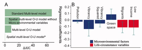
A series of models, from a standard multilevel model without consideration of the stochastic dynamics of activity satisfaction to the developed spatiotemporal multilevel O–U model, were fitted to data. Taking account of spatial displacement between daily activity sites significantly improved model fit, assessed by using the Akaike’s information criterion (AIC, ΔAIC = 9.53 between the spatiotemporal multilevel O–U model with a spatially adjusted O–U process and its counterpart without adjustment for spatial displacement as shown in Figure 5A; Burnham and Anderson 2004). Moreover, removing geographical microenvironmental covariates from the spatiotemporal multilevel O–U model lowered model fit significantly (ΔAIC = 21.41). Together, these two aspects highlighted an added value of embedding geography in the SWB research. As anticipated, the use of a conventional multilevel model resulted in a significant decrease in model fit, thereby highlighting the crucial role of characterizing the stochastic dynamics of daily activity satisfaction (Figure 5A). One important reason is the lack of consideration of the time-dependent correlations between consecutive activities, even conditioning, on the individual-level heterogeneity effect in the classic multilevel models. Besides the relatively poorer performance in terms of model fit from multilevel models, another important consequence would be unreliable statistical inferences on covariate effects.

Figure 5. Model comparison and estimation results. (A) Differences in model fit (ΔAIC) between the spatial multilevel Ornstein–Uhlenbeck (O–U) model (labeled with *) and other models. (B) Covariate effects that were statistically significant at the 5 percent significance level and the associated 95 percent confidence intervals. Presented regression coefficients of ambient air pollution exposure and city vibrancy variables were for activities conducted at nonhome locations, the standard errors of which were calculated by using the delta method.

Model Estimation Results

Table 2 reports the estimation results from the developed spatiotemporal multilevel O–U model, and those from a standard multilevel model as well for comparison. Before proceeding to interpret the covariate effects on activity satisfaction, we highlight two interesting findings in relation to model structure parameters. First, individual-level variability roughly accounted for about 16.6 percent (σ_ϕ^2/(σ_ϕ² + σ_e²)) of the approximate total unexplained variability of activity satisfaction, highlighting the importance of bringing individual differences or heterogeneous effects into the SWB research. Individual heterogeneity includes characteristics of participants that are difficult to measure or observe (e.g., genetics and personality differences), and thus usually unable to be included in statistical models. Our result also corroborates a recent finding that genetic polymorphisms account for as much as 12 to 18 percent of variations in global life satisfaction (Rietveld et al. 2013). Second, the temporal stochastic nature of momentary SWB was also supported, with the estimated mean reversion parameter $\widehat{\theta }$ being about 5.6 (with a standard error of 1.213 and a significance level of 1 percent) and a variability parameter σ² of 0.432.

Table 2. Model estimation results

	Spatial multilevel O–U model		Multilevel model
	Coefficients	SE	Coefficients	SE
Intercept	0.312**	0.097	0.319**	0.096
Activity situational variables
Eating	0.042	0.035	0.044	0.036
Family obligation	–0.02	0.038	–0.02	0.038
Leisure activities	0.079*	0.037	0.08*	0.038
Shopping	–0.004	0.061	–0.004	0.061
Sleeping	–0.846**	0.038	–0.845**	0.036
Social activities	0.051	0.04	0.052	0.036
Others	0.063	0.039	0.063	0.037
Duration	–0.026	0.019	–0.025	0.019
With companion	0.142**	0.016	0.14**	0.016
Weekday	–0.021	0.016	–0.021	0.014
Travel time	–0.002	0.004	–0.002	0.004
Geographical microenvironmental variables
Vibrancy	0.026	0.041	0.025	0.040
Vibrancy squared	0.031	0.022	0.033	0.021
Vibrancy × Non-home	–0.169**	0.063	–0.181**	0.061
Vibrancy squared × Nonhome	–0.088*	0.035	–0.094**	0.034
Air pollution	0.003	0.007	0.002	0.005
Air pollution × Non-home	–0.03**	0.007	–0.031**	0.007
Green space	0.086*	0.042	0.091*	0.041
Residential	0.043	0.031	0.042	0.029
Proximity to main road	0.001	0.005	0.001	0.004
Life-circumstance variables
Migrants	–0.117**	0.043	–0.121**	0.041
Income bands
Low	−0.119*	0.059	−0.121*	0.059
Medium	−0.039	0.045	−0.037	0.046
Medium-high	−0.065	0.057	−0.063	0.057
High	–0.013	0.081	–0.011	0.081
Female	0.015	0.036	0.013	0.036
Age	–0.003	0.003	–0.003	0.003
Age squared	0.001	0.001	0.001	0.001
With degree	0.006	0.040	0.006	0.041
Married	–0.08	0.054	–0.079	0.054
Period effects	Yes		Yes
Covariance parameters ξ
σe^2	0.628	0.007	0.656
θ	5.605	1.793
σϕ^2	0.125	0.01	0.136
σ^2	0.432	0.148
AIC	50822		50889

Note: O–U = Ornstein–Uhlenbeck; AIC = Akaike’s information criterion. Baseline categories for activity type and income bands were working and medium-low, respectively. Period effects were captured by using the B-Splines approach. The standard multilevel model was implemented by using the R package lme4 (Bates et al. 2015).

*p < 0.05.

**p < 0.01.

With respect to situational activity characteristics, statistically significant differences in satisfaction were obtained between activities of different types, and between activities conducted alone or with company. Compared with working activity (the baseline category), sleeping was associated with a much lower level of satisfaction, whereas leisure activities tended to be more enjoyed, everything else being equal. Activities conducted with companions appeared to increase satisfaction by 0.142 standard deviations (p value < 0.001) than those conducted alone. Significant impacts of activity duration and traveling time on satisfaction were not supported, and neither was the weekend effect on satisfaction, a potentially more robust finding than previous studies because of our more credible data, which entailed a complete sequence (rather than snapshots) of residents’ daily activities.

The effects of air pollution exposure on activity satisfaction depended on whether the given activity was conducted at home or at a nonhome location. The difference in effects was statistically significant (the coefficient of the interaction term was −0.03 with a p value < 0.001; Table 2). For home-based activities, ambient air pollution exposure did not appear to exert a statistically significant impact on satisfaction ceteris paribus (Table 2). This was possibly due to the fact that people’s actual indoor pollution exposure at home might be quite different from that in outdoor environments through the use of protective measures such as air purifiers at home. This impact became negative and statistically significant, however, for non-home-based activities (the pollution exposure coefficient was −0.027 with a p value < 0.01 and the 95 percent confidence interval shown in Figure 5B).

As pointed out by Zheng et al. (2019) and Ma, Tao, et al. (2020), residents might modify their trip frequencies and activity arrangements, particularly their nonmandatory social and leisure activities, in response to air pollution levels. Considering that leisure and social activities are typically linked with higher satisfaction levels (Table 2 and Figure 4), if air pollution significantly affects residents’ participation in outdoor leisure and social activities, then the reduced number of more enjoyable activities could partially explain the negative association between air pollution and satisfaction for non-home-based activities. As a robustness check, we implemented a multilevel Poisson regression model, in which the number of nonmandatory social and leisure activities per day was the outcome variable and individual life-circumstance variables and air pollution level (on a log scale) were independent variables. Model estimation results suggested a negative association between air pollution level and the number of nonmandatory activities; that is, higher pollution levels appeared to decrease the number of nonmandatory activities a typical participant would conduct. This association was not statistically significant, however (Table 3), suggesting that our findings on the relationship between air pollution exposure and activity satisfaction were relatively reliable.

Table 3. Estimation results on the impacts of air pollution on the activity arrangement

Variables	Coefficients	Z values
Intercept	0.302*	2.281
Age	–0.002	–0.458
Age squared	0.001	1.446
Female	–0.102*	–1.972
Migrants	–0.163**	–2.640
With degree	–0.038	–0.654
Married	–0.115	–1.495
Income bands
Low	0.037	0.454
Medium	–0.140*	–2.131
Medium-high	–0.176*	–2.116
High	–0.190	–1.609
Air pollution	–0.005	–0.219
Log-likelihood	–4080.8
AIC	8187.5
Individual-level variance	0.166

Note: AIC = Akaike’s information criterion. The multilevel Poisson regression model was implemented by using the R package lme4 (Bates et al. 2015).

*p < 0.05.

**p < 0.01.

Similar to air pollution exposure, the effects of the vibrancy of activity sites on satisfaction varied between home-based and non-home-based activities and the difference was statistically significant (Table 2). For home-based activities, vibrancy (i.e., the residential neighborhood vibrancy) did not appear to affect activity satisfaction (Table 2), whereas both the linear and quadratic terms of vibrancy were statistically significantly associated with activity satisfaction for non-home-based daily activities (regression coefficients for the linear and squared terms were −0.143 and −0.057 with both p values < 0.05 and the calculated 95 percent confidence intervals shown in Figure 5B). These results tended to suggest an inverted-U-shaped relationship between city vibrancy and activity satisfaction, with a turning point roughly equal to the 65th percentile of the distribution of vibrancy in Beijing.

Such an inverted-U-shaped relationship remained under a battery of robustness checks (Table 4). We constructed three different measures of city vibrancy. First, the spatial resolution of the grid topology was degraded to 1 km × 1 km from 500 m × 500 m when building the vibrancy indicator (labeled Measurement 1 in Table 4). Second, the day-of-the week variability of vibrancy over the grid layer was scraped to build a generic spatially varying vibrancy indicator (labeled Measurement 2 in Table 4). Finally, vibrancy was measured by the LandScan Global twenty-four-hour averaged ambient population density data in year 2012, with a resolution of roughly 1 km × 1 km (labeled Measurement 3 in Table 4). Estimation results from these three alternative model specifications are presented in Table 4. The key message was that the preceding findings as to how ambient air pollution exposure and city vibrancy were associated with activity satisfaction were not sensitive to the measurement of city vibrancy. Together, these results highlighted the importance of geographical microenvironments in daily subjective well-being studies, and called for a fine resolution space-time analytical approach to examine subjective well-being variability. The theoretical framework and corresponding empirical statistical modeling approach proposed in this article could serve as a useful starting point.

Table 4. Robustness check results on different city vibrancy measures.

	Measurement 1		Measurement 2		Measurement 3
	Coefficients	Z values	Coefficients	Z values	Coefficients	Z values
Activity situational characteristics
Leisure	0.076*	2.044	0.076*	2.043	0.076*	2.043
Sleeping	–0.849**	–22.220	–0.849**	–22.210	–0.849**	–22.200
With companion	0.142**	8.939	0.141**	8.915	0.140**	8.910
Geographic microenvironmental variables
Vibrancy × Non-home	–0.112**	–2.629	–0.106**	–2.719	–0.098*	–2.325
Vibrancy squared × Nonhome	–0.048*	–2.136	–0.050*	–2.123	–0.041*	–2.037
Pollution × Nonhome	–0.033**	–4.944	–0.032**	–4.741	–0.032**	–4.758
Green space	0.089*	2.098	0.088*	2.101	0.088*	2.186
Life-circumstance variables
Migrants	–0.117**	–2.746	–0.118**	–2.755	–0.118**	–2.743
Income bands
Low	–0.116*	–1.987	–0.117*	–2.002	–0.117*	–2.104
Covariance parameters ξ
σe^2	0.628		0.629		0.629
θ	5.469		5.434		5.437
σϕ^2	0.124		0.124		0.123
σ^2	0.426		0.421		0.423

Note: Model estimation results for vibrancy being measured with a spatial resolution of 1 km × 1 km and without day-of-the-week variability were reported under columns the Measurement 1 and Measurement 2, respectively. Under Measurement 3, vibrancy was measured by the LandScan Global twenty-four-hour averaged ambient population data product in year 2012, with a spatial resolution of roughly 1 km × 1 km. The same set of predictor variables as in the preferred model (Table 2) were included in the two models, but for the sake of saving space, only statistically significant regression coefficients were presented.

*p < 0.05.

**p < 0.01.

In relation to physical urban form variables, land-use diversity of activity site did not appear to affect satisfaction significantly (Table 2). This might be because the direct impact of land-use diversity on activity satisfaction was absorbed by vibrancy, as physical land-use diversity partially contributed to residents’ everyday use of city space (Jacobs 1961; Yue et al. 2017). Activities conducted in sites where green space was the dominant land-use function were significantly associated with higher satisfaction levels than those conducted in sites that possessed other land-use functions (Table 2; MacKerron and Mourato 2013; G. Dong et al. 2016).

Among the individual life-circumstance variables that were suspected to affect individuals’ equilibrium states of well-being, income and residential status were the most significant (Table 2). First, residents in the lowest income band tended to have a much lower equilibrium state of well-being than those who possessed a slightly better economic status (medium-low income), ceteris paribus. Nonetheless, equilibrium state of well-being did not differ statistically significantly between groups in the medium-income band and those with much better economic conditions. This finding is similar to previous studies that have identified a satiating income effect on life satisfaction and emotional well-being (Diener et al. 2010; Jebb et al. 2018). Second, migrants, residents living in the city and contributing to city development but without Beijing household registration (or hukou), were found to have a level of equilibrium well-being state that was about 0.119 standard deviations lower than that of local residents (Table 2). Other life-circumstance variables including age, educational qualifications, and marital status were not statistically significantly associated with equilibrium states of well-being (Table 2). In addition, these results were robust to different measures of urban vibrancy, as illustrated in Table 4.

Discussion and Conclusion

Tracing the trajectories of residents’ daily activities and extracting associated momentary well-being enabled the fine-granular spatiotemporal characteristics of daily SWB to be studied. With space-time referenced daily activity-scale data, geospatial urban big data (from a variety of sources and reflecting many facets of city environment) could be linked, and this opened up great opportunities to investigate how geographical environments shape individuals’ daily activities and associated subjective experiences. This could enable us to go beyond merely answering the question of who is happy versus who is unhappy, and to explore when, and more important, where people are satisfied or unsatisfied with their daily lives. Moreover, incorporating individual daily space-time behaviors and the geographical characteristics of various activity locations into the study of SWB also enables the problem of uncertain geographic contexts to be tackled (Kwan 2012). This is because it enables measurement to be undertaken beyond the relatively coarse-scale residential neighborhood level that tends to be the usual measure of geographical context (Schwanen and Wang 2014). Using only residence-based neighborhoods and ignoring peoples’ exposure to nonresidential contexts could lead to biased estimates of the geographical contextual effects on individuals’ health and well-being (Kwan 2018; Ma, Tao, et al. 2020).

In this study, first and foremost, we presented an integrated space-time analytical framework and developed a corresponding novel statistical model to analyze space-time indexed complex daily activity data, with an explicit treatment of stochastic dynamics, individual heterogeneity, and spatial effects. This method was then applied to explore momentary experiences of daily activities, providing insights into how geographic microenvironments and situational activity characteristics influence individuals’ activity satisfaction. It should be noted that the developed methodology can also be applied to other types of longitudinal data with geospatial information attached and irregularly indexed in the time dimension. These include, for instance, patient tracking data for health analysis and surveillance. Moreover, as a supplement to classic spatiotemporal models dealing with balanced (or regular) data such as variables measured for spatial units over a time period, this methodology is particularly useful for investigating high-resolution space-time data made available by the use of various smart equipment and sensors in urban studies.

Here, we find that daily momentary well-being, besides having a twenty-four-hour periodicity, evolves stochastically around an individual’s equilibrium state that depends on key life-circumstance variables. This strengthens the findings that are usually found in global self-reports about long-term well-being (Diener et al. 2010; Headey, Muffels, and Wagner 2010). The result that migrants have lower equilibrium states of well-being reflects long-standing institutional discrimination against migrants. The hukou system is widely criticized as a tool that blocks social mobility and exacerbates inequalities within and between cities across China. It might be time for the government to seriously consider reforms to the hukou system to improve migrants’ SWB and their long-term integration into the host cities. Further, although geographical microenvironments matter in residents’ subjective experiences of daily activities, their impact differentiates between activities conducted at home and nonresidential locations. Researchers need to be careful to specify the effects of geographical contexts on SWB because of such differences (Schwanen and Wang 2014).

Our finding that air pollution exposure negatively affects subjective experiences of daily activities could offer a microlevel explanation for obtained relationships between air pollution and life satisfaction at individual and areal scales (Ferreira and Moro 2010; Zheng et al. 2019). Such negative SWB impacts of air pollution, observed for residents’ everyday activities, could bring about long-term harms to individuals’ health and work productivity, the so-called hidden effects of air pollution (Zivin and Neidell 2018). It further provides evidence in support of the Chinese government’s clean air initiative from the perspective of improving residents’ daily life experiences, reducing health care costs, and enhancing productivity. High city vibrancy is usually promoted by urban researchers and pursued by city planners and policymakers who seek to use a city’s land efficiently (Jacobs 1961; Yue et al. 2017). Contrary to a simple monotonic relationship, we observed an inverted-U-shaped association between vibrancy and residents’ activity experiences. That is, although at times people might want solitude or intense action, in general they seem to enjoy an intermediate amount of vibrancy. This calls for reflections on the processes and values of Chinese city planning and development policies when seeking to improve individuals’ daily lives as this is an essential component of urban development goals.

Despite this study’s advances, some limitations remain. First, the study employed a spatially adjusted O–U process model to capture both stochastic dynamics and equilibrium states of individual daily activity satisfaction. The selection of this particular stochastic process is underpinned by its mathematical rigor and flexibility, informed by previous literature, and grounded in insights gained from empirical data. One promising research avenue to be pursued in future studies involves the development of innovative stochastic processes that draw inspiration from findings derived from psychological experiments. Furthermore, the space-time interaction in our model was modeled in a pragmatic way, which was intuitive but without a full theoretical treatment of the spatiotemporal processes. Integrating a spatiotemporal advection-diffusion process, formulated with a stochastic partial differential equation (Sigrist, Künsch, and Stahel 2015; Wikle et al. 2022), into a multilevel modeling framework will be able to deal with this limitation. Finally, we shall improve our pragmatic way of modeling potential spatial correlations between activity sites, for instance, by simultaneously modeling the continuous nature of spatial correlation and potential abrupt change effects in space (G. Dong et al. 2020).

Acknowledgments

The authors are grateful for the helpful comments of the reviewers and the editor, which have greatly improved the content of the article. They also much appreciate the insightful comments on the measurement of well-being from Professor Ed Diener at the University of Illinois, who very unfortunately passed away on 27 April 2021. The authors are also grateful to Professor Yanwei Chai from Peking University for allowing us to use the GPS trajectory and activity diary data.

Additional information

Funding

This work was supported by the National Natural Science Foundation of China (Grant Nos. 42001115 and 42071205).

Notes on contributors

Jing Ma

JING MA is an Associate Professor of Human Geography in the Faculty of Geographical Science, Beijing Normal University. E-mail: [email protected] or [email protected]. Her main research interests include activity-travel behavior, subjective well-being, environmental justice, and health.

Guanpeng Dong

GUANPENG DONG is a Professor of Geographic Data Science at the Key Research Institute of Yellow River Civilization and Sustainable Development, Henan University, Kaifeng, China 475001. E-mail: [email protected] and [email protected]. His core research interests include the development of spatial and spatiotemporal statistical and multilevel modeling approaches and their applications in urban studies.

Notes

1 Indexing an activity (an observation here) by using either starting time, ending time, or midpoint time has no influences on model estimation results. Essentially, it is the time gaps between activities that enter our stochastic dynamic process model, and they are the same regardless of activities being indexed by ending or starting time. Also, some key independent variables such as air pollution exposure were constructed based on duration and sites of activities, thus being unaffected by how activities were recorded.

2 With the Euler discretization scheme, most often used for numerically solving deterministic differential equations (Sigrist, Künsch, and Stahel 2015), Equation 2(2) $$\mathrm{d}\mathbf{\Lambda }\left(\mathit{t}\right)=\theta \left\{Z_i^{\prime }\gamma -\mathbf{\Lambda }\left(\mathit{t}\right)\right\}dt+\sigma dW\left(t\right).$$(2) can be reformulated as Λ_t+1 = Λ_t + θ × {Z_i′γ − Λ(t)} Δt + σ × (W_t+1 − W_t). Therefore, Λ_t+1 = ρ × Λ_t + ϵ, where the autocorrelation coefficient ρ = 1 – θ × Δt, and ϵ, the other terms. Such a discrete presentation of the O–U process demonstrates the intuition of modeling temporal autocorrelation and presents a mechanistic explanation. Another advantage of the O–U model lies in its flexibility and capability of dealing with highly complex and irregular time series data structure as discussed in this study.

3 The stationary distribution of the O–U process refers to the time-limiting or the invariant law of the process. The analytical solution to the stochastic partial differential equation can be directly derived by using the Itô lemma (Shreve 2004): ${\mathrm{\Lambda }}_t=\mu +\left({\lambda }_0-\mu \right)e^{-\theta t}+\sigma {\int }_0^t{e}^{-\theta (t-u)}d{W}_u$ where µ = Z′γ in our case. The solution is completely defined by the initial value and an implied Gaussian transition probability distribution, P (Λ_t|Λ₀ = λ₀). As the initial value of a system or process is usually known, and in particular so for an individual’s SWB, we shift our focus, following Wikle et al. (2022), to the stationary distribution of the O–U process.

4 For each individual j, we implemented a spatial lagged dependent model: Y (t_j) = ρ_jWY + B(t_j) + ϵ(t_j), where W was a distance-based spatial weights matrix as discussed in the main text; ρ was the spatial autoregressive parameter, indicating the strength of spatial correlation between activity satisfaction; and B(t_j), a B-Spline function of time, captured possible periodicity effects. To improve estimation efficiency, we have also run a large spatial lag model by stacking individual data and spatial weights matrices together, the estimated ρ was 0.125 with a p value ≤ 0.001.

5 A finite set of distance thresholds were chosen based on the empirical distribution of geographical displacements between daily activities, which ranges from 0 km to 9.85 km.

6 The Shangdi-Qinghe area is located adjacent to the fifth ring road of Beijing on the north, about 16 km away from the city center with a residential population of about 240,000 and an employment population of about 140,000 in 2010 (Ta, Kwan, and Chai 2016). We adopted the multistage clustering sampling approach to randomly select participants from twenty-three residential communities and nineteen corporations in the study area to enhance sampling representativeness. The survey was carried out via eight waves from October to December 2012, and in each wave, 80 to 100 respondents were selected with more than twenty trained investigators involved to provide assistance to the enrolled participants in the seven-day survey (Ta, Kwan, and Chai 2016). In total, 709 participants were enrolled in the project.

7 The predefined nineteen-category list of activities was as follows: 1 = sleeping, 2 = housekeeping, 3 = eating, 4 = shopping, 5 = working, 6 = studying, 7 = strolling, 8 = sports, 9 = picking up and dropping off others, 10 = social activity, 11 = going out for business, 12 = leisure activities, 13 = making telephone calls, 14 = personal care, 15 = taking care of children and the elderly, 16 = surfing the Internet, 17 = seeing the doctor, 18 = tourism, and 19 = others.

8 We acknowledge that the time span of mobile phone data does not overlap with the period when the survey was conducted. A few efforts were made to check the validity of the extracted city vibrancy indicator. We first checked whether the fine-resolution spatial distribution of population was stable or not during 2012 (when our survey was carried out) and 2015 (when the mobile phone positioning records-based measurement of city vibrancy was constructed). The LandScan Global twenty-four-hour averaged ambient population data product with a spatial resolution of roughly 1 km × 1 km in 2012 and 2015, developed by the Oak Ridge National Laboratory (see https://landscan.ornl.gov/), was extracted for the study area, and the Pearson correlation coefficient of the population distribution at the two years was 0.984, indicating a temporally consistent spatial pattern of population distribution. Second, we aggregated our mobile phone data to the same spatial resolution as the LandScan Global population data, and calculated the Pearson correlation coefficients of population density calibrated from the two sources. The resultant correlation coefficient was 0.782, highlighting a good agreement in characterizing population distribution with these two data sources. Finally, LandScan Global population density data in 2012 was used as an alternative variable for measuring city vibrancy. As reported in the following analysis, estimates of model parameters remained stable.

9 To adjust for effects of activity type and periodicity, we first regressed activity satisfaction against activity types and the design matrix of a twenty-four-hour periodic B-Spline polynomial function, and then extracted model residuals as adjusted satisfaction scores.

References

- Ambrey, C., and C. Fleming. 2014. Public greenspace and life satisfaction in urban Australia. Urban Studies 51 (6):1290–1321. doi: 10.1177/0042098013494417.
- Anselin, L. 1988. Spatial econometrics: Methods and models. Dordrecht, The Netherlands: Kluwer Academic.
- Banerjee, S., B. P. Carlin, and A. E. Gelfand. 2014. Hierarchical modeling and analysis for spatial data. Boca Raton, FL: Chapman and Hall/CRC.
- Bates, D., M. Mächler, M. B. Bolker, and S. Walker. 2015. Fitting linear mixed-effects models using lme4. Journal of Statistical Software 67 (1):1–48. doi: 10.18637/jss.v067.i01.
- Birenboim, A. 2018. The influence of urban environments on our subjective momentary experiences. Environment and Planning B: Urban Analytics and City Science 45 (5):915–32. doi: 10.1177/2399808317690149.
- Brereton, F., P. Clinch, and S. Ferreira. 2008. Happiness, geography and the environment. Ecological Economics 65 (2):386–96. doi: 10.1016/j.ecolecon.2007.07.008.
- Brink, M. 2011. Parameters of well-being and subjective health and their relationship with residential traffic noise exposure a representative evaluation in Switzerland. Environment International 37 (4):723–33. doi: 10.1016/j.envint.2011.02.011.
- Burnham, K. P., and D. R. Anderson. 2004. Multimodel inference: Understanding AIC and BIC in model selection. Sociological Methods & Research 33 (2):261–304. doi: 10.1177/0049124104268644.
- Cao, X. J. 2016. How does neighborhood design affect life satisfaction? Evidence from twin cities. Travel Behaviour and Society 5:68–76. doi: 10.1016/j.tbs.2015.07.001.
- Chai, Y., Z. Chen, Y. Liu, N. Ta, and X. Ma. 2014. Space-time behavior survey for smart travel planning in Beijing, China. In Mobile technologies for activity-travel data collection and analysis, 79–90. Hershey, PA: IGI Global.
- Cressie, N. 1993. Statistics for spatial data. New York: Wiley.
- Diener, E., W. Ng, J. Harter, and R. Arora. 2010. Wealth and happiness across the world: Material prosperity predicts life evaluation, whereas psychosocial prosperity predicts positive feeling. Journal of Personality and Social Psychology 99 (1):52–61. doi: 10.1037/a0018066.
- Diener, E., S. Oishi, and L. Tay. 2018. Advances in subjective well-being research. Nature Human Behaviour 2 (4):253–60. doi: 10.1038/s41562-018-0307-6.
- Diggle, P. J., I. Sousa, and O. Asar. 2015. Real-time monitoring of progression towards renal failure in primary care patients. Biostatistics 16 (3):522–36. doi: 10.1093/biostatistics/kxu053.
- Doherty, S. T., C. J. Lemieux, and C. Canally. 2014. Tracking human activity and well-being in natural environments using wearable sensors and experience sampling. Social Science & Medicine 106:83–92. doi: 10.1016/j.socscimed.2014.01.048.
- Dong, G., and R. Harris. 2015. Spatial autoregressive models for geographically hierarchical data structures. Geographical Analysis 47 (2):173–91. doi: 10.1111/gean.12049.
- Dong, G., J. Ma, R. Harris, and G. Pryce. 2016. Spatial random slope multilevel modeling using multivariate conditional autoregressive models: A case study of subjective travel satisfaction in Beijing. Annals of the American Association of Geographers 106 (1):19–35. doi: 10.1080/00045608.2015.1094388.
- Dong, G., J. Ma, M. P. Kwan, Y. Wang, and Y. Chai. 2018. Multi-level temporal autoregressive modelling of daily activity satisfaction using GPS-integrated activity diary data. International Journal of Geographical Information Science 32 (11):2189–2208. doi: 10.1080/13658816.2018.1504219.
- Dong, G., J. Ma, D. Lee, M. Chen, G. Pryce, and Y. Chen. 2020. Developing a locally adaptive spatial multilevel logistic model to analyze ecological effects on health using individual census records. Annals of the American Association of Geographers 110 (3):739–57. doi: 10.1080/24694452.2019.1644990.
- Dong, H., and B. Qin. 2017. Exploring the link between neighborhood environment and mental wellbeing: A case study in Beijing, China. Landscape and Urban Planning 164:71–80. doi: 10.1016/j.landurbplan.2017.04.005.
- Ettema, D., T. Gärling, L. E. Olsson, and M. Friman. 2010. Out-of-home activities, daily travel, and subjective well-being. Transportation Research Part A: Policy and Practice 44 (9):723–32. doi: 10.1016/j.tra.2010.07.005.
- Ettema, D., and M. Schekkerman. 2016. How do spatial characteristics influence well-being and mental health? Comparing the effect of objective and subjective characteristics at different spatial scales. Travel Behaviour and Society 5:56–67. doi: 10.1016/j.tbs.2015.11.001.
- Ferreira, S., and M. Moro. 2010. On the use of subjective well-being data for environmental valuation. Environmental and Resource Economics 46 (3):249–73. doi: 10.1007/s10640-009-9339-8.
- Fotheringham, A. S., C. Brunsdon, and M. Charlton. 2000. Quantitative geography: Perspectives on spatial data analysis. London: Sage.
- Golder, S. A., and M. W. Macy. 2011. Diurnal and seasonal mood vary with work, sleep, and daylength across diverse cultures. Science 333 (6051):1878–81. doi: 10.1126/science.1202775.
- Goldstein, H. 2011. Multilevel statistical models. New York: Wiley.
- Grinberger, A. Y., and N. Shoval. 2015. A temporal-contextual analysis of urban dynamics using location-based data. International Journal of Geographical Information Science 29 (11):1969–87. doi: 10.1080/13658816.2015.1049951.
- Haining, R. 2003. Spatial data analysis: Theory and practice. Cambridge, UK: Cambridge University Press.
- Harris, R., G. Dong, and W. Zhang. 2013. Using contextualized geographically weighted regression to model the spatial heterogeneity of land prices in Beijing, China. Transactions in GIS 17 (6):901–19. doi: 10.1111/tgis.12020.
- Headey, B., R. Muffels, and G. G. Wagner. 2010. Long-running German panel survey shows that personal and economic choices, not just genes, matter for happiness. Proceedings of the National Academy of Sciences of the United States of America 107 (42):17922–26. doi: 10.1073/pnas.1008612107.
- Iacus, S., and N. Yoshida. 2018. Simulation and inference for stochastic process with YUIMA. New York: Springer.
- Jacobs, J. 1961. The death and life of great American cities. New York: Random House.
- Jebb, A. T., L. Tay, E. Diener, and S. Oishi. 2018. Happiness, income satiation and turning points around the world. Nature Human Behaviour 2 (1):33–38. doi: 10.1038/s41562-017-0277-0.
- Jennrich, R., and M. Schluchter. 1986. Unbalanced repeated-measures models with structured covariance matrices. Biometrics 42 (4):805–20. doi: 10.2307/2530695.
- Kahneman, D., A. B. Krueger, D. A. Schkade, N. Schwarz, and A. A. Stone. 2004. A survey method for characterizing daily life experience: The day reconstruction method. Science 306 (5702):1776–80. doi: 10.1126/science.1103572.
- Krizek, K. J. 2003. Neighborhood services, trip purpose, and tour-based travel. Transportation 30 (4):387–410. doi: 10.1023/A:1024768007730.
- Kwan, M. P. 2012. The uncertain geographic context problem. Annals of the Association of American Geographers 102 (5):958–68. doi: 10.1080/00045608.2012.687349.
- Kwan, M. P. 2018. The limits of the neighborhood effect: Contextual uncertainties in geographic, environmental health, and social science research. Annals of the American Association of Geographers 108 (6):1482–90. doi: 10.1080/24694452.2018.1453777.
- Larsen, R. J. 1987. The stability of mood variability: A spectral analytic approach to daily mood assessments. Journal of Personality and Social Psychology 52 (6):1195–1204. doi: 10.1037/0022-3514.52.6.1195.
- Larsen, R. J., and M. Kasimatis. 1990. Individual differences in entrainment of mood to the weekly calendar. Journal of Personality and Social Psychology 58 (1):164–71. doi: 10.1037//0022-3514.58.1.164.
- Leyden, K. M., A. Goldberg, and P. Michelbach. 2011. Understanding the pursuit of happiness in ten major cities. Urban Affairs Review 47 (6):861–88. doi: 10.1177/1078087411403120.
- Lioy, P. J. 2010. Exposure science: A view of the past and milestones for the future. Environmental Health Perspectives 118 (8):1081–90. doi: 10.1289/ehp.0901634.
- Liu, X., and Y. Long. 2016. Automated identification and characterization of parcels with OpenStreetMap and points of interest. Environment and Planning B: Planning and Design 43 (2):341–60. doi: 10.1177/0265813515604767.
- Liu, Y., M. Dijst, and S. Geertman. 2017. The subjective well-being of older adults in Shanghai: The role of residential environment and individual resources. Urban Studies 54 (7):1692–1714. doi: 10.1177/0042098016630512.
- Lu, B., Y. Hu, D. Yang, Y. Liu, L. Liao, Z. Yin, T. Xia, Z. Dong, P. Harris, C. Brunsdon, et al. 2023. GWmodelS: A software for geographically weighted models. SoftwareX 21:101291. doi: 10.1016/j.softx.2022.101291.
- Lucas, R. E. 2007. Adaptation and the set-point model of subjective well-being: Does happiness change after major life events? Current Directions in Psychological Science 16 (2):75–79. doi: 10.1111/j.1467-8721.2007.00479.x.
- Ma, J., G. Dong, Y. Chen, and W. Zhang. 2018. Does satisfactory neighbourhood environment lead to a satisfying life? An investigation of the association between neighbourhood environment and life satisfaction in Beijing. Cities 74:229–39. doi: 10.1016/j.cities.2017.12.008.
- Ma, J., J. Rao, M. P. Kwan, and Y. Chai. 2020. Examining the effects of mobility-based air and noise pollution on activity satisfaction. Transportation Research Part D: Transport and Environment 89:102633. doi: 10.1016/j.trd.2020.102633.
- Ma, J., Y. Tao, M. P. Kwan, and Y. Chai. 2020. Assessing mobility-based real-time air pollution exposure in space and time using smart sensors and GPS trajectories in Beijing. Annals of the American Association of Geographers 110 (2):434–48. doi: 10.1080/24694452.2019.1653752.
- MacKerron, G., and S. Mourato. 2013. Happiness is greater in natural environments. Global Environmental Change 23 (5):992–1000. doi: 10.1016/j.gloenvcha.2013.03.010.
- Morrison, P. S. 2011. Local expressions of subjective well-being: The New Zealand experience. Regional Studies 45 (8):1039–58. –doi: 10.1080/00343401003792476.
- Mouratidis, K., and W. Poortinga. 2020. Built environment, urban vitality and social cohesion: Do vibrant neighborhoods foster strong communities? Landscape and Urban Planning 204:103951. doi: 10.1016/j.landurbplan.2020.103951.
- Nieuwenhuijsen, M. 2016. Urban and transport planning, environmental exposures and health: New concepts, methods and tools to improve health in cities. Environmental Health 15 (Suppl. 1):723– 33. doi: 10.1186/s12940-016-0108-1.
- Park, Y. M., and M. P. Kwan. 2017. Individual exposure estimates may be erroneous when spatiotemporal variability of air pollution and human mobility are ignored. Health & Place 43:85–94. doi: 10.1016/j.healthplace.2016.10.002.
- R Core Team. 2017. R: A language and environment for statistical computing. Vienna, Austria: R Foundation for Statistical Computing.
- Raudenbush, S. W., and A. S. Bryk. 2002. Hierarchical linear models: Applications and data analysis methods. Thousand Oaks, CA: Sage.
- Reis, H. T., K. M. Sheldon, S. L. Gable, J. Roscoe, and R. M. Ryan. 2000. Daily well-being: The role of autonomy, competence, and relatedness. Personality and Social Psychology Bulletin 26 (4):419–35. doi: 10.1177/0146167200266002.
- Rietveld, C. A., D. Cesarini, D. J. Benjamin, P. D. Koellinger, J.-E. De Neve, H. Tiemeier, M. Johannesson, P. K. E. Magnusson, N. L. Pedersen, R. F. Krueger, et al. 2013. Molecular genetics and subjective well-being. Proceedings of the National Academy of Sciences of the United States of America 110 (24):9692–97. doi: 10.1073/pnas.1222171110.
- Schwanen, T., and D. Wang. 2014. Well-being, context, and everyday activities in space and time. Annals of the Association of American Geographers 104 (4):833–51. doi: 10.1080/00045608.2014.912549.
- Shen, Y., M. P. Kwan, and Y. Chai. 2013. Investigating commuting flexibility with GPS data and 3d geovisualization: A case study of Beijing, China. Journal of Transport Geography 32:1–11. doi: 10.1016/j.jtrangeo.2013.07.007.
- Shreve, S. E. 2004. Stochastic calculus for finance II: Continuous-time models. New York: Springer.
- Sigrist, F., H. R. Künsch, and W. A. Stahel. 2015. Stochastic partial differential equation based modelling of large spacetime data sets. Journal of the Royal Statistical Society Series B: Statistical Methodology 77 (1):3–33. doi: 10.1111/rssb.12061.
- Ta, N., M. P. Kwan, and Y. Chai. 2016. Urban form, car ownership and activity space in inner suburbs: A comparison between Beijing (China) and Chicago (United States). Urban Studies 53 (9):1784–1802. doi: 10.1177/0042098015581123.
- Ta, N., H. Li, Y. Chai, and J. Wu. 2021. The impact of green space exposure on satisfaction with active travel trips. Transportation Research Part D: Transport and Environment 99:103022. doi: 10.1016/j.trd.2021.103022.
- Taylor, J. M., W. Cumberland, and J. Sy. 1994. A stochastic model for analysis of longitudinal aids data. Journal of the American Statistical Association 89 (427):727–36. doi: 10.1080/01621459.1994.10476806.
- Tobler, W. R. 1970. A computer movie simulating urban growth in the Detroit region. Economic Geography 46:234–40. doi: 10.2307/143141.
- Tonne, C., C. Mil, D. Fecht, M. Alvarez, J. Gulliver, J. Smith, S. Beevers, R. Anderson, and F. Kelly. 2018. Socioeconomic and ethnic inequalities in exposure to air and noise pollution in London. Environment International 115:170–79. doi: 10.1016/j.envint.2018.03.023.
- Uhlenbeck, G. E., and L. S. Ornstein. 1930. On the theory of the Brownian motion. Physical Review 36 (5):823–41. doi: 10.1103/PhysRev.36.823.
- Welsch, H. 2006. Environment and happiness: Valuation of air pollution using life satisfaction data. Ecological Economics 58 (4):801–13. doi: 10.1016/j.ecolecon.2005.09.006.
- Wikle, N. B., E. M. Hanks, L. Henneman, and C. M. Zigler. 2022. A mechanistic model of annual sulfate concentrations in the United States. Journal of the American Statistical Association 117 (539):1082–93. doi: 10.1080/01621459.2022.2027774.
- Wood, S. N. 2017. Generalized additive models: An introduction with R. Boca Raton, FL: Chapman and Hall/CRC.
- Yoo, E., C. Rudra, M. Glasgow, and L. Mu. 2015. Geospatial estimation of individual exposure to air pollutants: Moving from static monitoring to activity-based dynamic exposure assessment. Annals of the Association of American Geographers 105 (5):915–26. doi: 10.1080/00045608.2015.1054253.
- Yue, Y., Y. Zhuang, A. G. Yeh, J. Xie, C. Ma, and Q. Li. 2017. Measurements of POI based mixed use and their relationships with neighbourhood vibrancy. International Journal of Geographical Information Science 31 (4):658–75. doi: 10.1080/13658816.2016.1220561.
- Zheng, S., J. Wang, C. Sun, X. Zhang, and M. E. Kahn. 2019. Air pollution lowers Chinese urbanites expressed happiness on social media. Nature Human Behaviour 3 (3):237–43. doi: 10.1038/s41562-018-0521-2.
- Zivin, J. G., and M. Neidell. 2018. Air pollution’s hidden impacts. Science 359 (6371):39–40. doi: 10.1126/science.aap7711.