How Mobility and Temporal Contexts May Affect Environmental Exposure Measurements: Using Outdoor Artificial Light at Night (ALAN) and Urban Green Space as Examples

Abstract

Temporal contexts are essential for the derivation of causally relevant environmental exposure in environmental and public health studies. We argue that the proper temporal contexts need further emphasis in the mobility-oriented research paradigm and articulate this issue using a study in Hong Kong. We use people’s exposure to outdoor artificial light at night (ALAN) and green space as two essential examples. We recruited 208 participants from two representative communities in Hong Kong and derived their mobility-oriented environmental exposures from high-resolution remote sensing data and Google Street View imagery. We employed one-standard-deviational ellipses to quantitatively represent participants’ activity spaces, and we further used participants’ seven-day Global Positioning System trajectories to derive their spatiotemporally weighted exposures to green space and outdoor ALAN in different temporal contexts. Multiple t tests were used to examine the disparities in activity spaces and measured exposures in different temporal contexts, and these exposure measurements were then used to predict people’s health outcomes. We found that people’s activity spaces are significantly different in size between day and night, for both weekdays and weekends, and in both geographic contexts. We further observed that improper temporal contexts could lead to significantly different environmental exposure levels and causally irrelevant modeling results.

在环境和公共卫生研究中, 时间背景对于获取环境暴露的因果关系至关重要。我们认为, 流动性研究需要更加强调恰当的时间背景。通过对香港的研究, 我们阐释了这一问题。以人们暴露在户外夜间人造光(ALAN)和绿地为两个重要实例。从两个代表性香港社区招募了208名参与者, 从高分辨率遥感数据和谷歌街景图像中获取了这些参与者们的流动性环境暴露。利用标准偏差椭圆来定量表达参与者的活动空间。根据参与者的七天全球定位系统轨迹, 推导了参与者在不同时间背景下的绿地和户外ALAN时空加权暴露。利用多重t检验来研究不同时间背景下的活动空间和暴露差异, 然后通过这些暴露来预测人们的健康状况。在白天和晚上、工作日和周末以及两种地理环境中, 人们的活动空间大小都有显著差异。我们进一步观察到, 不恰当的时间背景可能导致显著不同的环境暴露水平和无因果关系的建模结果。

Los contextos temporales son esenciales en la derivación de la exposición ambiental causalmente relevante en los estudios ambientales y de salud pública. Sostenemos que los contextos temporales apropiados requieren mayor énfasis en el paradigma investigativo orientado a la movilidad y articulamos este asunto usando un estudio de Hong Kong. Usamos la exposición de la gente a la luz artificial de la calle en la noche (ALAN) y el espacio verde como dos ejemplos esenciales. Reclutamos 208 participantes de dos comunidades representativas de Hong Kong y derivamos sus exposiciones ambientales orientadas a la movilidad a partir de datos de percepción remota de alta resolución e imágenes de Google Street View. Empleamos elipses de una desviación estándar para representar cuantitativamente los espacios de actividad de los participantes, y además usamos las trayectorias de siete días de los participantes, registradas en el Sistema de Posicionamiento Global, para derivar sus exposiciones ponderadas espaciotemporalmente a los espacios verdes y a la ALAN al aire libre, en diferentes contextos temporales. Se utilizaron múltiples pruebas para examinar las disparidades en los espacios de actividad, y las exposiciones medidas en diferentes contextos temporales, y estas medidas de exposición se usaron luego para pronosticar los resultados en la salud de las personas. Encontramos que los espacios de actividad de la gente son significativamente diferentes en tamaño entre el día y la noche, tanto entre semana como en los fines de semana, y en ambos contextos geográficos. Además, observamos que los contextos temporales inadecuados podrían llevar a niveles de exposición ambientales significativamente diferentes, y a resultados de modelización causalmente relevantes.

关键词:

• 夜间人造光(ALAN)
• 测量暴露
• 绿色空间
• 流动性
• 时间背景

Palabras clave:

• contexto temporal
• espacio verde
• luz artificial nocturna (ALAN)
• medición de la exposición
• movilidad

Key Words:

• artificial light at night (ALAN)
• exposure measurement
• green space
• mobility
• temporal context

Advanced geospatial technologies such as Global Positioning Systems (GPS), remote sensing (RS), and geographic information systems (GIS) have fostered the development of the mobility-oriented research paradigm in environmental and public health studies. This novel research paradigm has helped uncover critical knowledge that cannot be acquired through the conventional residence-based research paradigm (Park and Kwan 2017a). Successful studies using mobility-oriented approaches cover people’s exposure to air pollution (Park and Kwan 2017a; Ma et al. 2020), green space (Roberts and Helbich 2021; Lan et al. 2022), noise (El Aarbaoui and Chaix 2020; Tao et al. 2020), traffic congestion (Kim and Kwan 2019; Kan, Kwan, Liu, et al. 2022), and environmental justice (Park and Kwan 2017b; Tao et al. 2021).

The most striking strength of the mobility-oriented research paradigm is its potential for reducing contextual errors arising from ignoring people’s mobility and daily activity contexts (i.e., mitigating the uncertain geographic context problem [UGCoP]; Kwan 2012). Note that conventional approaches (e.g., the time-geographic approach) collect data on people’s mobility using activity-travel diaries (Kwan 2004), which record people’s daily activities and diverse contextual information, including spatiotemporal contexts, activity contexts, and companion contexts. Recent developments in GPS and portable devices with embedded GPS receivers enable the recording of people’s activity-travel trajectories and all visited locations with high temporal resolution and adequate spatial accuracy (K. Lee and Kwan 2018a, 2018b). The new approaches efficiently eliminate recall biases when participants log their diaries. Further, the individual environmental exposure assessment system (IEEAS) developed by Wang et al. (2021) integrates activity-travel diaries, portable GPS devices, mobile sensors, and other instruments to provide the most comprehensive records of people’s real-time contextual information and environmental exposure when people are performing their daily activities and are exposed to various environmental factors.

Contextual information is essential for environmental and public health research, as numerous studies have found that environmental factors might not have the same health effects in different contexts. For example, Ma et al. (2021) observed that transport mode affects people’s microenvironmental exposure and travel satisfaction, and participants tend to report lower satisfaction levels when using enclosed public transport (e.g., bus and subway) and exposed private transport (e.g., walking and cycling) than when using enclosed private transport (e.g., car and taxi). Kou, Kwan, and Chai (2021a, 2021b) found that activity-related contexts significantly influence individuals’ sound evaluations, and surrounding sound is considered more bothersome when participants are working and studying. Kim and Kwan (2021) observed differences between weekdays and weekends in people’s mobility, exposure to ozone, and the manifestation of the neighborhood effect averaging problem.

Temporal context is essential contextual information that has long been overlooked in conventional residence-based epidemiological studies but can be effectively retrieved using the mobility-oriented research paradigm. The first aspect of temporal context stems from the differences between day and night, and people’s exposure to certain environmental factors might be influential during only the daytime or the nighttime. For example, numerous studies have indicated that people’s exposure to artificial light at night (ALAN) is associated with various health risks such as breast cancer (Stevens 2009; Xiao et al. 2020) and depression (Obayashi et al. 2013; Min and Min 2018). Exposure to artificial light should be considered only during nighttime and daytime light exposure should be excluded, however, as daytime light might not disturb human circadian rhythms (Y. Liu, Yu, et al. 2023). Correspondingly, the relevant delineation of people’s activity space should be confined to nighttime activities because the full-day activity space might introduce considerable contextual errors when measuring ALAN exposure. People’s exposure to green space shares a similar mechanism. Because green space might be hardly visible during the night when there is no adequate illumination, it seems unrealistic to assume that the benefits of urban green space to human mental health are the same between days and nights (Figure 1). Correspondingly, the relevant delineation of people’s activity space can be confined to the daytime when measuring people’s exposure to green space. The second aspect of temporal context stems from the mobility difference between weekdays and weekend days. Restrained by work or not, people’s activity space might be drastically different between weekdays and weekend days, whereby people’s exposure to environmental factors could also be drastically different and they may not equivalently affect human health. These two aspects of temporal context are essential for the proper delineation of causally relevant environmental exposure, but relevant studies are very limited to date.

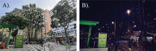
Figure 1. An illustration of the difference in daytime and nighttime exposure to green space. These two pictures were taken from Tai Ming Lane Square in Tai Po, Hong Kong. This green space is enclosed by densely populated communities and intensively used by residents. The greenness of green space during (A) daytime is not visible during (B) nighttime, whereby we cannot assume equivalent effects from green space on human mental health. Other day–night differences in people’s exposure to green space might also affect other health outcomes.

To fill this research gap, we use survey data collected in Hong Kong to conduct a cross-sectional study. We employed people’s exposure to outdoor ALAN as an obvious example and people’s exposure to green space as a less obvious but essential example to discuss the importance of temporal contexts when measuring people’s exposure to environmental factors. Our study seeks to examine (1) whether people’s activity space is significantly different between different temporal contexts in urban areas, (2) whether improper delineation of temporal context will lead to inaccurate assessments of exposure to environmental factors in urban areas, and (3) exposure measurements in which temporal contexts might be causally relevant to people’s health outcomes.

Theoretical Foundation and Analytical Framework for Deriving Contextual Errors Using the Mobility-Oriented Method

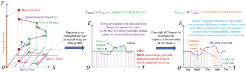
In this analytical section, we first articulate how to derive the contextual error term in the conventional residence-based research paradigm using the mobility-oriented framework, and then extend the derivation to the temporal context error term (Figure 2). We then discuss how the error term is associated with people’s mobility, how it might vary between weekdays and weekends, and how it might affect the modeling of people’s health outcomes.

Figure 2. An illustration of the removal of spatial context errors and temporal context errors using the mobility-oriented research paradigm and temporal constraints. MOM = mobility-oriented measurement; RBM = residence-based measurement.

We first define a person’s environmental exposure E as a function of space s and time t (i.e., E(s, t)). Note that the exposure is measured along a person’s activity-travel trajectories, whereby s is also a function of t (i.e., s(t)) as a person might visit a different place at a different moment. To be concise in the analytics, however, we only denote the symbol of s instead of s(t) to make the equations shorter. Then, people’s accumulated total exposure is an integral of E(s, t) along his or her activity-travel trajectory: (1) $$E_{\mathit{\text{total}}}=\int E\left(s,t\right)\mathit{\text{dt}}.$$(1)

To eliminate the effect of different measurement durations and to have comparable measurements, we revise Equation 1(1) $$E_{\mathit{\text{total}}}=\int E\left(s,t\right)\mathit{\text{dt}}.$$(1) as a spatiotemporally weighted measurement: (2) $$E_{\mathit{\text{total}}}=\frac{\int E\left(s,t\right)\mathit{\text{dt}}}{\int \mathit{\text{dt}}}.$$(2)

For conventional residence-based studies, a person’s exposure to an environmental factor is represented by a constant environmental condition $E_o$ around his or her home location or in a well-defined administrative area. In whichever one, $E(s,t)\equiv E_o,$ and we have: (3) $$E_{\mathit{\text{total}}}=\frac{\int E\left(s,t\right)\mathit{\text{dt}}}{\int \mathit{\text{dt}}}=\frac{\int E_o\mathit{\text{dt}}}{\int \mathit{\text{dt}}}=\frac{E_o\int \mathit{\text{dt}}}{\int \mathit{\text{dt}}}=E_o.$$(3)

In a changing dynamic environment where we have $E\left(s,t\right)=E_o(t),$ we can have a similar derivation: (4) $$E_{\mathit{\text{total}}}=\frac{\int E\left(s,t\right)\mathit{\text{dt}}}{\int \mathit{\text{dt}}}=\frac{\int E_o\left(t\right)\mathit{\text{dt}}}{\int \mathit{\text{dt}}}=\overline{E_o},$$(4) and $\overline{E_o}$ might tend to be temporally constant when we have an adequately long measuring period because the high momentary exposure will always counteract the low momentary exposure. In both Equations 3(3) $$E_{\mathit{\text{total}}}=\frac{\int E\left(s,t\right)\mathit{\text{dt}}}{\int \mathit{\text{dt}}}=\frac{\int E_o\mathit{\text{dt}}}{\int \mathit{\text{dt}}}=\frac{E_o\int \mathit{\text{dt}}}{\int \mathit{\text{dt}}}=E_o.$$(3) and 4(4) $$E_{\mathit{\text{total}}}=\frac{\int E\left(s,t\right)\mathit{\text{dt}}}{\int \mathit{\text{dt}}}=\frac{\int E_o\left(t\right)\mathit{\text{dt}}}{\int \mathit{\text{dt}}}=\overline{E_o},$$(4) , it is clear that the measured exposure from a residence-based approach can be represented by a temporal constant, and ignoring the temporal contexts (e.g., the phase and duration of the measurements) will not lead to a different value of measured exposure only if we have a long enough measuring period and adequate samples. This phenomenon might be the reason why the conventional residence-based approaches by nature would like to overlook the temporal contexts.

The mobility turn in environmental and public health studies argues that a person’s exposure to an environmental factor could significantly change when he or she moves around, whereby the assumption in conventional residence-based approaches that $E(s,t)\equiv E_o$ is not valid and the temporal change might not be periodic. In this case, we can revise Equation 2(2) $$E_{\mathit{\text{total}}}=\frac{\int E\left(s,t\right)\mathit{\text{dt}}}{\int \mathit{\text{dt}}}.$$(2) as follows: (5) $$\begin{array}{c}{E}_{\mathit{\text{total}}}=\frac{\int E\left(s,t\right)\mathit{\text{dt}}}{\int \mathit{\text{dt}}}=\frac{\int E_o-\left[E_o-E\left(s,t\right)\right]\mathit{\text{dt}}}{\int \mathit{\text{dt}}}\\ =\frac{\int E_o\mathit{\text{dt}}}{\int \mathit{\text{dt}}}-\frac{\int E_o-E\left(s,t\right)\mathit{\text{dt}}}{\int \mathit{\text{dt}}}\\ =\frac{E_o\int \mathit{\text{dt}}}{\int \mathit{\text{dt}}}-\frac{\int E_o-E\left(s,t\right)\mathit{\text{dt}}}{\int \mathit{\text{dt}}}=E_o-\frac{\int E_o-E\left(s,t\right)\mathit{\text{dt}}}{\int \mathit{\text{dt}}}.\end{array}.$$(5)

We generally call the term $\frac{\int E_o-E\left(s,t\right)\mathit{\text{dt}}}{\int \mathit{\text{dt}}}$ contextual errors. Due to the existence of contextual errors, residence-based approaches and mobility-oriented approaches are essentially different research paradigms. Numerous empirical studies have indicated that $\frac{\int E_o-E\left(s,t\right)\mathit{\text{dt}}}{\int \mathit{\text{dt}}}$ might be significantly different from 0 and residence-based approaches could lead to erroneous conclusions due to the effects of contextual errors. For example, Y. Liu, Kwan, and Yu (2023) observed multiple significant disparities between residence-based measurements and mobility-oriented measurements of people’s exposure to green space using a range of contextual settings, and these disparities are caused by this contextual error term.

Most recent studies that seek to mitigate contextual errors focus on environmental factors that continuously change with smooth temporal gradients, like air pollution and noise. For other environmental factors, the temporal contexts manifest largely in day–night differences, such as green space and ALAN, whereas the temporal changes in these environmental factors during only the day or only the night can be ignored. For example, people might see exactly the same green space at 10:00 a.m. and 4:00 p.m., but the visible green space at 4:00 p.m. might not be visible or might have drastically different visual quality at 10:00 p.m. if there is no adequate illumination. In this particular case, we can simplify the measurement of exposure as: (6) $$E_{\mathit{\text{total}}}=\frac{\int E\left(s,t\right)\mathit{\text{dt}}}{\int \mathit{\text{dt}}}=\frac{{\int }_{{\mathrm{\Omega }}_d}^{\mathrm{ }}{E}_d\left(s\right)\mathit{\text{dt}}}{{\int }_{{\mathrm{\Omega }}_d}^{\mathrm{ }}\mathit{\text{dt}}}+\frac{{\int }_{{\mathrm{\Omega }}_n}^{\mathrm{ }}{E}_n\left(s\right)\mathit{\text{dt}}}{{\int }_{{\mathrm{\Omega }}_n}^{\mathrm{ }}\mathit{\text{dt}}},$$(6) where $E_d(s)$ is the daytime environmental conditions, $E_n(s)$ is the nighttime environmental conditions, and $E_d\left(s_0\right)\ne E_n\left(s_0\right)$ for any visited place $s_0.$ ${\mathrm{\Omega }}_d$ confines the integral to only the daytime and ${\mathrm{\Omega }}_n$ confines the integral to only the nighttime. Note that s is short for s(t).

A common issue in current studies is ignoring day–night differences and using people’s full-day activity space to derive the accumulated total exposure $E_{\mathit{\text{total}}}.$ Here, we use a person’s exposure to green space as an example. People’s exposure to urban green space could promote their mental health. Visible green space during the daytime might be hardly visible during the nighttime, however. In this case, the day–night difference can be defined as $E_d\left(s\right)\ge 0$ and $E_n(s)\approx 0$ for urban green space’s visibility (Figure 1 as an example). Consequentially, similar to the derivation in Equation 5(5) $$\begin{array}{c}{E}_{\mathit{\text{total}}}=\frac{\int E\left(s,t\right)\mathit{\text{dt}}}{\int \mathit{\text{dt}}}=\frac{\int E_o-\left[E_o-E\left(s,t\right)\right]\mathit{\text{dt}}}{\int \mathit{\text{dt}}}\\ =\frac{\int E_o\mathit{\text{dt}}}{\int \mathit{\text{dt}}}-\frac{\int E_o-E\left(s,t\right)\mathit{\text{dt}}}{\int \mathit{\text{dt}}}\\ =\frac{E_o\int \mathit{\text{dt}}}{\int \mathit{\text{dt}}}-\frac{\int E_o-E\left(s,t\right)\mathit{\text{dt}}}{\int \mathit{\text{dt}}}=E_o-\frac{\int E_o-E\left(s,t\right)\mathit{\text{dt}}}{\int \mathit{\text{dt}}}.\end{array}.$$(5) , we can have: (7) $$\begin{array}{c}{E}_{\mathit{\text{total}}}=\frac{\int E\left(s,t\right)\mathit{\text{dt}}}{\int \mathit{\text{dt}}}=\frac{{\int }_{{\mathrm{\Omega }}_d}^{\mathrm{ }}{E}_d\left(s\right)\mathit{\text{dt}}}{{\int }_{{\mathrm{\Omega }}_d}^{\mathrm{ }}\mathit{\text{dt}}}+\frac{{\int }_{{\mathrm{\Omega }}_n}^{\mathrm{ }}{E}_n\left(s\right)\mathit{\text{dt}}}{{\int }_{{\mathrm{\Omega }}_n}^{\mathrm{ }}\mathit{\text{dt}}}\\ =\frac{{\int }_{{\mathrm{\Omega }}_d}^{ }{E}_d\left(s\right)\mathit{\text{dt}}}{{\int }_{{\mathrm{\Omega }}_d}^{ }\mathit{\text{dt}}}+\frac{{\int }_{{\mathrm{\Omega }}_n}^{ }{E}_d\left(s\right)-\left[E_d\left(s\right)-E_n\left(s\right)\right]\mathit{\text{dt}}}{{\int }_{{\mathrm{\Omega }}_n}^{ }\mathit{\text{dt}}}\\ \begin{array}{c}=\left[\frac{{\int }_{{\mathrm{\Omega }}_d}^{ }{E}_d\left(s\right)\mathit{\text{dt}}}{{\int }_{{\mathrm{\Omega }}_d}^{ }\mathit{\text{dt}}}+\frac{{\int }_{{\mathrm{\Omega }}_n}^{ }{E}_d\left(s\right)\mathit{\text{dt}}}{{\int }_{{\mathrm{\Omega }}_n}^{ }\mathit{\text{dt}}}\right]-\frac{{\int }_{{\mathrm{\Omega }}_n}^{ }{E}_d\left(s\right)-E_n\left(s\right)\mathit{\text{dt}}}{{\int }_{{\mathrm{\Omega }}_n}^{ }\mathit{\text{dt}}}\\ =\frac{\int E_d\left(s\right)\mathit{\text{dt}}}{\int \mathit{\text{dt}}}-\frac{{\int }_{{\mathrm{\Omega }}_n}^{ }{E}_d\left(s\right)-E_n\left(s\right)\mathit{\text{dt}}}{{\int }_{{\mathrm{\Omega }}_n}^{ }\mathit{\text{dt}}},\end{array}\end{array}$$(7) where we can call the term $\frac{\int E_d\left(s\right)\mathit{\text{dt}}}{\int \mathit{\text{dt}}}$ the full-day measurements. It uses the full-day activity space and ignores the day–night differences in environmental factors. We can also call the term $\frac{{\int }_{{\mathrm{\Omega }}_n}^{\mathrm{ }}{E}_d\left(s\right)-E_n\left(s\right)\mathit{\text{dt}}}{{\int }_{{\mathrm{\Omega }}_n}^{\mathrm{ }}\mathit{\text{dt}}}$ the temporal context errors and it can similarly lead to misleading results. Also, because $E_n(s)\approx 0$ for urban green space’s visibility, we can further simplify the temporal context errors as $\frac{{\int }_{{\mathrm{\Omega }}_n}^{\mathrm{ }}{E}_d\left(s\right)\mathit{\text{dt}}}{{\int }_{{\mathrm{\Omega }}_n}^{\mathrm{ }}\mathit{\text{dt}}}.$ Then, this term means the misuse of nighttime activity space to delineate nonexisting nighttime exposure to hardly visible green space. To the best of our knowledge, there are no studies on green space’s health effects that specifically address these temporal context errors.

Via a different mechanism, people’s exposure to ALAN by definition happens only during the night and the main pathways are the disturbance of human circadian rhythms and providing bright space for nighttime activities (Y. Liu, Yu, et al. 2023). Correspondingly, assessment of people’s exposure to ALAN should focus only on the nighttime and daytime light exposure should be excluded. In this case, the day–night difference can be defined as $E_d\left(s\right)\equiv 0$ and $E_n\left(s\right)\ge 0$ for ALAN. Consequentially, similar to the derivation in Equation 7(7) $$\begin{array}{c}{E}_{\mathit{\text{total}}}=\frac{\int E\left(s,t\right)\mathit{\text{dt}}}{\int \mathit{\text{dt}}}=\frac{{\int }_{{\mathrm{\Omega }}_d}^{\mathrm{ }}{E}_d\left(s\right)\mathit{\text{dt}}}{{\int }_{{\mathrm{\Omega }}_d}^{\mathrm{ }}\mathit{\text{dt}}}+\frac{{\int }_{{\mathrm{\Omega }}_n}^{\mathrm{ }}{E}_n\left(s\right)\mathit{\text{dt}}}{{\int }_{{\mathrm{\Omega }}_n}^{\mathrm{ }}\mathit{\text{dt}}}\\ =\frac{{\int }_{{\mathrm{\Omega }}_d}^{ }{E}_d\left(s\right)\mathit{\text{dt}}}{{\int }_{{\mathrm{\Omega }}_d}^{ }\mathit{\text{dt}}}+\frac{{\int }_{{\mathrm{\Omega }}_n}^{ }{E}_d\left(s\right)-\left[E_d\left(s\right)-E_n\left(s\right)\right]\mathit{\text{dt}}}{{\int }_{{\mathrm{\Omega }}_n}^{ }\mathit{\text{dt}}}\\ \begin{array}{c}=\left[\frac{{\int }_{{\mathrm{\Omega }}_d}^{ }{E}_d\left(s\right)\mathit{\text{dt}}}{{\int }_{{\mathrm{\Omega }}_d}^{ }\mathit{\text{dt}}}+\frac{{\int }_{{\mathrm{\Omega }}_n}^{ }{E}_d\left(s\right)\mathit{\text{dt}}}{{\int }_{{\mathrm{\Omega }}_n}^{ }\mathit{\text{dt}}}\right]-\frac{{\int }_{{\mathrm{\Omega }}_n}^{ }{E}_d\left(s\right)-E_n\left(s\right)\mathit{\text{dt}}}{{\int }_{{\mathrm{\Omega }}_n}^{ }\mathit{\text{dt}}}\\ =\frac{\int E_d\left(s\right)\mathit{\text{dt}}}{\int \mathit{\text{dt}}}-\frac{{\int }_{{\mathrm{\Omega }}_n}^{ }{E}_d\left(s\right)-E_n\left(s\right)\mathit{\text{dt}}}{{\int }_{{\mathrm{\Omega }}_n}^{ }\mathit{\text{dt}}},\end{array}\end{array}$$(7) , we can have (8) $$\begin{array}{c}{E}_{\mathit{\text{total}}}=\frac{\int E\left(s,t\right)\mathit{\text{dt}}}{\int \mathit{\text{dt}}}=\frac{{\int }_{{\mathrm{\Omega }}_d}^{\mathrm{ }}{E}_d\left(s\right)\mathit{\text{dt}}}{{\int }_{{\mathrm{\Omega }}_d}^{\mathrm{ }}\mathit{\text{dt}}}+\frac{{\int }_{{\mathrm{\Omega }}_n}^{\mathrm{ }}{E}_n\left(s\right)\mathit{\text{dt}}}{{\int }_{{\mathrm{\Omega }}_n}^{\mathrm{ }}\mathit{\text{dt}}}\\ =\frac{{\int }_{{\mathrm{\Omega }}_d}^{ }{E}_n\left(s\right)-\left[E_n\left(s\right)-E_d\left(s\right)\right]\mathit{\text{dt}}}{{\int }_{{\mathrm{\Omega }}_d}^{ }\mathit{\text{dt}}}+\frac{{\int }_{{\mathrm{\Omega }}_n}^{ }{E}_n\left(s\right)\mathit{\text{dt}}}{{\int }_{{\mathrm{\Omega }}_n}^{ }\mathit{\text{dt}}}\\ \begin{array}{c}=\left[\frac{{\int }_{{\mathrm{\Omega }}_d}^{ }{E}_n\left(s\right)\mathit{\text{dt}}}{{\int }_{{\mathrm{\Omega }}_d}^{ }\mathit{\text{dt}}}+\frac{{\int }_{{\mathrm{\Omega }}_n}^{ }{E}_n\left(s\right)\mathit{\text{dt}}}{{\int }_{{\mathrm{\Omega }}_n}^{ }\mathit{\text{dt}}}\right]-\frac{{\int }_{{\mathrm{\Omega }}_d}^{ }{E}_n\left(s\right)-E_d\left(s\right)\mathit{\text{dt}}}{{\int }_{{\mathrm{\Omega }}_d}^{ }\mathit{\text{dt}}}\\ =\frac{\int E_n\left(s\right)\mathit{\text{dt}}}{\int \mathit{\text{dt}}}-\frac{{\int }_{{\mathrm{\Omega }}_d}^{ }{E}_n\left(s\right)-E_d\left(s\right)\mathit{\text{dt}}}{{\int }_{{\mathrm{\Omega }}_d}^{ }\mathit{\text{dt}}},\end{array}\end{array}$$(8) where $\frac{\int E_n\left(s\right)\mathit{\text{dt}}}{\int \mathit{\text{dt}}}$ is the full-day measurements and the temporal context errors manifest as $\frac{{\int }_{{\mathrm{\Omega }}_d}^{\mathrm{ }}{E}_n\left(s\right)-E_d\left(s\right)\mathit{\text{dt}}}{{\int }_{{\mathrm{\Omega }}_d}^{\mathrm{ }}\mathit{\text{dt}}}.$ Also, because $E_d\left(s\right)\equiv 0$ for ALAN, we can simplify the temporal context errors as $\frac{{\int }_{{\mathrm{\Omega }}_d}^{\mathrm{ }}{E}_n\left(s\right)\mathit{\text{dt}}}{{\int }_{{\mathrm{\Omega }}_d}^{\mathrm{ }}\mathit{\text{dt}}}.$ Then, this term means the misuse of daytime activity space (which should be excluded) to delineate the context for the assessment of ALAN exposure. The example of ALAN is easy to understand because ALAN is by definition a nighttime phenomenon (thus, an obvious example). Because mobility-oriented studies on people’s exposure to ALAN are limited, however, no adequate discussion on these temporal context errors is available to date.

The analytical derivation described earlier indicates that improper delineations of activity space and ignoring the day–night differences in some environmental factors could lead to temporal context errors ($\frac{{\int }_{{\mathrm{\Omega }}_d}^{\mathrm{ }}{E}_n\left(s\right)\mathit{\text{dt}}}{{\int }_{{\mathrm{\Omega }}_d}^{\mathrm{ }}\mathit{\text{dt}}}$ for ALAN and $\frac{{\int }_{{\mathrm{\Omega }}_n}^{\mathrm{ }}{E}_d\left(s\right)\mathit{\text{dt}}}{{\int }_{{\mathrm{\Omega }}_n}^{\mathrm{ }}\mathit{\text{dt}}}$ for green space) and inaccurate assessments of people’s exposure to these environmental factors. These temporal context errors might or might not be significantly different from zero in practice, however. To articulate this issue, this study examines the temporal context errors when assessing people’s exposure to outdoor ALAN and urban green space.

The temporal context error terms can only be derived using the mobility-oriented research paradigm because we illustrated in Equations 3(3) $$E_{\mathit{\text{total}}}=\frac{\int E\left(s,t\right)\mathit{\text{dt}}}{\int \mathit{\text{dt}}}=\frac{\int E_o\mathit{\text{dt}}}{\int \mathit{\text{dt}}}=\frac{E_o\int \mathit{\text{dt}}}{\int \mathit{\text{dt}}}=E_o.$$(3) and 4(4) $$E_{\mathit{\text{total}}}=\frac{\int E\left(s,t\right)\mathit{\text{dt}}}{\int \mathit{\text{dt}}}=\frac{\int E_o\left(t\right)\mathit{\text{dt}}}{\int \mathit{\text{dt}}}=\overline{E_o},$$(4) that the residence-based research paradigm by nature neglects temporal contexts. The fundamental mechanism originates from people’s mobility and variable activity space. Furthermore, another notable temporal context is from the difference in people’s mobility between weekdays and weekend days, whereby the temporal context error term should also be discussed on weekdays and weekend days, respectively.

Study Area and Surveyed Population

We selected Hong Kong as the area for our cross-sectional study because it is one of the most urbanized and densely populated cities in the world. According to the Census and Statistics Department of Hong Kong (2023), about 7.5 million people resided in Hong Kong by the middle of 2023, and 100 percent of them are urbanized. The urban residents in Hong Kong live mainly in two types of communities: old towns developed in earlier times and new towns developed since the 1950s. We chose Sham Shui Po (SSP) as a representative old town community and Tin Shui Wai (TSW) as a representative new town community (Figure 3). The residential blocks included in SSP have an area of 5.35 km² and a population of about 300,000 in 2018; and the residential blocks included in TSW have an area of 4.32 km² and also a population of about 300,000 in 2018 (Y. Liu, Kwan, and Kan 2023).

Figure 3. The geographic settings of Sham Shui Po (SSP) and Tin Shui Wai (TSW). (A) The locations and outdoor artificial light at night (ALAN) distribution of SSP and TSW in Hong Kong. The background is draped using SDGSAT-1 imagery. (B) The geographic settings and land covers of TSW (a new town). (C) The geographic settings and land covers of SSP (an old town). The background is draped using PlanetScope imagery in natural color composition (Planet Team 2017).

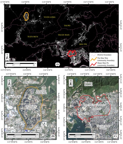
The old towns and new towns represent two different geographic contexts in Hong Kong (Huang and Kwan 2022; Kan, Kwan, Ng, et al. 2022; Y. Liu, Kwan, and Kan 2023), and there are considerable differences between the two geographic contexts regarding building density, urban planning, and traffic networks. SSP represents the old towns and it belongs to the downtown areas of Hong Kong. SSP was developed in the 1920s. The inner city, which is the major part of SSP, has mostly lower, crowded buildings that are directly adjacent to numerous narrow roads. Green space is sparse in SSP but outdoor ALAN is abundant during the night (Figure 3A, 3C). TSW is a typical new town developed in the 1980s in the northwestern part of Hong Kong. The public facilities and infrastructures in TSW are well designed with better open space and the roads are located far from residential buildings with green spaces between them as barriers (Figure 3B). TSW also has abundant outdoor ALAN during the night but is less bright than SSP. The TSW blocks are enclosed by villages and natural parks, they are adjacent to the Hong Kong Wetland Park and Hong Kong’s fish farm regions, and they have slightly more green space than those in SSP.

Data Sets

Questionnaires and GPS-Derived Activity-Travel Trajectories

We recruited 222 participants from SSP and TSW using a stratified sampling method (as a part of a larger project). Written consent for the survey was obtained from each participant, and the data were collected through an integrated IEEAS (Wang et al. 2021). The sociodemographic characteristics of the participants were designed to represent the characteristics of each community regarding residents’ gender, age, marital status, and socioeconomic status. The survey was carried out from 21 March 2021 to 12 September 2021. Each participant was asked to carry a GPS-equipped smartphone continuously for seven days, including five weekdays and two weekend days. The GPS records of each participant were integrated and filtered using the Kalman filter (K. Lee and Kwan 2018a) at the one-minute temporal resolution. The visited locations (in longitude and latitude at each minute) of each participant were sequentially stacked to retrospectively delineate the activity-travel trajectory throughout the whole survey period. Meanwhile, the sociodemographic attributes, self-reported overall health status, and the mental health score of each participant were collected using a questionnaire. The mental health score is surveyed through the commonly used The World Health Organization - Five Well-Being Index (WHO-5) questionnaire (Topp et al. 2015; X. Zhang et al. 2020). Please refer to our previous studies for more details of the survey (Wang et al. 2021; Y. Liu, Kwan, and Kan 2023).

After excluding responses with missing data in the questionnaires and incomplete GPS trajectories, our survey successfully collected valid data from 208 participants, with 104 participants in SSP and the other 104 in TSW. The participants included in our survey cover a range of sociodemographic groups and are representative of the populations in SSP and TSW (Table 1).

Table 1. The sociodemographic profiles and self-reported overall health status in Sham Shui Po (SSP) and Tin Shui Wai (TSW)

Variable		SSP	TSW
Gender	Male	44 (42.3%)	48 (46.2%)
	Female	60 (57.7%)	56 (53.8%)
Age	18–24	16 (15.4%)	21 (20.2%)
	25–44	52 (50.0%)	51 (49.0%)
	45–64	36 (34.6%)	32 (30.8%)
Monthly household income^a	Low	47 (45.2%)	27 (26.0%)
	Middle	32 (30.8%)	48 (46.2%)
	High	25 (24.0%)	29 (27.8%)
Education level^b	Low	37 (35.6%)	36 (34.6%)
	Middle	55 (52.9%)	56 (53.8%)
	High	12 (11.5%)	12 (11.5%)
Marital status^c	Single	53 (51.0%)	58 (55.8%)
	Married	40 (38.5%)	35 (33.7%)
	Others	11 (10.6%)	11 (10.6%)
Overall health status	Excellent/very good/good	91 (87.5%)	93 (89.4%)
	Bad/very bad/terrible	13 (12.5%)	11 (10.6%)
Total		104 (100.0%)	104 (100.0%)

^aMonthly household income: Low-income group has an income of less than 20,000 Hong Kong dollars (HKD), middle-income group has an income of 20,000–39,999 HKD, and the high-income group has an income of 40,000 HKD or above.

^bEducation level: The low group graduated from middle school or lower, the middle group has a bachelor’s degree or certification, and the high group has a master’s degree or higher.

^cOther marital statuses include those divorced and widowed.

Outdoor ALAN in Hong Kong

The outdoor ALAN in Hong Kong is delineated from the SDGSAT-1 Glimmer panchromatic imagery. The cloud-free image was collected from the International Research Center of Big Data for Sustainable Development Goals (http://www.sdgsat.ac.cn/) and it was captured on 12 July 2022. The spatial resolution of the image is 10 m. The image is orthorectified and georeferenced to UTM Zone 49 N coordinate system with reference to the WGS84 ellipsoid. The entire Hong Kong can be covered and the geo-registration reaches a subpixel spatial accuracy. The entire image has no radiometric saturation. The digital numbers (DN) on the image were calibrated to nighttime light luminosity (L) using the following equation (Cui et al. 2023): (9) $$L=\mathit{\text{DN}}\mathrm{*}\mathit{\text{Gain}}+\mathit{\text{Bias}},$$(9) where $\mathit{\text{Gain}}$ and $\mathit{\text{Bias}}$ are the linear calibration coefficients collected from the metadata of the product. The original unit of the luminosity is in $W\bullet m^{-2}\bullet {\mathit{\text{sr}}}^{-1}\bullet {\mu m}^{-1},$ and then converted to $\mathit{\text{nW}}\bullet {\mathit{\text{cm}}}^{-2}\bullet {\mathit{\text{sr}}}^{-1}$ for convenient numbers. Urban outdoor ALAN changes very slowly, especially in well-developed regions like Hong Kong. Consequentially, we assume that our outdoor ALAN imagery can still adequately capture people’s exposure to outdoor ALAN even though the outdoor ALAN imagery is slightly later than our field survey dates.

Google Street View Image Data and the Green View Index in Hong Kong

To comply with our argument on the day–night difference in the visibility of green space and the corresponding impacts on human mental health, we employed Google Street View imagery (SVI) data and corresponding Green View Index (GVI) to derive participants’ exposure to green space. We created a sampling set along Hong Kong’s entire road network in steps of 50 m and collected Google SVI from January to June 2023. At each sampling location, we collected the SVI using the Google Street View Static API (Balali, Rad, and Golparvar-Fard 2015). In total, we set 98,188 sampling points for SVI collection, which can adequately cover the road network of Hong Kong. We further detected the green space area in the field of view in each sampling point using the FCN-8s algorithm (Yao et al. 2019). The GVI is then defined as: (10) $$\mathit{\text{GVI}}=\frac{A\left(\mathit{\text{green space}}\right)}{A\left(\mathit{\text{FOV}}\right)},$$(10) where $\mathit{\text{FOV}}$ is the panoramic field of view in each sampling point and function $A()$ returns the area of either the green space or the entire field of view (Ki and Lee 2021). For our data collection of the Google SVI in Hong Kong, the detection of green space has a producer accuracy of 89.3 percent and a user accuracy of 92.7 percent, and it is adequate for deriving green space exposure using the GVI. The final outcome of the green space derivation is the distribution of the GVI along Hong Kong’s road network, representing the potential daytime greenness in people’s fields of view when traveling. Similarly, urban green space also changes very slowly, especially in well-developed subtropical regions like Hong Kong. Consequentially, we also assume that our GVI data can still adequately capture people’s exposure to green space even though our GVI data are slightly later than our field survey dates.

Methods

The Delineation of People’s Activity Space in Different Temporal Contexts

In this study, we used sunrise and sunset time as criteria to define daytime and nighttime activities because we argued that illumination and human circadian rhythms might be the essential mechanisms to differentiate daytime and nighttime exposure measurements (Wright et al. 2013; Rahm, Sternudd, and Johansson 2021; Zhao, Liu, and Li 2022). Each visited location along each participant’s activity-travel trajectory is coupled with a timestamp at the one-minute temporal resolution. The timestamp is compared with sunrise and sunset time to differentiate daytime and nighttime. If the timestamp of a visited location is after the sunrise time of that day and before the sunset time of that day, the activity in that visited location is designated as a daytime activity; otherwise, the activity in that visited location is designated as a nighttime activity. The sunrise and sunset time are calculated for each visited location of each participant according to the “Astronomy Answers Position of the Sun” (see https://www.aa.quae.nl/en/reken/zonpositie.html, accessed on 10 January 2023). The longitude and latitude of the Hong Kong centroid and the date embedded in each timestamp are used as references to calculate the sunrise and sunset time of that day. An R package called “suncalc” was employed to facilitate the calculation (see https://CRAN.R-project.org/package=suncalc, accessed on 10 January 2023).

The activity-travel trajectories were derived at the one-minute temporal resolution. Missing data exist, however, in the time sequence of visited locations. To mitigate the influence of these missing locations when deriving activity space and estimating exposure, we calculated the temporal weight (${\mathit{\text{WT}}}_i$) of each visited location as follows: (11) $${\mathit{\text{WT}}}_i=\frac{t_{i+1}-t_i}{D},$$(11) where $t_i$ is the timestamp of the ith visited location, $t_{i+1}$ is the next, and $D$ is the total temporal length of the survey period for each temporal context. For example, $D$ has both daytime and nighttime for the full-day measurements, has only the daytime for daytime measurements, and has only the nighttime for nighttime measurements.

We further used the one-standard-deviational ellipse (1-SDE) to represent the activity space of each participant (Woods et al. 2003; Ta et al. 2021). The 1-SDE is derived from the covariance matrix of the coordinates of visited locations while using ${\mathit{\text{WT}}}_i$ as the weight for each visited location. We calculated each participant’s 1-SDE of the visited locations for the entire survey period, weekdays, weekend days, weekday daytime, weekday nighttime, weekend daytime, and weekend nighttime. The size of the 1-SDE is used to represent the size of the participant’s activity space, so a larger area of the 1-SDE indicates a larger activity space of that participant. To increase computational efficiency, a Python script was developed using ArcGIS Pro to implement the procedures.

Estimating People’s Exposure to Outdoor ALAN and Green Space

To comply with the discrete observations in the field surveys and improve the computational efficiency, we discretize the continuous equations in our analytics as spatiotemporally weighted measurements to derive participants’ exposures to outdoor ALAN and green space (L. Zhang et al. 2018; Y. Liu, Kwan, and Yu 2023; Y. Liu, Kwan, Wong, et al. 2023). Through the discretization, the momentary exposure $E\left(s,t\right)$ is considered as the spatial weight ${\mathit{\text{WS}}}_i,$ the temporal differential $\mathit{\text{dt}}$ is replaced by the temporal weight ${\mathit{\text{WT}}}_i,$ and the domain of integral $\mathrm{\Omega }$ is denoted by the phase mark p. The spatiotemporally weighted measurement can yield comparable quantities even though the durations of weekdays and weekend days and daytime and nighttime are not the same. Meanwhile, because our observations have very high temporal resolution, the tiny differences between the continuous approach and the discrete approach can be neglected, and our measurements of exposure can well validate the arguments in our analytics.

Participants’ exposure to green space is calculated as: (12) $$E_{\mathit{\text{GS}}}^P=\frac{\sum {\mathit{\text{WS}}\_\mathit{\text{GS}}}_i^P{\mathit{\text{WT}}}_i^P}{\sum {\mathit{\text{WT}}}_i^P},$$(12) where $E_{\mathit{\text{GS}}}$ is the spatiotemporally weighted exposure to green space along a participant’s activity-travel trajectories; p denotes the phase of interest (temporal context) that includes the entire survey period, weekdays, weekend days, weekday daytime, weekday nighttime, weekend daytime, and weekend nighttime; ${\mathit{\text{WS}}\_\mathit{\text{GS}}}_i$ is the momentary exposure to green space at the ith visited location, which is assigned to the GVI value at the nearest sampling point; and ${ E}_{\mathit{\text{GS}}}$ is a scalar ranging from 0 to 1, where a larger value indicates seeing more green space along a participant’s activity-travel trajectories.

Similarly, participants’ exposure to outdoor ALAN is calculated as: (13) $$E_{\mathit{\text{ALAN}}}^P=\frac{\sum {\mathit{\text{WS}}\_\mathit{\text{ALAN}}}_i^P{\mathit{\text{WT}}}_i^P}{\sum {\mathit{\text{WT}}}_i^P},$$(13) where $E_{\mathit{\text{ALAN}}}$ is the spatiotemporal weighted exposure to outdoor ALAN along a participant’s activity-travel trajectories. ${\mathit{\text{WS}}\_\mathit{\text{ALAN}}}_i$ is the momentary exposure to outdoor ALAN at the ith visited location, which is defined as: (14) $${\mathit{\text{WS}}\_\mathit{\text{ALAN}}}_i=\frac{{\int }_{\mathit{\text{buf}}}^{\mathrm{ }}\mathit{\text{NTL}}\left(x_i,y_i\right)\mathit{\text{da}}}{{\int }_{\mathit{\text{buf}}}^{\mathrm{ }}\mathit{\text{da}}},$$(14) where $\mathit{\text{buf}}$ is the 50-m buffer zone around a participant’s ith visited location $\left(x_i,y_i\right),$ $\mathit{\text{NTL}}$ is the calibrated outdoor ALAN distribution in raster format, and $\mathit{\text{da}}$ is the pixel’s areal size. The 50-m buffer zone is empirically determined because our relevant studies indicate that it could be a causally relevant spatial context. $E_{\mathit{\text{ALAN}}}$ is a scalar no smaller than 0, and a larger value indicates more exposure to outdoor ALAN along a participant’s activity-travel trajectories.

Both exposures to green space and outdoor ALAN were calculated for each participant for the entire survey period, weekdays, weekend days, weekday daytime, weekday nighttime, weekend daytime, and weekend nighttime.

Statistical Analysis

Descriptive analyses were used to examine the distributions of participants’ activity space sizes and exposures to both green space and outdoor ALAN in different temporal contexts. Paired-sample t tests and two-sample t tests were then employed to statistically test the differences in participants’ activity space sizes and exposures to both green space and outdoor ALAN in different temporal contexts.

First, we compared the disparities in participants’ activity space sizes between weekdays and weekends, and between daytime and nighttime. Second, we compared participants’ exposures to outdoor ALAN between the whole survey period and other temporal contexts, including weekdays, weekend days, weekday nighttime, and weekend nighttime. We also compared participants’ exposures to outdoor ALAN between weekdays and weekend days, between weekdays and weekday nighttime, between weekend days and weekend nighttime, and between weekday nighttime and weekend nighttime. The daytime exposures to outdoor ALAN are not considered because they are by definition meaningless. Finally, we compared participants’ exposures to green space between the whole survey period and other temporal contexts. We also compared participants’ exposures to green space between weekdays and weekend days, between weekdays and weekday daytime, between weekend days and weekend daytime, and between weekday daytime and weekend daytime. The nighttime exposures to green space are not considered as the green space is hardly visible during the night and the exposure to them during the night can be ignored in our assumption.

Improper temporal context settings might lead to causally irrelevant exposure measurements when modeling people’s health outcomes. To articulate this issue, we employed binary logistic regression to model participants’ self-reported overall health outcomes using each measured exposure to outdoor ALAN as a predictor, and we also employed quantile regression to model participants’ self-reported mental health outcomes using each measured exposure to green space as a predictor. Several sociodemographic variables are also incorporated into these models to control the effects of possible confounders, including age, gender, educational level, marital status, and socioeconomic status (Su et al. 2019; Y. Liu, Kwan, and Yu 2023). The effect size of the exposure measurement in each temporal context and the corresponding p value are used to discuss their causal relevance.

Results

Disparities in the Size of People’s Activity Space Across Different Temporal Contexts

We first investigated the distributions of participants’ activity space sizes in both SSP and TSW (Table 2 and Figure 4). Note that the original distributions of activity space sizes are heavily skewed, and most distributions have a skewness larger than 2.5. In this study, we took the natural logarithmic values of the original activity space sizes to mitigate the skewness of the original distributions (Table 2). The frequency plots are derived from the natural logarithmic values to more efficiently visualize the shifts in activity space sizes in different temporal contexts (Figure 4). The paired-sample t tests and two-sample t tests were also conducted using the natural logarithmic values of the original activity space sizes to be consistent with the frequency plots (Figure 4).

Figure 4. Disparities in the size of activity space between weekday and weekend, and between daytime and nighttime in (A) Sham Shui Po (SSP) and (B) Tin Shui Wai (TSW). All disparities are significantly different from 0 at the 0.01 level. Small = activity space smaller than –5 in the natural logarithmic value; middle = activity space of 0 in the natural logarithmic value; large = activity space larger than 5 in the natural logarithmic value.

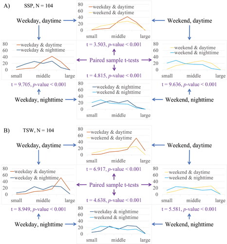
Table 2. Descriptive analyses of participants’ activity space areal size (A) in different temporal contexts

Community	Temporal context	Minimum^a	Median^a	M^a	Maximum^a	SD^a	Skewness	Mean of ln(A)	Skewness of ln(A)
SSP (N = 104)	Weekday daytime	0.01	5.00	15.48	144.29	23.53	2.58	1.48	−0.79
	Weekday nighttime	< 0.01	0.39	4.83	52.61	10.62	3.24	−0.90	−0.56
	Weekend daytime	< 0.01	2.12	17.26	186.40	33.78	2.69	0.46	−0.38
	Weekend nighttime	< 0.01	0.07	2.88	66.95	9.05	5.20	−2.32	−0.13
TSW (N = 104)	Weekday daytime	0.01	31.01	61.30	395.27	85.04	2.18	2.65	−1.08
	Weekday nighttime	< 0.01	2.51	20.87	312.74	43.04	4.04	0.37	−0.58
	Weekend daytime	< 0.01	2.34	16.96	187.35	29.75	2.88	0.31	−0.85
	Weekend nighttime	< 0.01	0.21	12.57	181.48	31.63	3.38	−1.32	−0.25

Note: SSP = Sham Shui Po; TSW = Tin Shui Wai.

^aUnit in km².

Similar to relevant studies, we observed differences between weekday and weekend activity space sizes (Buliung, Roorda, and Remmel 2008; Kamruzzaman and Hine 2012; J. H. Lee et al. 2016). Further, although emphasizing our arguments on the mobility disparities between daytime and nighttime, we have also observed other disparities in activity space sizes. In our study, we observed that participants’ weekday activity spaces are larger than their weekend activity spaces, and their daytime activity spaces are larger than their nighttime activity spaces. All the disparities are significantly different from 0 at the 0.01 level.

The disparities in mobility patterns are similar in different geographic contexts (SSP as an old town and TSW as a new town), but with different magnitudes (Figure 4 and Tables 2 and 3). We observed that participants’ activity space sizes are much larger in TSW than those in SSP during weekday daytime. This difference agrees well with the geographic contexts of the communities. SSP is in the downtown areas whereas TSW is much farther from the downtown areas, and participants in TSW need to commute much longer distances for work than participants in SSP. This difference also manifests in a stronger disparity between weekday daytime and weekend daytime activity space sizes in TSW (t = 6.917; Figure 4B), but a weaker disparity between weekday daytime and weekend daytime activity space areal sizes in SSP (t = 3.503; Figure 4A). In contrast, participants in SSP might commute longer distances than those in TSW for recreational activities during the weekend, which manifests in a stronger disparity between weekend daytime and weekend nighttime activity space sizes in SSP (t = 9.636; Figure 4A), but a weaker disparity between weekend daytime and weekend nighttime activity space sizes in TSW (t = 5.581; Figure 4B).

Table 3. Two-sample t tests of difference in activity space areal sizes between Sham Shui Po (SSP) and Tin Shui Wai (TSW)

Temporal context	t value^a	p value
Weekday daytime	3.808**	< 0.001
Weekday nighttime	2.965**	0.003
Weekend daytime	−0.340	0.734
Weekend nighttime	2.108*	0.036

^aTwo-tailed tests, TSW mean values – SSP mean values, do not assume equal variance.

*Significantly different from each other at the 0.05 level.

**Significantly different from each other at the 0.01 level.

In both SSP and TSW and during both weekdays and weekend days, participants’ nighttime activity space sizes are smaller than their daytime activity space sizes but are not exactly zero. The nighttime activity spaces might originate from commuting home after sunset for some workers with shift work schedules or could be due to some nighttime recreational activities like nighttime running (J. Liu et al. 2020). Because most participants need to use much of their time at night to sleep, it makes sense that their activity space sizes during the nighttime are smaller than those during the daytime. These significant observations then solidly support our argument that the disparities in people’s mobility between different temporal contexts should be taken into account when estimating their exposure to environmental factors, especially using the mobility-oriented research paradigm. In the following sections, we use people’s exposure to outdoor ALAN as an obvious example and people’s exposure to green space as a less obvious example to articulate this issue.

Outdoor ALAN Exposure in Different Temporal Contexts

We first used participants’ exposure to outdoor ALAN as an obvious example to discuss the effects of temporal contexts on environmental exposure measurements. The spatiotemporally weighted approach was employed as it can mitigate the differences from the different durations of different temporal contexts (e.g., weekdays vs. weekend days) and yield comparable measurements. It is long acknowledged that ALAN exposure measurements should be confined to nighttime and thus it is an obvious example. In this section, we further use this obvious example to illustrate how people’s mobility in different temporal contexts might lead to biases in the exposure measurements.

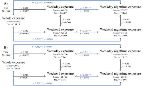
Using the data that we collected, we observed multiple significant disparities in measured exposure to outdoor ALAN in different temporal contexts (Figure 5). All the measured exposures to outdoor ALAN that incorporate irrelevant temporal contexts are different from the accurately measured nighttime exposures to outdoor ALAN. The disparities exist in both SSP and TSW. All the disparities are significantly different from 0 at the 0.01 level.

Figure 5. Differences in measured exposure to outdoor artificial light at night (ALAN) between different temporal contexts in (A) Sham Shui Po (SSP) and (B) Tin Shui Wai (TSW). The unit of measured exposure to outdoor ALAN is in $\mathit{\text{nW}}\bullet {\mathit{\text{cm}}}^{-2}\bullet {\mathit{\text{sr}}}^{-1}.$ **Significantly different from 0 at the 0.01 level.

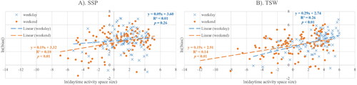
Further, we argue that the error term originates from people’s daytime mobility. We calculated the absolute bias with the following equation: (15) $$\mathit{\text{bias}}=\left|E_{\mathit{\text{ALAN}}}^{\mathit{\text{nighttime}}}-E_{\mathit{\text{ALAN}}}^{\mathit{\text{full day}}}\right|,$$(15) and plot its logarithmic values against the logarithmic values of daytime activity space sizes. In this case, the bias is the isolated temporal context error term $\frac{{\int }_{{\mathrm{\Omega }}_d}^{\mathrm{ }}{E}_n\left(s\right)\mathit{\text{dt}}}{{\int }_{{\mathrm{\Omega }}_d}^{\mathrm{ }}\mathit{\text{dt}}}$ derived from Equation 8(8) $$\begin{array}{c}{E}_{\mathit{\text{total}}}=\frac{\int E\left(s,t\right)\mathit{\text{dt}}}{\int \mathit{\text{dt}}}=\frac{{\int }_{{\mathrm{\Omega }}_d}^{\mathrm{ }}{E}_d\left(s\right)\mathit{\text{dt}}}{{\int }_{{\mathrm{\Omega }}_d}^{\mathrm{ }}\mathit{\text{dt}}}+\frac{{\int }_{{\mathrm{\Omega }}_n}^{\mathrm{ }}{E}_n\left(s\right)\mathit{\text{dt}}}{{\int }_{{\mathrm{\Omega }}_n}^{\mathrm{ }}\mathit{\text{dt}}}\\ =\frac{{\int }_{{\mathrm{\Omega }}_d}^{ }{E}_n\left(s\right)-\left[E_n\left(s\right)-E_d\left(s\right)\right]\mathit{\text{dt}}}{{\int }_{{\mathrm{\Omega }}_d}^{ }\mathit{\text{dt}}}+\frac{{\int }_{{\mathrm{\Omega }}_n}^{ }{E}_n\left(s\right)\mathit{\text{dt}}}{{\int }_{{\mathrm{\Omega }}_n}^{ }\mathit{\text{dt}}}\\ \begin{array}{c}=\left[\frac{{\int }_{{\mathrm{\Omega }}_d}^{ }{E}_n\left(s\right)\mathit{\text{dt}}}{{\int }_{{\mathrm{\Omega }}_d}^{ }\mathit{\text{dt}}}+\frac{{\int }_{{\mathrm{\Omega }}_n}^{ }{E}_n\left(s\right)\mathit{\text{dt}}}{{\int }_{{\mathrm{\Omega }}_n}^{ }\mathit{\text{dt}}}\right]-\frac{{\int }_{{\mathrm{\Omega }}_d}^{ }{E}_n\left(s\right)-E_d\left(s\right)\mathit{\text{dt}}}{{\int }_{{\mathrm{\Omega }}_d}^{ }\mathit{\text{dt}}}\\ =\frac{\int E_n\left(s\right)\mathit{\text{dt}}}{\int \mathit{\text{dt}}}-\frac{{\int }_{{\mathrm{\Omega }}_d}^{ }{E}_n\left(s\right)-E_d\left(s\right)\mathit{\text{dt}}}{{\int }_{{\mathrm{\Omega }}_d}^{ }\mathit{\text{dt}}},\end{array}\end{array}$$(8) . The plots are depicted for both SSP and TSW, and for both weekdays and weekend days (Figure 6). We observed a positive and significant log–log linear relationship (p < 0.01) between temporal context error and daytime activity space size for three cases. In our analytics, we articulated how mobility-oriented measurements can mitigate the contextual errors in residence-based measurements by incorporating people’s mobility and capturing the accurate exposure in real visited locations. We further extended this approach to mitigate the temporal context errors by applying proper temporal contexts. Regarding people’s exposure to outdoor ALAN, the daytime activity space is the source of temporal context errors in the full-day measurements. Correspondingly, a larger daytime activity space might induce more temporal context errors in outdoor ALAN exposure measurements. These plots in Figure 6 clearly indicate that improper temporal contexts (daytime) might significantly lead to biases through people’s mobility and improper activity space. The comparatively small $R^2$ values, however, also indicate that mobility might not be the only factor of biases, and an alternative impact factor might be the uneven distribution of environmental factors. This phenomenon is a typical manifestation of the UGCoP, and it emphasizes that we need to consider human mobility, environmental settings, and temporal contexts to obtain accurate assessments of people’s exposure to environmental factors.

Figure 6. The dot plots of the biases in participants’ exposure to outdoor artificial light at night (ALAN) against their daytime activity space areal sizes in (A) Sham Shui Po (SSP) and (B) Tin Shui Wai (TSW).

Green Space Exposure in Different Temporal Contexts

In the previous section, we discussed how temporal context could affect exposure measurement via human mobility and improper activity space, and we use people’s exposure to outdoor ALAN as an obvious example. In this section, we further argue that this issue might be general for a broad scope of environmental exposure measurements and we use people’s exposure to green space as a second example. The temporal context in measuring people’s exposure to green space has long been overlooked because it is not straightforward, and we call it a less obvious but essential example.

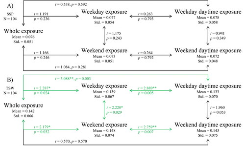
We observed multiple significant disparities in green space exposure in TSW (Figure 7) when using different temporal contexts. The significant disparities of TSW participants’ exposure measurements between weekday and weekday daytime, and between weekend and weekend daytime can be directly attributed to the temporal context error term $\frac{{\int }_{{\mathrm{\Omega }}_n}^{\mathrm{ }}{E}_d\left(s\right)\mathit{\text{dt}}}{{\int }_{{\mathrm{\Omega }}_n}^{\mathrm{ }}\mathit{\text{dt}}}$ discussed in our analytics. This temporal context error term further leads to a significant disparity of TSW participants’ exposure measurements between the whole survey period and weekday daytime, because the whole survey period also contains improper temporal contexts. The temporal context error term, however, might not lead to statistically significant disparities in some cases, such as the case between the whole survey period and weekend daytime in TSW and all the cases in SSP. Note that Hong Kong is a highly urbanized city with a sparse, scattering, and spatially uneven coverage of green space. According to our delineation of Hong Kong green space, SSP has a green space coverage of 13.6 percent, and TSW has coverage of 15.5 percent. That might be the reason why we did not observe significant disparities in SSP.

Figure 7. Differences in measured exposure to green space between different temporal contexts in (A) Sham Shui Po (SSP) and (B) Tin Shui Wai (TSW). Measurement is unitless. *Significantly different from 0 at the 0.05 level. **Significantly different from 0 at the 0.01 level.

Modeling People’s Health Outcomes

In the previous two sections, we illustrated how different temporal contexts could lead to different values of outdoor ALAN and green space exposure measurements, and we argue that these significant disparities are caused by people’s apparent mobility differences in various temporal contexts. In this section, we further articulate that the causally relevant exposure measurements in the proper temporal contexts are also essential for modeling people’s health outcomes (Table 4). The temporal contextual errors could enlarge the uncertainties when estimating the effect sizes of corresponding environmental exposures, resulting in the shift of effect magnitudes, longer error bars, and downgraded significance levels. These inaccurately estimated effects and significance levels might lead to insignificant results and wrong conclusions while the actual associations are significant (i.e., Type II errors; Kwan 2012). In contrast, the proper exposure measurements can considerably reduce the risk of Type II errors after excluding temporal contextual errors, and lead to significant results and correct conclusions. We observed one significant association between TSW participants’ exposure to weekday nighttime outdoor ALAN and their self-reported overall health statuses and one significant association between SSP participants’ exposure to weekday daytime green space and their self-reported mental health scores. These results are well consistent with previous studies (Y. Liu, Kwan, and Yu 2023), and the disparities between SSP and TSW can be attributed to communities’ specific geographic contexts and spatial nonstationarity (Kwan 2021).

Table 4. Model participants’ self-reported overall health and mental health using outdoor artificial light at night (ALAN) and green space exposure in different temporal contexts

Input		SSP (N = 104)			TSW (N = 104)
		Logit^a	SE	p value	Logit^a	SE	p value
Outdoor ALAN exposure	Whole day	0.000	0.001	0.876	0.006	0.004	0.158
	Weekday	0.000	0.001	0.868	0.005	0.004	0.190
	Weekday nighttime	−0.001	0.001	0.396	0.010*	0.005	0.037
	Weekend	0.000	0.001	0.955	0.003	0.003	0.298
	Weekend nighttime	0.001	0.002	0.543	0.006	0.004	0.128
Input		B^a^,^b	SE	p value	B^a^,b	SE	p value
Green space exposure	Whole day	−9.071	7.087	0.204	6.288	5.727	0.275
	Weekday	−8.094	7.108	0.258	6.389	5.688	0.264
	Weekday daytime	−13.862*	5.674	0.017	6.470	5.806	0.268
	Weekend	−8.362	6.552	0.205	4.680	5.385	0.387
	Weekend daytime	−5.548	7.350	0.452	4.205	5.310	0.341

Note: SSP = Sham Shui Po; TSW = Tin Shui Wai.

^aThe estimated logit values in the binary logistic models and the estimated coefficients (B) in the quantile models were adjusted by age, gender, educational level, marital status, and socioeconomic status.

^bThe quantile (q) is set to 50 percent in these quantile models.

*Significantly different from 0 at the 0.05 level. Significant results are highlighted in bold.

It is evident that people’s exposure to outdoor ALAN should be confined to nighttime. We observed that it is easy to have an insignificant Logit when using a wrong temporal context to derive people’s exposure to outdoor ALAN. We also observed that the outdoor ALAN exposure measured on weekend nighttime is not significantly associated with participants’ self-reported health statuses. For most participants, weekend nighttime outdoor ALAN exposure is from leisure activities and it is random and unpredictable. In contrast, weekday nighttime activities and weekday nighttime outdoor ALAN exposure might be more causally relevant because they could contain regular activities such as commuting home at night, whereby we can observe a significant association in TSW (Table 4).

Similarly, we also observed that only the weekday daytime green space exposure measurements have a significant association with SSP participants’ mental health scores. When using improper temporal contexts like the full-day measurements, we cannot observe any significant associations. These observations agree well with our argument that green space might be hardly visible during nighttime and the full-day measurements contain too many green space exposures that do not have impacts on human mental health (i.e., temporal context errors), leading to erroneous conclusions. We did not observe significant associations between green space exposure measurements and SSP participants’ mental health scores during weekend days, whether we used full-day measurements or daytime measurements. This phenomenon might also be attributed to people’s free mobility during leisure activities on weekend days, and these exposure measurements are not representative because the activity-travel trajectories are irregular.

Discussion

In this study, we investigated how people’s mobility and various temporal contexts might affect exposure measurements of environmental factors such as outdoor ALAN and green space. We observed significant differences in people’s activity space sizes between daytime and nighttime, regardless of weekdays or weekend days, and in both geographic contexts of a new town and an old town in Hong Kong. We analytically derived the temporal context error terms using the mobility-oriented research paradigm and successfully isolated the error terms from different exposure measurements in various temporal contexts. We finally illustrated how these temporal context errors could affect the modeling of people’s health outcomes. We also highlighted that the proper temporal contexts can only be retrieved using the mobility-oriented research paradigm, and the residence-based research paradigm by nature would like to overlook the temporal contexts.

Our results have significant methodological implications for environmental and public health studies regarding obtaining accurate assessments of people’s exposure to environmental factors. In recent years, it has become a stronger argument to incorporate people’s mobility and environmental dynamics when measuring their exposure to environmental factors, and the mobility-oriented research paradigm has shown promising advantages over the conventional residence-based research paradigm for minimizing contextual errors and mitigating the UGCoP (Kwan 2012). Our results further emphasize the need to carefully consider time-variant environmental factors or contexts to minimize temporal context errors. The differences between day and night, between weekdays and weekend days, and in people’s mobility should be carefully considered when measuring people’s exposure to various environmental factors.

Our results are also essential manifestations of the nonstationarity in environmental and public health studies (Kwan 2021). The emphasis on temporal contexts is a typical manifestation of temporal nonstationarity. Our results indicate that accurate assessments of people’s exposure to environmental factors rely on careful consideration of the causally relevant temporal contexts. On the other hand, inaccurate exposure assessments might or might not be significantly different from accurate assessments in practice, and they might or might not lead to different conclusions in modeling people’s health outcomes. This is a typical manifestation of spatial nonstationarity and it highly depends on the concrete geographic contexts. Even though we observed significant associations, our results indicate that daytime activity space sizes cannot well explain the biases in the measurements of people’s exposure to outdoor ALAN when ignoring the day–night differences in people’s mobility. Hence, we argue that the inaccurate assessments of people’s exposure to environmental factors cannot be singly and simply attributed to only ignoring the day–night differences in people’s mobility. Using people’s trajectories with a fine spatiotemporal resolution, adopting the models of environmental factors that can spatiotemporally overlap with people’s daily activity-travel trajectories, and estimating the momentary exposure to environmental factors within well-defined spatiotemporal contexts are currently the most promising approaches to mitigating these issues.

We also acknowledge that this study has some limitations. This study is a cross-sectional study with a short survey period. We have discussed the temporal contexts of day and night and weekday and weekend. This data set is not adequate, however, for examining the longer term effects of environmental factors and the temporal nonstationarity of other temporal contexts. Meanwhile, due to the difficulties in data collection, our sample size is comparatively small. Although this data set is adequate to represent the populations in different geographic contexts, it is not adequate for a focus on disadvantaged groups that need more attention. Our future studies will benefit from using a longitudinal approach with a much larger sample size.

Conclusions

We investigated how mobility and temporal contexts could affect exposure measurements of environmental factors. We used people’s exposure to outdoor ALAN as an obvious example and people’s exposure to green space as a less obvious but essential example. The GPS trajectories at the one-minute temporal resolution, the sociodemographic attributes, and the participants’ self-reported health outcomes were collected from 208 participants in two representative communities in Hong Kong. Participants’ exposures to outdoor ALAN and green space were measured using a spatiotemporally weighted approach in different temporal contexts. We observed significant disparities in people’s mobility in different temporal contexts. We then analytically derived the temporal context error terms and empirically illustrated how they lead to exposure measurement biases, associate with people’s mobility, and affect the modeling of people’s health outcomes.

Our results are essential manifestations of multiple methodological issues, including the UGCoP, and spatial and temporal nonstationarity. We argue that temporal contexts should be carefully constrained to acquire accurate measurements of people’s exposure to some environmental factors. This study provides fundamental implications for a broad scope of environmental and public health studies by emphasizing the role of proper temporal constraints in the accurate measurements of environmental exposures.

Acknowledgments

We thank the editor and the reviewers for their helpful comments. In addition, we would also like to express our gratitude to all the participants who generously devoted their time to the study.

Disclosure Statement

No potential conflict of interest was reported by the authors.

Additional information

Funding

This research was supported by grants from the Hong Kong Research Grants Council (General Research Fund Grant Nos. 14605920, 14606922; Collaborative Research Fund Grant No. C4023-20GF; Research Matching Grants RMG 8601219, 8601242), and a grant from the Research Committee on Research Sustainability of Major Research Grants Council Funding Schemes (3133235) of the Chinese University of Hong Kong. The funders had no role in study design, data collection and analysis, decision to publish, or preparation of the manuscript.

Notes on contributors

Yang Liu

YANG LIU is a PhD Candidate in the Department of Geography and Resource Management and the Institute of Space and Earth Information Science at the Chinese University of Hong Kong, Hong Kong Special Administrative Region of China. E-mail: [email protected]. His research interests include urban green space, artificial light at night (ALAN), human mobility, environmental and public health, remote sensing, and GIScience.

Mei-Po Kwan

MEI-PO KWAN is Head of Chung Chi College, Choh-Ming Li Professor of Geography and Resource Management, Director of the Institute of Space and Earth Information Science, and Director of the Institute of Future Cities at the Chinese University of Hong Kong, Hong Kong Special Administrative Region of China. E-mail: [email protected]. Her research interests include environmental health, human mobility, sustainable cities, transport and health issues in cities, and GIScience. She is a leading researcher in deploying real-time GPS tracking and mobile sensing to collect individual-level data in environmental health research.

Changda Yu

CHANGDA YU is a PhD Candidate in the Institute of Space and Earth Information Science at the Chinese University of Hong Kong, Hong Kong Special Administrative Region of China. E-mail: [email protected]. His research interests include environmental health, human mobility, and GIScience.

References

- Balali, V., A. A. Rad, and M. Golparvar-Fard. 2015. Detection, classification, and mapping of US traffic signs using Google Street View images for roadway inventory management. Visualization in Engineering 3 (1):1–18. doi: 10.1186/s40327-015-0027-1.
- Buliung, R. N., M. J. Roorda, and T. K. Remmel. 2008. Exploring spatial variety in patterns of activity-travel behaviour: Initial results from the Toronto Travel-Activity Panel Survey (TTAPS). Transportation 35 (6):697–722. doi: 10.1007/s11116-008-9178-4.
- Census and Statistics Department. 2023. Mid-year population for 2023 [15 Aug 2023]. The Government of the Hong Kong Special Administrative Region. Accessed December 29, 2023. https://www.censtatd.gov.hk/en/press_release_detail.html?id=5265.
- Cui, Z., C. Ma, H. Zhang, Y. Hu, L. Yan, C. Dou, and X.-M. Li. 2023. Vicarious radiometric calibration of the multispectral imager onboard SDGSAT-1 over the Dunhuang calibration site, China. Remote Sensing 15 (10):2578. doi: 10.3390/rs15102578.
- El Aarbaoui, T., and B. Chaix. 2020. The short-term association between exposure to noise and heart rate variability in daily locations and mobility contexts. Journal of Exposure Science & Environmental Epidemiology 30 (2):383–93. doi: 10.1038/s41370-019-0158-x.
- Huang, J., and M.-P. Kwan. 2022. Examining the influence of housing conditions and daily greenspace exposure on people’s perceived COVID-19 risk and distress. International Journal of Environmental Research and Public Health 19 (14):8876. doi: 10.3390/ijerph19148876.
- Kamruzzaman, M., and J. Hine. 2012. Analysis of rural activity spaces and transport disadvantage using a multi-method approach. Transport Policy 19 (1):105–20. doi: 10.1016/j.tranpol.2011.09.007.
- Kan, Z., M.-P. Kwan, D. Liu, L. Tang, Y. Chen, and M. Fang. 2022. Assessing individual activity-related exposures to traffic congestion using GPS trajectory data. Journal of Transport Geography 98:103240. doi: 10.1016/j.jtrangeo.2021.103240.
- Kan, Z., M.-P. Kwan, M. K. Ng, and H. Tieben. 2022. The impacts of housing characteristics and built-environment features on mental health. International Journal of Environmental Research and Public Health 19 (9):5143. doi: 10.3390/ijerph19095143.
- Ki, D., and S. Lee. 2021. Analyzing the effects of Green View Index of neighborhood streets on walking time using Google Street View and deep learning. Landscape and Urban Planning 205:103920. doi: 10.1016/j.landurbplan.2020.103920.
- Kim, J., and M.-P. Kwan. 2019. Beyond commuting: Ignoring individuals’ activity-travel patterns may lead to inaccurate assessments of their exposure to traffic congestion. International Journal of Environmental Research and Public Health 16 (1):89. doi: 10.3390/ijerph16010089.
- Kim, J., and M.-P. Kwan. 2021. Assessment of sociodemographic disparities in environmental exposure might be erroneous due to neighborhood effect averaging: Implications for environmental inequality research. Environmental Research 195:110519. doi: 10.1016/j.envres.2020.110519.
- Kou, L., M.-P. Kwan, and Y. Chai. 2021a. The effects of activity-related contexts on individual sound exposures: A time–geographic approach to soundscape studies. Environment and Planning B: Urban Analytics and City Science 48 (7):2073–92. doi: 10.1177/2399808320965243.
- Kou, L., M.-P. Kwan, and Y. Chai. 2021b. Living with urban sounds: Understanding the effects of human mobilities on individual sound exposure and psychological health. Geoforum 126:13–25. doi: 10.1016/j.geoforum.2021.07.011.
- Kwan, M.‐P. 2004. GIS methods in time‐geographic research: Geocomputation and geovisualization of human activity patterns. Geografiska Annaler: Series B, Human Geography 86 (4):267–80. doi: 10.1111/j.0435-3684.2004.00167.x.
- Kwan, M.-P. 2012. The uncertain geographic context problem. Annals of the Association of American Geographers 102 (5):958–68. doi: 10.1080/00045608.2012.687349.
- Kwan, M.-P. 2021. The stationarity bias in research on the environmental determinants of health. Health & Place 70:102609. doi: 10.1016/j.healthplace.2021.102609.
- Lan, Y., H. Roberts, M.-P. Kwan, and M. Helbich. 2022. Daily space-time activities, multiple environmental exposures, and anxiety symptoms: A cross-sectional mobile phone-based sensing study. The Science of the Total Environment 834:155276. doi: 10.1016/j.scitotenv.2022.155276.
- Lee, J. H., A. W. Davis, S. Y. Yoon, and K. G. Goulias. 2016. Activity space estimation with longitudinal observations of social media data. Transportation 43 (6):955–77. doi: 10.1007/s11116-016-9719-1.
- Lee, K., and M. P. Kwan. 2018a. Automatic physical activity and in‐vehicle status classification based on GPS and accelerometer data: A hierarchical classification approach using machine learning techniques. Transactions in GIS 22 (6):1522–49. doi: 10.1111/tgis.12485.
- Lee, K., and M.-P. Kwan. 2018b. Physical activity classification in free-living conditions using smartphone accelerometer data and exploration of predicted results. Computers, Environment and Urban Systems 67:124–31. doi: 10.1016/j.compenvurbsys.2017.09.012.
- Liu, J., Y. Deng, Y. Wang, H. Huang, Q. Du, and F. Ren. 2020. Urban nighttime leisure space mapping with nighttime light images and POI data. Remote Sensing 12 (3):541. doi: 10.3390/rs12030541.
- Liu, Y., M.-P. Kwan, and Z. Kan. 2023. Inconsistent association between perceived air quality and self-reported respiratory symptoms: A pilot study and implications for environmental health studies. International Journal of Environmental Research and Public Health 20 (2):1491. doi: 10.3390/ijerph20021491.
- Liu, Y., M.-P. Kwan, M. S. Wong, and C. Yu. 2023. Current methods for evaluating people’s exposure to green space: A scoping review. Social Science & Medicine 338:116303. doi: 10.1016/j.socscimed.2023.116303.
- Liu, Y., M.-P. Kwan, and C. Yu. 2023. The uncertain geographic context problem (UGCoP) in measuring people’s exposure to green space using the integrated 3S approach. Urban Forestry & Urban Greening 85:127972. doi: 10.1016/j.ufug.2023.127972.
- Liu, Y., C. Yu, K. Wang, M.-P. Kwan, and L. A. Tse. 2023. Linking artificial light at night with human health via a multi-component framework: A systematic evidence map. Environments 10 (3):39. doi: 10.3390/environments10030039.
- Ma, J., G. Liu, M.-P. Kwan, and Y. Chai. 2021. Does real-time and perceived environmental exposure to air pollution and noise affect travel satisfaction? Evidence from Beijing, China. Travel Behaviour and Society 24:313–24. doi: 10.1016/j.tbs.2021.05.004.
- Ma, J., Y. Tao, M.-P. Kwan, and Y. Chai. 2020. Assessing mobility-based real-time air pollution exposure in space and time using smart sensors and GPS trajectories in Beijing. Annals of the American Association of Geographers 110 (2):434–48. doi: 10.1080/24694452.2019.1653752.
- Min, J.-Y., and K.-B. Min. 2018. Outdoor light at night and the prevalence of depressive symptoms and suicidal behaviors: A cross-sectional study in a nationally representative sample of Korean adults. Journal of Affective Disorders 227:199–205. doi: 10.1016/j.jad.2017.10.039.
- Obayashi, K., K. Saeki, J. Iwamoto, Y. Ikada, and N. Kurumatani. 2013. Exposure to light at night and risk of depression in the elderly. Journal of Affective Disorders 151 (1):331–36. doi: 10.1016/j.jad.2013.06.018.
- Park, Y. M., and M.-P. Kwan. 2017a. Individual exposure estimates may be erroneous when spatiotemporal variability of air pollution and human mobility are ignored. Health & Place 43:85–94. doi: 10.1016/j.healthplace.2016.10.002.
- Park, Y. M., and M.-P. Kwan. 2017b. Multi-contextual segregation and environmental justice research: Toward fine-scale spatiotemporal approaches. International Journal of Environmental Research and Public Health 14 (10):1205. doi: 10.3390/ijerph14101205.
- Planet Team. 2017. Planet application program interface: In space for life on Earth. San Francisco: Planet Team.
- Rahm, J., C. Sternudd, and M. Johansson. 2021. “In the evening, I don’t walk in the park”: The interplay between street lighting and greenery in perceived safety. Urban Design International 26 (1):42–52. doi: 10.1057/s41289-020-00134-6.
- Roberts, H., and M. Helbich. 2021. Multiple environmental exposures along daily mobility paths and depressive symptoms: A smartphone-based tracking study. Environment International 156:106635. doi: 10.1016/j.envint.2021.106635.
- Stevens, R. G. 2009. Light-at-night, circadian disruption and breast cancer: Assessment of existing evidence. International Journal of Epidemiology 38 (4):963–70. doi: 10.1093/ije/dyp178.
- Su, J. G., P. Dadvand, M. J. Nieuwenhuijsen, X. Bartoll, and M. Jerrett. 2019. Associations of green space metrics with health and behavior outcomes at different buffer sizes and remote sensing sensor resolutions. Environment International 126:162–70. doi: 10.1016/j.envint.2019.02.008.
- Ta, N., M.-P. Kwan, S. Lin, and Q. Zhu. 2021. The activity space-based segregation of migrants in suburban Shanghai. Applied Geography 133:102499. doi: 10.1016/j.apgeog.2021.102499.
- Tao, Y., Y. Chai, L. Kou, and M.-P. Kwan. 2020. Understanding noise exposure, noise annoyance, and psychological stress: Incorporating individual mobility and the temporality of the exposure-effect relationship. Applied Geography 125:102283. doi: 10.1016/j.apgeog.2020.102283.
- Tao, Y., Y. Chai, X. Zhang, J. Yang, and M.-P. Kwan. 2021. Mobility-based environmental justice: Understanding housing disparity in real-time exposure to air pollution and momentary psychological stress in Beijing, China. Social Science & Medicine 287:114372. doi: 10.1016/j.socscimed.2021.114372.
- Topp, C., Winther, S. D., Østergaard, S. Søndergaard , and P. Bech. 2015. The WHO-5 well-being index: A systematic review of the literature. Psychotherapy and Psychosomatics 84 (3):167–76. doi: 10.1159/000376585.
- Wang, J., L. Kou, M.-P. Kwan, R. M. Shakespeare, K. Lee, and Y. M. Park. 2021. An integrated individual environmental exposure assessment system for real-time mobile sensing in environmental health studies. Sensors 21 (12):4039. doi: 10.3390/s21124039.
- Woods, C. R., T. A. Arcury, J. M. Powers, J. S. Preisser, and W. M. Gesler. 2003. Determinants of health care use by children in rural western North Carolina: Results from the Mountain Accessibility Project Survey. Pediatrics 112 (2):e143–e152. doi: 10.1542/peds.112.2.e143.
- Wright, K. P., A. W. McHill, B. R. Birks, B. R. Griffin, T. Rusterholz, and E. D. Chinoy. 2013. Entrainment of the human circadian clock to the natural light-dark cycle. Current Biology 23 (16):1554–58. doi: 10.1016/j.cub.2013.06.039.
- Xiao, Q., P. James, P. Breheny, P. Jia, Y. Park, D. Zhang, J. A. Fisher, M. H. Ward, and R. R. Jones. 2020. Outdoor light at night and postmenopausal breast cancer risk in the NIH‐AARP diet and health study. International Journal of Cancer 147 (9):2363–72. doi: 10.1002/ijc.33016.
- Yao, Y., Z. Liang, Z. Yuan, P. Liu, Y. Bie, J. Zhang, R. Wang, J. Wang, and Q. Guan. 2019. A human-machine adversarial scoring framework for urban perception assessment using street-view images. International Journal of Geographical Information Science 33 (12):2363–84. doi: 10.1080/13658816.2019.1643024.
- Zhang, L., S. Zhou, M.-P. Kwan, F. Chen, and R. Lin. 2018. Impacts of individual daily greenspace exposure on health based on individual activity space and structural equation modeling. International Journal of Environmental Research and Public Health 15 (10):2323. doi: 10.3390/ijerph15102323.
- Zhang, X., S. Zhou, M.-P. Kwan, L. Su, and J. Lu. 2020. Geographic Ecological Momentary Assessment (GEMA) of environmental noise annoyance: The influence of activity context and the daily acoustic environment. International Journal of Health Geographics 19 (1):50. doi: 10.1186/s12942-020-00246-w.
- Zhao, J., G. Liu, and X. Li. 2022. Comparison of the restorative quality of green spaces between the evening and daytime. Proceedings of the Institution of Civil Engineers–Urban Design and Planning 176 (2):65–76. doi: 10.1680/jurdp.22.00024.