Tracking-by-detection of surgical instruments in minimally invasive surgery via the convolutional neural network deep learning-based method

Abstract

Background: Worldwide propagation of minimally invasive surgeries (MIS) is hindered by their drawback of indirect observation and manipulation, while monitoring of surgical instruments moving in the operated body required by surgeons is a challenging problem. Tracking of surgical instruments by vision-based methods is quite lucrative, due to its flexible implementation via software-based control with no need to modify instruments or surgical workflow. Methods: A MIS instrument is conventionally split into a shaft and end-effector portions, while a 2D/3D tracking-by-detection framework is proposed, which performs the shaft tracking followed by the end-effector one. The former portion is described by line features via the RANSAC scheme, while the latter is depicted by special image features based on deep learning through a well-trained convolutional neural network. Results: The method verification in 2D and 3D formulation is performed through the experiments on ex-vivo video sequences, while qualitative validation on in-vivo video sequences is obtained. Conclusion: The proposed method provides robust and accurate tracking, which is confirmed by the experimental results: its 3D performance in ex-vivo video sequences exceeds those of the available state-of -the-art methods. Moreover, the experiments on in-vivo sequences demonstrate that the proposed method can tackle the difficult condition of tracking with unknown camera parameters. Further refinements of the method will refer to the occlusion and multi-instrumental MIS applications.

Keywords:

• Tracking by detection
• minimally invasive surgery
• surgical vision
• convolutional neural network

Introduction

Numerous advantages of minimally invasive surgeries (MIS) [1] over conventional (open) ones, beside the self-evident less invasiveness, include much less postoperative pain and blood loss, minor scaring and shorter recovery time, which make them lucrative for both inpatients and clinicians. However, the indirect method of observation and manipulation in MIS complicates the depth perception and impairs the eye-hand coordination of surgeons, which necessitates their acquisition of additional information to monitor the operational instruments moving within the body. Tracking/detection of surgical instruments can provide such important information for the operational navigation in MIS, especially in the robotic minimally invasive surgeries (RMIS). The visual servoing (with feedback information extracted from a vision sensor) and tactile feedback functions of computer aided surgery (CAS) systems rely on very accurate data concerning the current positions of the surgical instrument shaft and tip. Nowadays, these data are furnished by electromagnetic, optical, and vision-based (also named image-based) techniques for MIS instrument tracking. The electromagnetic methods [2] require expensive tracking devices and involve cumbersome iterative computation algorithms due to the lack of respective analytical solutions. Most optical methods are based on the commercial optical tracking systems with fiducial markers [3] and require the instrument design modifications, which imply ergonomic challenges to the equipment/hardware used. Meanwhile, the vision-based methods directly estimate the instrument position in the video frames of observing camera (endoscope) with a flexible software-based implementation with no need to modify instruments or surgical workflow.

The pioneer vision-based methods [4,5] made use of color-maker segmentation [6] via low-level image processing (pixel thresholding and clustering [7]) to extract the shaft or the tip of instrument. These methods are accurate in tracking and efficient in computation, but suffer from unresolved issues of color and lighting variations. Some other vision-based methods exploit the geometric constraints [8] and the gradient-like features [9,10], in order to identify the shaft of instrument, but fail to provide more accurate 3D positions of the instrument tip. Machine learning techniques [11–19] introduced into the instrument detection and tracking provide training of their discriminative classifiers/models according to the input visual features of the foreground (instrument tip or shaft). Edge pixel features [11] and fast corner features [12] are utilized to train the appearance models of surgical instrument based on the likelihood map. To overcome the appearance changing of instrument, the online learning technique [13] was introduced into the tracking process. Some state-of-the-art image feature descriptors, e.g. region covariance (Covar) [14], scale invariant feature transform (SIFT) [15,16] and histogram of oriented gradients (HoG) [17], are used to establish the surgical instrument model in tracking and coupled with some traditional classifiers such as support vector machine (SVM), randomized tree (RT) and so on. The Bayesian sequential estimation was also applied to the surgical instrument tracking via the active testing model [18]. Some new metric measurements of image similarity, such as the sum of conditional variance (SCV) [19], have been advanced to improve the performance of instrument detection/tracking. Descriptions of image features and structure model of the surgical instrument are critical play for the MIS instrument tracking. Since a typical surgical instrument consists of two articulated parts: end-effector and shaft, the ideal tracker should detect the two parts jointly for recovering the instrument 2D/3D position. It is known that two different parts need to be described by two different image features. However, most scholars have explored only readily obtained image features to describe the instrument, treating it as a whole rigid model for tracking, while description of image features for the right parts remains quite problematic yet. Inspired by the structured part-based detection [20], we propose a framework of tracking-by-detection for the MIS instrument tracking, which performs the shaft portion tracking followed by the end-effector portion tracking.

Methods

In the proposed tracking method, the shaft portion is described by line features (2D) through the RANSAC scheme [21], and the end-effector one is depicted by some special image features based on deep learning through a well-trained Convolutional Neural Network (CNN) [22]. The proposed tracking method also allows one to estimate the 3D position and orientation of the instruments by using the 2D image data, with known camera parameters and insertion points.

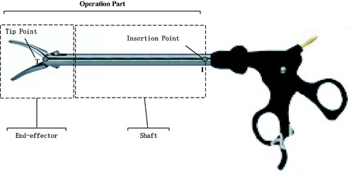
The operation part of conventional MIS instruments can be subdivided into end-effector and shaft portions (Figure 1), each having a corresponding key point, which needs to be pre-determined or estimated. The shaft portion has one important constraint point named “insertion point” (denoted as I in Figure 1), which is defined as the shaft axis and cavity wall intersection. The 2D/3D locations of insertion point can be pre-determined using the method described elsewhere [7,23]. Since the end-effector portion has a shape of pliers (Figure 1) with a tip moving during the surgical process, its tip point cannot be set at the tip true location and, instead, is assigned as a point between the shaft and pliers (denoted as T in Figure 1), whose 2D position or image position is to be estimated by the trained CNN of the proposed tracking-by-detection framework. We define the 2D tracking-by-detection problem as estimation of the parameters (˜n,˜T), and the 3D estimation problem as determination of the parameters (n,T), where n is direction of the line segment TI, ˜n is its image, and ˜T is the image of tip point T. For each new input video frame, we estimate the image direction ˜n via the newly proposed long-line segment extraction algorithm, and the imaged tip position ˜T via the well-trained CNN. Based on the 2D image parameters, the 3D ones (n,T) are derived.

Figure 1. The operation part of MIS instrument: end-effector with the tip point and shaft with the insertion point.

RANSAC-based line feature extraction for shaft detection

Due to self-evident availability of two long-line edges for the shaft portion of instrument in the image, the line feature is chosen to describe it. The general procedure of line detection [24] starts from detection of edge-points in the image with their further grouping into lines, which is mostly achieved within framework of the Hough transform approach by analysing the processed image and finding the lines, e.g. using the Probabilistic Hough Transform Hough-Lines-P software. Although the edge-point detection with processing of all pixels in the image is always heavy-computational and the voting process of Hough transform is time-consuming and unsuitable for the fast or real-time detection, the efficient detection of line features can be provided without processing each individual pixel of the image. In the proposed procedure, a line-detector is presented, which makes use of a spare sampling of the image data to find the candidate edge-points for lines, and then utilizes the RANSAC grouper to find line segments consistent with those edge-points. The RANSAC scheme finds an object pose from 3D-2D point correspondences: in order to fit lines passing through a set of edge-points, it randomly selects two edge-points, fits a line through them, and measures the number of inliers, i.e. edge-points that lie within a threshold distance to the line. The process is repeated for several samples, and the lines with the sufficient number of inliers are then chosen.

The proposed method of edge-point detection utilizes an efficient way of searching for edge-points in a rough grid of image pixels, which has widely spaced rows and columns (also named horizontal and vertical scanlines). Every two adjacent rows or columns are located 5 pixels apart from each other. Along each scanline, the Gaussian derivative is used to estimate each pixel gradient. If the gradient local maximum exceeds a certain preset threshold value (e.g. set as 0.12), the respective pixel is treated as the edge-point. The orientation of each edge-point is estimated by taking arctan (g_v/g_u), where g_v and g_u are two components of the gradient.

Each input video frame is split into a number of small image regions (40×40 pixels), wherein two edge-points with orientations within a preset angle (e.g. ) are chosen randomly for the RANSAC grouper analysis. The number of edge-points supporting each putative line is calculated, while the edge-points located at a close distance (0.1–0.3 pixels) to the line and having the inclination angle less than with the line are considered as the inliers of the line. After several short line segments are detected in each small region, they are subjected to the merging process, wherein two individual short line segments are merged together, if their orientations are compatible (within ) and their distance is less than 3 pixels. Finally, two long lines are constructed with the maximum merging number of short line segments. These two long lines correspond to the instrument shaft portion. The intersection point of these two long lines can be denoted in homogeneous coordinates via the estimated parameter ˜n.

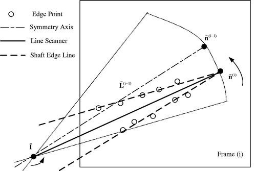
In case the above procedure has already been applied to the previous frame (i-1) and yielded the value ˜n^(i-1), the respective value ˜n⁽ⁱ⁾ of the next/current frame (i) can be derived in a more efficient way, as follows. An image line scanner is constructed to rotate around the image point of I. As shown in Figure 2, the scanning range is restricted to a sector area with the symmetry axis ˜L^(i-1), which satisfies the condition ˜L^(i-1)=˜I+s˜n(i-1), where ˜I is the image of I, and s is an arbitrary scale. The scanning angle can be chosen in the range between and , and the scanning step size is taken as . At every step, the number of line scanner inliers is calculated. Along all the scanning steps, there are two steps where the line scanner has the maximum number of inliers. At each of the two steps, the supporting edge points are used to start a RANSAC grouper, and a long image line is fitted. The two long image lines correspond to the shaft two edge lines, whose intersection point is the estimated ˜n⁽ⁱ⁾.

Figure 2. Line scanner application for detection of shaft edge lines and shaft image direction estimation.

End-effector detection based on CNN

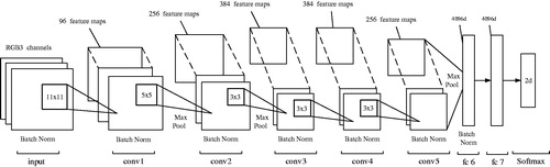
The structure of end-effector portion of surgical instrument is quite complex, so it is difficult to find an existing image feature (even local invariant features, e.g. HoG and SIFT) for proper description of the end-effector portion in video sequences. Deep networks, such as convolutional neural networks (CNNs), which can directly learn features from raw video data without resorting to manual tweaking, are widely used in the state-of-the-art applications involving such intricate tasks as object recognition, detection and segmentation and demonstrate the outstanding performance in representing visual data. Therefore, in this study, the end-effector detection was performed using the CNN (Figure 3), which is actually a modified AlexNet [25] consisting of 5 convolutional layers (denoted as conv1∼conv5) and 2 fully connected ones (denoted as fc6 and fc7). The batch normalization (denoted as Batch Norm) is added to all layers, except for fc7, to prevent the internal covariate shift. The layer conv1 has 96 feature maps, each of conv2 and conv5 layers have 256 feature maps, while each of conv3 and conv4 has 384 feature maps. The layer fc6 and fc7 are all 4096-dimentional. Three kinds of filters are used in the CNN with the size of 11×11, 5×5 and 3×3. All filters’ weights are updated through a training process. These trained weights of filters are actually the feature descriptions of the end-effector portion in some scale spaces. For offline training, 700 positive (end-effector) and 700 negative (background) samples were collected from video sequences. The sample size is 101×101. For the positive samples, the image centre of every sample is set at the imaged tip position ˜T. The network with batch size equal to 50 was trained for 20 epochs with learning rates of 10e-4 for the convolutional layers and of 10e-3 for the fully connected layers.

Figure 3. The CNN architecture for the end-effector detection consisting of 5 convolutional (conv1 ∼ 5) and 2 fully connected (fc6 ∼ 7) layers.

The searching path of end-effector detection is 1 D and is much simpler than the traditional 2D scanning strategy (left to right, top to bottom). For the current frame (i), the bounding box (˜p,s) slides along the symmetry axis ˜L⁽ⁱ⁾ obtained by shaft detection, from point ˜n⁽ⁱ⁾ to insertion point ˜I. The parameter ˜p is the centre of bounding box, which is on the line ˜L⁽ⁱ⁾. The parameter s is the scale factor of the bounding box. The image in the bounding box at every sliding step with scale s is resized to 101×101 and then used as an input for the trained CNN. The highest score of the CNN positive output corresponds to the bounding box (˜p⁽ⁱ⁾,s⁽ⁱ⁾), where ˜p⁽ⁱ⁾ is treated as the imaged tip position ˜T⁽ⁱ⁾ of the current frame (i).

Estimation of 3D parameters for the surgical instrument

Before the procedure of tracking-by-detection, the camera of endoscope should be calibrated using the Zhang method [26], so the internal matrix K of endoscope should be already derived. The camera model of endoscope is commonly reduced to the well-known pinhole model (1) where X is a 3D point in the world frame, ˜x is the corresponding image point on the image plane, d is the depth factor, [R|t] is the external matrix. Without loss of generality, we assume that the world frame coincides with the camera one, so Equation (1) takes the following form (2)

For the known image direction ˜n⁽ⁱ⁾, we can estimate the 3D parameter n⁽ⁱ⁾ as (3)

Then the relation L⁽ⁱ⁾=I+sn(i), where s is an arbitrary scale, will hold for the 3D symmetry axis L⁽ⁱ⁾. Since the 3D point T⁽ⁱ⁾ is located at the line L⁽ⁱ⁾, we can derive T⁽ⁱ⁾ as follows: (4)

Experimental results

To verify the proposed method feasibility, several test experiments similar to those in [17,27,28] were conducted on a controlled platform, where a printout of a surgical scene was taken as background, while the surgical instrument moved randomly in the view of endoscope. Under such conditions, the method was applied to track/detect the surgical instrument in 2D and 3D spaces. Furthermore, the results obtained were compared to those reported in a recent state-of-the-art study [7], and qualitative evaluation was also provided for in-vivo video sequences. The method was implemented via the Matlab R2014a and the above computation program was successfully realized using a PC with a 2.9 GHz dual-core CPU and Windows 7 system.

Ex-vivo test results

Using the above platform and experimental setup, the ex-vivo sequences were collected via an Olympus endoscope. Since the true instrument trajectories in 2D and 3D spaces cannot be acquired without the support of optical tracking system and robotic encoder, the Zhao method [7], which is accurate, robust, and readily realized in the real-time scale, was selected to track the 2D and 3D locations of instrument in our sequences, with the tracking results considered as the benchmark. The CNN training was made using a set of image samples randomly selected from some reference sequences, the number of samples (positive and negative) being 720. Prior to tracking procedure, a single video of the instrument motion was recorded, based on which the insertion point 2D and 3D coordinates could be estimated using the method described in detail elsewhere [8]. Since floating of the insertion point is inevitable in real surgeries, the floating error compensation is provided by the random noise application random noise to the insertion point estimated position during tracking.

The evolutions of 2D and 3D positions of the end-effector tip were measured during the tracking process. In Figure 4, the trajectories of 2D end-effector tip obtained by the proposed and reference ([7]) methods are plotted in the u-v-frame space. Figure 5(a–c) show the 3D trajectories of end-effector tip for these two methods in the camera frame. The errors of the proposed method to the reference one in the X-Y-Z coordinates are depicted in Figure 6 and listed in Table 1, while selected frames from the tracking procedure of the proposed method are shown in Figure 7.

Figure 4. The 2D trajectories of end-effector tip obtained by the proposed method (solid lines) and that in [7] (dash-dotted lines).

Figure 5. The end-effector tip 3D trajectories in X-Y-Z coordinates.

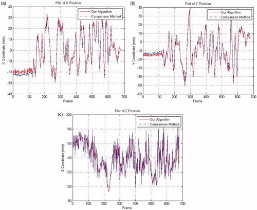
Figure 6. The end-effector tip 3D errors in the X-Y-Z coordinates.

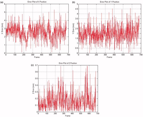
Figure 7. Selected frames of the instrument tracking and detection: the red circles are the tracked end-effector tip position, and the green dashed line is the shaft symmetry axis.

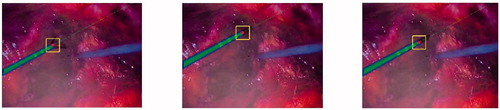
Table 1. The mean errors and standard deviations for 2D/3D numerical results obtained by the proposed method.

	3D errors (mm)			2D errors (pixel)
	X	Y	Z	u	v
Mean	2.5697	1.9701	0.3545	3.1417	2.7073
Std. Dev.	0.8172	0.8076	0.1984	3.7129	3.0085

In-vivo test results

To verify the qualitative results of the proposed method, some experiments were conducted based on several in-vivo sequences captured in some training operations of the medical school provided by the TIMC-IMAG laboratory. Based on these in-vivo video data, the proposed tracking algorithm and the comparison method [7] were also implemented via the Matlab R2014a using a PC with a 2.9 GHz dual-core CPU and Windows 7 system.

Since the analysed in-vivo data were not captured via the platform and experimental setup used for ex-vivo ones, the camera parameters of endoscope remained unknown and the 3D position of insertion point could not be estimated, thus making impossible the implementation of method [7]. A failure to obtain the 3D tracking data did not prevent the 2D tracking by the proposed method, which yielded some tracking frames of our algorithm (Figure 8). The 2D measurement errors between our algorithm and the comparison method [7] are listed in Table 2.

Figure 8. Example frames of in-vivo sequences with the end-effector positions shown by squares.

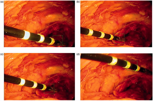
Table 2. The 2D mean errors and standard deviations of in-vivo test.

	2D errors (pixel)
	u	v
Mean	6.1695	5.2378
Std. Dev.	5.9261	5.4736

Discussion

The experiments with ex-vivo video sequences strongly suggest the state-of-the-art tracking performance and improved tracking accuracy of the proposed method, as compared to available ones. As is seen in Figure 4 and Table 1, the 2D discrepancies errors between the two methods are small: the mean errors are less than 4 pixels. The comparison of 3D trajectories in Figure 5 and Table 1 proves their close fit: the mean errors in X-Y-Z directions are less than 3 mm, while their standard deviations imply the proposed method’s strong robustness to noise interference. As shown in Figure 6, the maximal 3D error of the proposed method is about 5 mm, which is even less than the mean error in [9]. The collinear hypothesis used in the Equation (4)(4) accounts for the small errors in X-Y coordinates: insofar as the insertion point is included in the estimation of tracking position, the errors of Z coordinates are well-controlled (less than 1 mm).

Compared with those of ex-vivo test, the 2D measurement errors of in-vivo test are at least 2.5 pixels higher both in (u, v). Due to less strict requirements to illumination conditions in training operations, in contrast to the real ones, the in-vivo video sequences are little dimmer than the ex-vivo ones. When the respective 2D tracking by the proposed method was also applied to each frame with the CNN-based detection of instrument, the insufficient illumination of the image part (end-effector) accounted for drifted tracking results in some frames (see Figure 8(a,d)), which is the main reason why the in-vivo test has higher 2D measurement errors. Since the CNN training data did not include any samples from in-vivo video sequences, the trained CNN failed to identify the real instrument image in the bounding box of some frames, invoking drifted tracking results, which issue can be resolved by adding samples of in-vivo sequences into the training database.

Actually, the MIS instrument’s translation, rotation, and more generic warping are not fully considered during the tracking process of our algorithm. The spatial transformation of MIS instrument in tracking can lead to less accuracy of classification, so the 2D tracking errors of our algorithm in both ex-vivo and in-vivo tests are higher than 2.7 pixels, which might be improved by applying some regression CNN based on transformation invariant constraints.

Conclusion

In this study, novel method of surgical instrument tracking-by-detection is proposed, which considers the surgical instrument as two parts: end-effector and shaft, each being provided a different feature description, whereas the edge-points and line features are used for the shaft detection of shaft, and the trained CNN (deep learning) features are proposed to track and detect the end-effector. Due to a seamless combination of the above two feature description procedures, the resulting tracking method exhibits a better performance than the available ones. Further refinement of the proposed method will focus on dealing with the conditions of occlusion and multi-instruments, which is planned to be achieved by constructing a more efficient and robust line feature detector and a more flexible CNN structure.

Acknowledgements

The authors would like to thank TIMC-IMAG for supplying the ex-vivo and in-vivo laparoscope data.

Disclosure statement

No potential conflict of interest was reported by the authors.

Additional information

Funding

This work has been supported by the Specialized Research Fund for the Doctoral Program of Higher Education of China (No. 20130131120036), the Promotive Research Fund for Excellent Young and Middle-aged Scientists of Shandong Province (No. BS2013DX027), the National Natural Science Foundation of China (No. 81401543, 61673244), the French National Research Agency (ANR) through TecSan Program.

References

- Stoyanov D. Surgical vision. Ann Biomed Eng. 2012;40:332–345.
- Yang W, Hu C, Meng M, et al. A 6D magnetic localization algorithm for a rectangular magnet objective based on a particle swarm optimizer. IEEE Trans Magn. 2009;45:3092–3099.
- Joskowicz L, Milgrom C, Simkin A, et al. Fracas: a system for computer-aided image-guided long bone fracture surgery. Comput Aided Surg. 1998;3:271–288.
- Wei G, Arbter K, Hirzinger G. Automatic tracking of laparoscopic instruments by color coding. In: Joint Conference Computer Vision, Virtual Reality and Robotics in Medicine and Medical Robotics and Computer-Assisted Surgery. Heidelberg (BER): Springer; 1997. p. 357–366.
- Krupa A, Gangloff J, Doignon C, et al. Autonomous 3-d positioning of surgical instruments in robotized laparoscopic surgery using visual servoing. IEEE Trans Robot Automat. 2003;19:842–853.
- Bouarfa L, Akman O, Schneider A, et al. In-vivo real-time tracking of surgical instruments in endoscopic video. Minim Invasive Therapy. 2012;21:129–134.
- Zhao Z. Real-time 3D visual tracking of laparoscopic instruments for robotized endoscope holder. Bio-med Mater Eng. 2014;24:2665–2672.
- Wolf R, Duchateau J, Cinquin P, et al. 3D tracking of laparoscopic instruments using statistical and geometric modeling. In: 14th International Conference on Medical Image Computing and Computer-Assisted Intervention-MICCAI. Heidelberg (BER): Springer; 2011. p. 203–210.
- Agustinos A, Voros S. 2D/3D real-time tracking of surgical instruments based on endoscopic image processing. In: 2nd International Workshop on Computer Assisted and Robotic Endoscopy-CARE. Heidelberg (BER): Springer; 2015. p. 90–100.
- Dockter R, Sweet R, Kowalewski T. A fast, low-cost, computer vision approach for tracking surgical tool. In: 2014 IEEE/RSJ International Conference on Intelligent Robots and Systems-IROS. Chicago (IL); 2014. p. 1984–1989.
- Pezzementi Z, Voros S, Hager DG. Articulated object tracking by rendering consistent appearance parts. In: 2009 IEEE International Conference on Robotics and Automation-ICRA. Kobe; 2009. p. 3940–3947.
- Reiter A, Allen PK. An online learning approach to in-vivo tracking using synergistic features. In: 2010 IEEE/RSJ International Conference on Intelligent Robots and Systems-IROS. Taipei; 2010. p. 3441–3446.
- Li Y, Chen C, Huang X, et al. Instrument tracking via online learning in retinal microsurgery. In: 17th International Conference on Medical Image Computing and Computer-Assisted Intervention-MICCAI. Heidelberg (BER): Springer; 2014. p. 464–471.
- Reiter A, Allen PK, Zhao T. Feature classification for tracking articulated surgical tools. In: 15th International Conference on Medical Image Computing and Computer-Assisted Intervention-MICCAI. Heidelberg (BER): Springer; 2012. p. 592–600.
- Allan M, Thompson S, Clarkson MJ, et al. 2D-3D pose tracking of rigid instruments in minimally invasive surgery. In: 5th International Conference on Information Processing in Computer-Assisted Interventions-IPCAI. Heidelberg (BER): Springer; 2014. p. 1–10.
- Du X, Allan M, Dore A, et al. Combined 2D and 3D tracking of surgical instruments for minimally invasive and robotic-assisted surgery. Int J Cars. 2016;11:1–11.
- Wesierski D, Wojdyga G, Jezierska A. Instrument Tracking with Rigid Part Mixtures Model. In: 2nd International Workshop on Computer Assisted and Robotic Endoscopy-CARE. Heidelberg (BER): Springer; 2015. p. 22–34.
- Sznitman R, Richa R, Taylor RH, et al. Unified detection and tracking of instruments during retinal microsurgery. IEEE Trans Pattern Anal Mach Intell. 2013;35:1263–1272.
- Richa R, Balicki M, Sznitman R, et al. Vision-based proximity detection in retinal surgery. IEEE Trans Biomed Eng. 2012;59:2291–2301.
- Bourdev L, Malik J. Poselets: body part detectors trained using 3D human pose annotations. In: 2009 International Conference on Computer Vision-ICCV2009. Kyoto; 2009. p. 1365–1372.
- Fischler MA, Bolles RC. Random sample consensus: a paradigm for model fitting with applications to image analysis and automated cartography. Commun Acm. 1981;24:381–395.
- Fukushima K. Analysis of the process of visual pattern recognition by the neocognitron. Neural Netw. 1989;2:413–420.
- Doignon C, Nageotte F, de Mathelin M. The role of insertion points in the detection and positioning of instruments in laparoscopy for robotic tasks. In: 9th International Conference on Medical Image Computing and Computer-Assisted Intervention-MICCAI. Heidelberg (BER): Springer; 2006. p. 527–534.
- Clarke JC, Carlsson S, Zisserman A. Detecting and tracking linear features efficiently. In: 7th British Machine Vision Conference. Edinburgh; 1996. p. 415–424.
- Krizhevsky A, Sutskever I, Hinton GE. Imagenet classification with deep convolutional neural networks. Adv Neural Inf Process Syst. 2012;25:1097–1105.
- Zhang Z. A flexible new technique for camera calibration. IEEE Trans Pattern Anal Machine Intell. 2000;22:1330–1334.
- Wang W, Zhang P, Shi Y, et al. Design and compatibility evaluation of magnetic resonance imaging-guided needle insertion system. J Med Imaging Health Inform. 2015;5:1963–1967.
- Wang W, Shi Y, Goldenberg A, et al. Experimental analysis of robot-assisted needle insertion into porcine liver. BME. 2015;26:S375–S380.