A new hand-eye calibration approach for fracture reduction robot

Abstract

Objective: The hand-eye calibration is used to determine the transformation between the end-effector and the camera marker of the robot. But the robot movement in traditional method would be time-consuming, inaccurate and even unavailable in some conditions. The method presented in this article can complete the calibration without any movement and is more suitable in clinical applications. Methods: Instead of solving the classic non-linear equation AX = XB, we collected the points on X and Y axes of the tool coordinate system (TCS) with the visual probe and fitted them using the singular value decomposition algorithm (SVD). Then, the transformation was obtained with the data of the tool center point (TCP). A comparison test was conducted to verify the performance of the method. Results: The average translation error and orientation error of the new method are 0.12 ± 0.122 mm and 0.18 ± 0.112° respectively, while they are 0.357 ± 0.347 mm and 0.416 ± 0.234° correspondingly in the traditional method. Conclusions: The high accuracy of the method indicates that it is a good candidate for medical robots, which usually need to work in a sterile environment.

Keywords:

• Hand-Eye Calibration
• singular value decomposition
• fracture reduction robot

Introduction

There have been many developments in computer-assisted orthopedic surgery over the years. Presently, numerous robots are used for computer-aided navigation in orthopedic trauma surgeries. In robot-assisted fracture reduction, hand-eye calibration is a critical step that determines the spatial relation between the robot end-effector (hand) and the camera (eye) mounted onto the end-effector. The spatial relation is usually represented by a homogeneous matrix, which consists of a rotational component and a translational component; the robot analyses the matrix to know the exact position of end-effector in camera space.

In general, a homogenous transform equation of the form AX = XB can be established when the robot moves once [1]. In this equation, A is the transform matrix of the tool coordinate system (TCS) in the robot; B is the transform matrix of the camera, and X is the transform matrix that extends from the TCS of the robot to the camera. Tomasi et al. [2] reported that to establish the uniqueness of the solution, it is sufficient to prove that two calibration motions occur with non-parallel rotation axes. Numerous methods were proposed to solve this equation. Shiu et al. [1] solved the equation by decoupling the rotational part from the translational part (equation 1(1) , 2(2) ); the after-processed formulations were simple, fast but error-prone. Chen [3] solved the equation without decoupling the rotational and translational parts for the first time; the solution was based on the concept of screw motion. Daniilidis [4] introduced dual quaternions—an algebraic representation of the screw theory to describe motions. Using dual quaternions, Daniilidis was able to find a solution for the rotation and translation. Andreff et al. [5] formulated a self-calibration process by combining the structure-from-motion methods with the known robot motions. Using structure-from-motion methods, the camera poses were obtained solely from a camera-recorded image sequence. A calibration pattern was not needed to perform this technique, so it was suitable for clinical applications [6]. (1) (2)

In the above equations, R_A, R_B, R_X are the rotational terms of the homogeneous transformation matrix of A, B, and X; are the translational terms.

Both the movement of the robot and the camera can affect the calibration results of real applications. To obtain an accurate calibration result, the robot and camera often have to undergo a big movement; however, a big movement is not convenient in some situations. Moreover, the calibration process may be time-consuming. For the fracture reduction robot, the hand-eye calibration has to be performed every time before surgery in order to maintain sterile conditions. Furthermore, the robot cannot move to complete the intraoperative calibration, because the patient’s limb has been fixed on the platform.

In this study, we proposed a new approach for performing a rapid hand-eye calibration in robot-assisted fracture reduction. Using the singular value decomposition algorithm (SVD), we fitted the X and Y axes of the TCS directly with the points collected by the visual probe. Then, the transformation was obtained easily with the data of the tool center point (TCP). In this way, the whole calibration process was performed only in the camera space without moving the robot. Thus, the calibration time was significantly reduced with this new approach. Compared with the traditional method, our novel method showed good accuracy and efficiency. In clinical applications, our method would be the most preferable choice.

This paper is organized as follows: In Section II, we present the mathematical algorithm of the traditional method and our line fitting method. In Section III, we describe the experiments carried out using the two different methods. Then, we also present the results of these experiments. In Section IV, we provide an analysis of the experimental results. In Section V, we present a conclusion of our work.

Materials and methods

System overview

Figure 1 illustrates the system used for performing lone bone fracture reduction surgery. The critical components are the operation bed, fracture reduction robot (6 degrees of freedom (DOF) parallel robot), and the optical tracking system (Hybrid Polaris Spectra, Northern Digital Inc, Canada) [7–9]. The hand-eye calibration was performed before the operation, and it was used to determine the spatial relationship between the TCS of the reduction robot and the marker coordinate system (MCS) on the platform. Figure 2 illustrates these two coordinate systems, namely, TCS and MCS. To complete the fracture reduction operation, a parallel robot analyzes this spatial relationship under the guidance of the optical tracking system.

Figure 1. The reduction robot system.

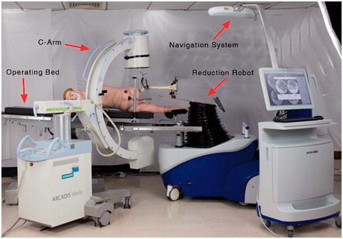
Figure 2. The coordinate systems of the reduction robot.

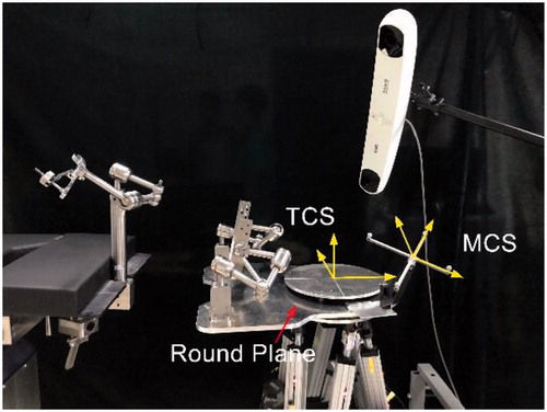
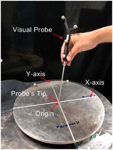
During the calibration phase, the TCS of the reduction robot was set elaborately on a round plane; the X and Y axes of TCS were grooved on the round plane, so they were easily detected by the tip of the visual probe. Figure 3 illustrates the details of the round plane.

Figure 3. The details of the round plane.

AX = XB method

The eq. (1)(1) can be written as follows: (3)

Let n_B be the eigenvector of R_B, which is associated with the unit eigenvalue. Then, multiply eq. (1)(1) with n_B: (4)

According to eq. (4)(4) , R_Xn_B is the eigenvector of R_A, which is associated with the unity unit eigenvalue (n_A). (5)

Now, the homogenous transform equation AX = XB is equivalent to eq. (2)(2) and eq. (5)(5) .

Equation (2)(2) and eq. (5)(5) represent one motion of the hand-eye device. Two such motions are necessary to obtain the rotational and translational parts. In the general case of n motions, the solution of such 2n equations would minimize two positive error functions. (6) (7)

The problem of simultaneously estimating the rotational and translational parts can be described in terms of the following minimized problem: (8)

Several special minimization methods have been designed specifically to deal with this case. Among them, the Levenberg-Marquardt method and the trust-region method are good candidates.

Using unit quaternions, the minimum error function is expressed in the following form of quaternions: (9)

Where (10)

There are two techniques for solving the non-linear minimization problem of eq. (9)(9) . In the first technique, eq. (9)(9) is considered as a classical non-linear least squares minimization problem; and it is solved using standard non-linear optimization techniques, such as Newton’s method and Newton-like methods. In this article, the results were calculated using the Levenberg-Marquardt non-linear minimization algorithm [10]. The second technique is to try to simplify the expression of the error function for minimization. Using the properties of quaternions, we can simplify the error function.

SVD method

The X and Y axes of TCS were engraved in the end-effector of fracture reduction robot, so it was easily detected by the visual probe. Thus, we determined the spatial relationship of TCS and the visual marker without moving the robot. The calibration had high efficiency and accuracy. We collected the points on the X and Y axes and fitted them with 3 D lines, which are known as 3 D Orthogonal Distance Regression (ODR) line [11–13]. Then, we used the SVD algorithm to calculate the rotational term. The translational term was obtained directly from the origin of TCS in the camera space. The following process was used to calculate the translational term:

The visual probe was used to collect the raw 3 D points of axis:  1 vectors).

The average of each axis is given by the following expression: (11)

Each point subtracts the p_ave and we get These vectors compose the matrix M: (12)

Then we used the SVD algorithm as follows: (13)

The direction of the fitting line is as follows: (14) where v₁ is the first column vector of the orthogonal matrix V.

The direction vectors l_x,l_y of X and Y axes were obtained using the collected points of the X and Y axes, respectively. Because the system was orthogonal, we could obtain the direction vector l_Z of Z axis using eq. (15)(15) : (15)

The translational term of TCS to MCS can be obtained as follows: (16)

The final transformation matrix is given by the following expression: (17)

Experiments and results

Experiments based on AX = XB method

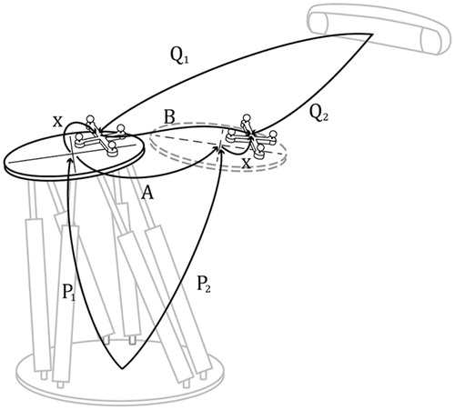
In this method, the robot moved step by step by following the given transformation matrix sequences (A₁,A₂,⋯A_n). After each movement of the robot, the tracking system captured the marker’s transformation matrices (P₀,P₁,⋯P_n) in the camera space (see Figure 4). Please note that the robot’s transformation matrices should match the marker’s transformations. The marker frame transformation B_i was formulated in eq. (18)(18) . For the accuracy of the results, the robot moved 10 steps totally. The whole process took about six minutes. (Note: The fracture reduction robot is a six DOF parallel robot whose repeated positioning accuracy is less than 0.05 mm. Moreover, its positioning accuracy is much higher than the camera accuracy; therefore, we ignored the influence of robot’s error.) (18)

Figure 4. Hand-eye calibration via traditional method.

Experiments based on the SVD method

We captured the transformations of the probe in the camera space (T_probe^camera ) using the optical tracking system. Figures 5(a) and 5(b) show that the probe slide followed the groove of X and Y axes on the plane. As shown in Figure 5(c), the probe’s tip was then placed on the origin of TCS (the intersection of the two grooves on the round plate) to collect the original position data. This process is necessary because the data is used to determine the translational term of the transformation. During the data collection process, we could adjust the posture of the probe as long as the probe’s tip was in contact with the bottom of the groove. We calculated the position of probe’s tip in camera space using the following expression: (19)

Figure 5. Collecting the points positions of the axis and origin.

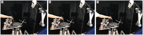
Here P_tip^probe is the position of the tip in the probe coordinate system, and it is a constant for a specific probe.

The probe’s tip in marker space is calculated using the following equation: (20)

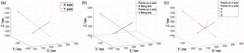
All the data was collected in one minute. Figure 6(a) shows the scattered points collected in MCS, and Figure 6(b) shows the fitting line obtained using SVD algorithm. Figure 6(c) shows TCS in MCS.

Figure 6. (a) The scattered points collected in MCS. (b) The fitting line of points obtained using SVD. (c) TCS in MCS.

Results

Because the real transform is unknown, we could not directly calculate the errors between the real hand-eye transform and the computed one. Therefore, the following method was used to rate the quality of the resulting transformation: when the robot moved one step, we got an estimate of the marker movements ε′ from the computed value of hand-eye transformation X. This estimated movement ε′ was compared with the original marker movement ε obtained using the optical tracking system [6].

We decomposed the marker movements into the euler angle and translation. The error distribution of the two different methods used to analyze 20 motions is shown in Table 1 and Figure 7. The average translation error and orientation error of the new method are 0.12 ± 0.122 mm and 0.18 ± 0.112° respectively, while they are 0.357 ± 0.347 mm and 0.416 ± 0.234° correspondingly in the traditional method. The results indicate that SVD algorithm is more accurate and stable than the traditional method.

Figure 7. The error distribution analysis in translation and rotation.

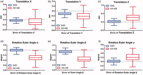
Table 1. The standard deviation of eular and translation.

	Method	α/°	β/°	γ/°	tX/mm	tY/mm	tZ/mm
Mean	AX = XB	−0.3026	−0.1866	0.2157	−0.0745	−0.2190	0.2715
	SVD	−0.091	−0.0885	0.1376	−0.0285	−0.1130	0.0289
Standard deviation	AX = XB	0.1263	0.0679	0.1846	0.1691	0.1686	0.2524
	SVD	0.0539	0.0673	0.0719	0.0519	0.0630	0.0905

Discussion

To determine the spatial relationship between the robot end-effector and the camera, the conventional approach is to use a homogeneous transformation equation AX = XB; The equation is solved to obtain the rotational and translational terms either individually or simultaneously [1,14]. Moreover, some extension studies based on AX = XB are also in progress, such as transforming the equation to AX = YB [15]. These techniques are applicable in most situations; however, the calibration process can become cumbersome in clinical applications, because it has to be done before each operation so as to comply with the sterile requirement. Moreover, the traditional method cannot be used in the intraoperative calibration, because the patient’s limb is fixed on the fracture reduction robot.

The SVD algorithm is an important matrix factorization in linear algebra. It is generally used for matrix diagonalization in matrix analysis. It is primarily used in signal processing applications, statistics, and other fields [16–18]. Because our fracture reduction robot has a special design, its TCS can be reached easily using the visual probe and the optical tracking system, which then directly calculate the hand-eye transformation matrix. Thus, we eliminated the errors associated with robot’s motions and equation solving methods. The experimental results indicate that our new method is more accurate and efficient than the conventional method that involves solving of the AX = XB equation.

The drawback of this method is that it can only be used on a particular type of robots; the TCS of these robots was marked on the end-effector, so they could be touched easily by the probe. This requirement could not be met easily in a normal serial robot, because the gripper is usually mounted onto the end-effector.

Conclusion

We proposed a new method for performing the hand-eye calibration of fracture reduction robot. With this method, we could obtain the hand-eye transformation matrix without solving the non-linear equation AX = XB. After fitting the axis of TCS using SVD algorithm, we calculated the transformation matrix directly in this method. The whole process was conducted in the camera space without moving the robot. Therefore, this calibration method is very reliable and time-saving. The experimental results of this method were compared with those of the traditional techniques. The results clearly indicated that the new method is more accurate than traditional one. All these characters are critical in clinical applications, because the hand-eye transformation matrix has to be calibrated every time before conducting the surgery in order to meet the sterile requirement. We can do this calibration now, because the TCS of this medical robot can be reached easily; however, it may be difficult in other serial robots. In the latter situations, it is better to solve the equation AX = XB.

Disclosure statement

No potential conflict of interest was reported by the authors.

Additional information

Funding

This work was supported by National Hi-Tech Research and Development Program of China (“863” Project) (Grant Nos. 2015AA043204), National Natural Science Foundation of China (No. 61333019), and National Science and Technology Major Project of the Ministry of Science and Technology of China (2014ZX04013011).

References

- Shiu YC, Ahmad S. Calibration of wrist-mounted robotic sensors by solving homogeneous transform equations of the form AX = XB. IEEE Trans Robot Automat. 1989;5:16–29.
- Tsai RY, Lenz RK. A new technique for fully autonomous and efficient 3D robotics hand/eye calibration. IEEE Trans Robot Automat. 1989;5:345–358.
- Chen HH. A screw motion approach to uniqueness analysis of head-eye geometry. Proceedings CVPR’91, IEEE Computer Society Conference on Computer Vision and Pattern Recognition; 1991, Jun 3; p. 145–151.
- Palaniappan K, Fraser J. Multiresolution tiling for interactive viewing of large datasets. In: 17th Int. Conf. on Interactive Information and Processing Systems (IIPS) for Meteorology, Oceanography and Hydrology; 2001. p. 338–342.
- Andreff N, Horaud R, Espiau B. Robot hand-eye calibration using structure-from-motion. Int J Robot Res. 2001;20:228–248.
- Schmidt J, Vogt F, Niemann H. Calibration–free hand–eye calibration: a structure–from–motion approach. Paper presented at Joint Pattern Recognition Symposium; 2005 Aug 31. p. 67–74.
- Du H, Hu L, Li C, et al. Advancing computer-assisted orthopaedic surgery using a hexapod device for closed diaphyseal fracture reduction. Int J Med Robotics Comput Assist Surg. 2015;11:348–359.
- Wang T, Li C, Hu L, et al. A removable hybrid robot system for long bone fracture reduction. Biomed Mater Eng. 2014;24:501–509.
- Du H, Hu L, Li C, et al. Preoperative trajectory planning for closed reduction of long-bone diaphyseal fracture using a computer-assisted reduction system. Int J Med Robotics Comput Assist Surg. 2015;11:58–66.
- Press WH, Teukolsky SA, Vetterling WT, etet al. Numerical recipes in C. Cambridge: Cambridge University Press; 1996.
- Mandel J. Use of the singular value decomposition in regression analysis. Am Statist. 1982;36:15–24.
- Golub GH, Reinsch C. Singular value decomposition and least squares solutions. Numer Math. 1970;14:403–420.
- Boggs PT, Rogers JE. Orthogonal distance regression. Contemp Math. 1990;112:183–194.
- Ma Q, Li H, Chirikjian GS. New probabilistic approaches to the AX = XB hand-eye calibration without correspondence. IEEE International Conference on Robotics and Automation (ICRA), 2016 May 16. p. 4365–4371.
- Li H, Ma Q, Wang T, et al. Simultaneous hand-eye and robot-world calibration by solving the $AX = YB $Problem without correspondence. IEEE Robot Autom Lett. 2016;1:145–152.
- Rufai AM, Anbarjafari G, Demirel H. Lossy image compression using singular value decomposition and wavelet difference reduction. Digital Signal Process. 2014;24:117–123.
- Nilashi M, bin Ibrahim O, Ithnin N. Multi-criteria collaborative filtering with high accuracy using higher order singular value decomposition and Neuro-Fuzzy system. Knowledge-Based Syst. 2014;60:82–101.
- Makbol NM, Khoo BE, Rassem TH. Block-based discrete wavelet transform-singular value decomposition image watermarking scheme using human visual system characteristics. IET Image Process. 2016;10:34–52.