A segmentation of brain MRI images utilizing intensity and contextual information by Markov random field

Abstract

Background and objective: Image segmentation is a preliminary and fundamental step in computer aided magnetic resonance imaging (MRI) images analysis. But the performance of most current image segmentation methods is easily depreciated by noise in MRI images. A precise and anti-noise segmentation of MRI images is desired in modern medical image diagnosis.

Methods: This paper presents a segmentation of MRI images which combines fuzzy clustering and Markov random field (MRF). In order to utilize gray level information sufficiently and alleviate noise disturbance, fuzzy clustering is carried out on the original image and the coarse scale image of multi-scale decomposition. The spatial constraints between neighboring pixels are modeled by a defined potential function in the MRF to reduce the effect of noise and increase the integrity of segmented regions. Spatial constraints and the gray level information refined by Fuzzy C-Means (FCM) algorithm are integrated by maximum a posteriori Markov random field (MAP-MRF). In the proposed method, the fuzzy clustering membership obtained from the original image and the coarse scale image is integrated into the single-site clique potential functions by MAP-MRF. The defined potential functions and the distance weight are introduced to model the neighborhood constraint with MRF.

Results: The experiments are carried out on noised synthetic images, simulated brain MR images and real MR images. The experimental results show that the proposed method has strong robustness and satisfying performance. Meanwhile the method is compared with FCM, FGFCM and FLICM algorithms visually and statistically in the experiments. In the comparison, the proposed method has achieved the best results. In the statistical comparison, the proposed method has an average similarity index of 36.8%, 33.7%, 2.75% increase against FCM, FGFCM and FLICM.

Conclusions: This paper proposes a MRI segmentation method combining fuzzy clustering and Markov random field. The method is tested in the noised image databases and comparison experiments, which shows that it is a precise and robust MRI segmentation method.

Keywords:

• Brain MRI
• image segmentation
• maximum a posteriori Markov random field

1. Introduction

In recent years, medical images acquisition methods have developed rapidly, including methods such as magnetic resonance imaging (MRI), X-ray computer tomography (CT), ultra-sound (US), positron emission tomography (PET) and single photon emission tomography (SPET). As an increasing number of medical images are produced, automatic image processing and analysis techniques have become essential [1–3]. MRI is one of the most commonly utilized medical imaging techniques. It provides good contrast for dissimilar tissues and offers predominance over CT and other diagnostic imaging techniques for brain tissue studies, making it an attractive method for most image segmentation researchers.

The purpose of image segmentation is to partition an image into mutually exclusive regions, each of which has homogeneous properties that are significantly different from those of the neighboring regions. In the field of medical images, development of brain image segmentation is an important research area [4]. Cerebrospinal fluid (CSF), gray matter (GM) and white matter (WM) are the principal components of the brain and they are the main targets for image segmentation in brain MR images. In clinical applications, accurate segmentation of brain tissues can facilitate searching and analysis of position, type and extent of physiological changes in the brain. Accurate tissue segmentation can be used to obtain quantitative results of physiological change, which can be used for data mining based on quantitative analysis [5–8]. In brain tumor imaging, brain tumor segmentation can be used to identify the size and location of the tumor. The tumor state and progress of tumor growth can also be obtained by quantitative analysis and comparison.

Many MRI image segmentation methods have been developed in recent years, including statistical models [9], active control models [10], atlas-based methods [11] and clustering methods. Fuzzy clustering-based image segmentation is one of the most efficient and widespread methods for MRI image segmentation. The Fuzzy C-Means (FCM) algorithm is the most popular among fuzzy clustering methods, and is a clustering algorithm introduced by James [12]. It is based on minimizing an object function by iteratively updating the membership function and cluster centers. FCM has been proven to work well on most noise-free medical images, but it is very sensitive to noise within the medical image. This is due to the fact that the FCM algorithm only utilizes the gray level information of each pixel and ignores spatial contextual information. Many improved algorithms based on FCM have been developed, which are directed at using image spatial context information sufficiently, to address the defects in the standard FCM algorithm.

A fuzzy rule-based scheme called the ruled-based neighborhood enhancement system was developed in [13], which imposed spatial constraints on the image during post-processing of the FCM clustering results. Ahmed et al. [14] modified the objective function of the standard FCM algorithm to allow the labels in the immediate neighborhood of a pixel to influence its labeling and the algorithm was named FCM_S. However, incorporation of neighborhood information was limited to single-feature inputs. Cai et al. [15] proposed the fast generalized FCM algorithm (FGFCM) which incorporates local spatial and gray information together. It can alleviate the flaws of FCM_S while simultaneously enhancing the clustering performance. [16] presented a variation of the standard FCM method, which incorporated the local spatial information and gray level information by using a fuzzy local (both spatial and gray level) similarity measure to guarantee noise insensitivity and image detail retention. In [17], an adaptive spatial information-theoretic fuzzy clustering algorithm was presented to improve the robustness of the standard FCM method.

The modified FCM methods described above have improved the performance for noisy images by utilizing spatial information. Since noise is independent of location, spatial constraints can reduce noise disturbance. However, the smoothing effect of the spatial information can lose details in the original image when it suppresses noise. Therefore, rational and proper utilization of spatial information for image segmentation is critical.

Markov random field (MRF) theory has been widely used in image segmentation and analysis [18]. It can facilitate modeling of spatial or contextual dependencies in images. Ashraf et al. [19] presented a methodological framework for multi-channel MRFs. Under this framework, the kinetic feature maps derived from breast dynamic contrast-enhanced MRIs were incorporated as observation channels in the MRF for tumor segmentation. A notable improvement was shown compared with the standard FCM and enhanced FCM methods. [20] proposed a method based on MRF and a hybrid of social algorithms, including an ant colony optimization and a Gossiping algorithm, which can be used for segmenting MRIs in real time environments. In [21], based on an assumption that modeling the image content locally rather than globally could provide a more accurate classification result, a framework was introduced for tissue classification in brain MRI based on local, MRF-based image models.

As described in the aforementioned literature, FCM is a good tool to analyze and utilize luminance information from images and MRF can facilitate modeling of the spatial or contextual dependencies in the images. Therefore it may be a feasible idea to combine FCM and MRF to carry out medical image segmentation. This combination has been implemented recently in some applications. [22] proposed a fuzzy treatment of hidden MRF model-based image segmentation. In [23], they applied FCM with the MRF for change detection in synthetic aperture radar (SAR) images. They classified changed and unchanged regions using FCM with a defined Markov random field energy function. An improved method for color texture image segmentation based on fuzzy c-means clustering and region-level MRF model was proposed in [24]. [25] proposed a multispectral and panchromatic images fusion approach exploiting local spatial information by using FCM clustering algorithm based on the MRF. For medical image segmentation, we propose a MRI segmentation method combining fuzzy clustering and Markov random field. It is different from [23] that modified the fuzzy clustering membership of each pixel by MRF energy function, we preserve the standard form of FCM and integrate it into MAP-MRF framework as the gray level information extraction and analysis component in our algorithm.

The rest of this paper is organized as follows. Section 2 describes the preliminary theory in relation to FCM and MRF, and details of the proposed algorithm. Experimental and comparison results are presented in Section 3 and we conclude this paper in Section 4.

2. Methods

2.1. Fuzzy C-means clustering

The fuzzy c-means algorithm [12] is based on minimizing the objective function which is the weighted sum of squared error of the clusters: (1) (2) where X={x₁,x₂,…,x_N} is the data set and x_i⊆ℝ^K in the K-dimensional vector space, N is the number of data items, c is the number of clusters with 2≤c≤N, u_ij is the degree of membership of x_i belong to the j^th cluster, m is the weighting exponent on each fuzzy membership, v_j is the prototype of the center of cluster j and d²(x_i,v_j) is the distance between data x_i and cluster center v_j.

Using the Lagrange Multiplier and constrain in Equation (2)(2) , the derivatives of u_ij and v_j in J(U,V) can be found: (3) (4)

The minimization of objective function J_m can be obtained by iteratively updating the membership function and cluster center.

2.2. The MAP-MRF framework

Markov random field theory provides a convenient and consistent way of modelling context-dependent entities such as image pixels and correlated features [26]. The maximum a posteriori Markov random field (MAP-MRF) framework is advocated by Geman for statistical image analysis problems [27]. For segmentation, it can be considered to be a labeling problem and the segmented result can be retrieved by seeking the maximum a posteriori estimation of the labeling problem.

Let the rectangular lattice for a 2 D image of size M×N be defined as follows: (5)

For a lattice S, the set of neighbors of element i is defined as the set of sites within a radius of from i (6)

Clique c in S defined as a subset of sites in S. Single-site clique c={i}, pair-site clique c={i,i^′}, triple-site clique c={i,i^′,i^″}, (i,i^′,i^″∈S and neighbor each other), and so on. The collections of all single-site cliques, pair-site cliques, and triple-site cliques can be denoted as C₁,C₂ and C₃. The collection of all cliques C=C₁∪C₃∪C₃…

In MAP-MRF framework, the MRI segmentation can be converted to a labeling problem which gives different labels to pixels e.g. WM, GM, CSF etc. The joint probability of each pixel’s label in the MR image is modeled by the MRF, denoted by (7) where, N and M are the height and the width of the MR image in pixels. S={(m,n)|1≤m≤M,1≤n≤N},f_i∈S∈{1,…,L_K}, where i is a pixel in S, and L_K,k∈1,…,K, corresponding to labels of the different tissues in the brain. According to markovianity, for each i∈S, P(f_i|f_S-{i}) equals to P(f_i|f_Ni), where N_i denotes the neighborhood system of i. By the Hammersley-Clifford theorem, (8) where, d=d₁,…,d_M*N is the observation, Z and T are constants. The energy function (9) is the sum of clique potentials V_c(f|d) over all possible cliques in C. Then, the solution of the original segmentation or labelling problem can be denoted as: (10)

The computation would take a long time if calculated over all cliques. In practice, execution of the computation over single site cliques and pair site cliques is widely adopted. In other words, the second-order neighborhood system is adopted, where the label of i is only decided by the elements in N_i={i^′∈S|[dist(pixel_i^′,pixel_i)]²≤2,i^′≠i} and i itself. In this situation, the model is also called an auto-model [28].

2.3. Segmentation based on fuzzy clustering and MRF

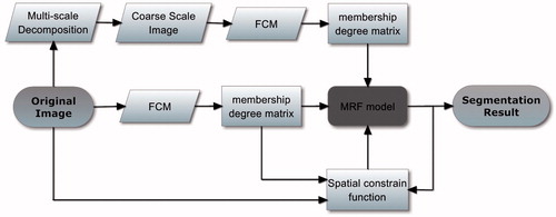
FCM has been proven to be an efficient method in medical image segmentation. Improvement of FCM is focused on that introduces pixels spatial constraint information by modifying the membership or objective function [13–17]. MRF is a formal and powerful tool for modeling mutual influences among image neighboring pixels and has undergone extensive theoretical development [18–21,23,26]. In this paper, a MRI segmentation method which combines fuzzy clustering and a Markov random field is proposed. Under MAP-MRF framework with a defined spatial constraint potential function, the fuzzy clustering membership degree information is introduced to improve segmentation performance. Additionally, the fuzzy clustering membership is also retrieved from coarse scale image of multi-scale decomposition of the original image to alleviate noise disturbance and enhance robustness. The block diagram of the proposed algorithm is shown in Figure 1.

Figure 1. Block diagram of proposed algorithm.

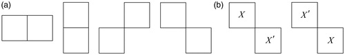
The cliques C utilized in this paper include single-site clique C₁ (i itself) and pair-site clique C₂ [Figure 2(a)], C=C₁∪C₂. The MRF is assumed to be isotropic and homogeneous, where V_c(f_i|d_i^′) is unrelated with the position of i in S and U(f|d) is unrelated with the clique direction, as shown in Figure 2(b). In other words, the potential function V_c(f) should have the same value at (X_,X^′) and (X_′,X). The neighborhood system N_i, has eight immediate spatial neighboring pixels. In this paper, the potential function is defined as (11)

Figure 2. Neighborhood system's pair-site clique: (a) Pair-site clique. (b) Isotropy.

where, potential function V_C1(f_i,d_i) is on a single-site clique and V_C2(f_i,f_i^′) is on a pair-site clique, and we calculate all spatial neighboring blocks on a pair-site clique.

2.3.1. Single-site clique potential function V_C1(f_i,d_i)

The single-site clique potential function provides the supporting information for the final segmentation decision from the location i itself. In this paper, the supporting information from location i is retrieved mainly from FCM membership. (12) where λ₁ and λ₂ are the coefficients.

A) Single-site clique potential function on the original image

We define the potential function on single-site clique as below (13) where u_i,j is the fuzzy clustering membership degree of i belong to the class j. L_k is the class label, k={1,2,3,4} and L={BG,GM,WM,CSF}.

B) Single-site clique potential function on coarse scale image

The coarse scale image is obtained using wavelet transform on the original image. Applying the FCM method on the coarse scale image produces another fuzzy partition matrix U_coarse. (14) μ_coarse is the element in the fuzzy partition matrix U_coarse.

2.3.2. Pair-site clique potential function V_C2(f_i,f_i^′)

The pair-site clique potential function provides the supporting information for the final segmentation decision from the spatial neighbors of location i. (15) where λ₃ and λ₄ are the coefficients.

A) Potential function on degree of membership of spatial neighbors

Based on the assumption of spatial consistency, the value of each pixel should be closed to the value of neighboring pixels, i.e., the membership degree of the current pixel to a certain class would be closed to its neighbors’. We define the potential function on the membership degree of spatial neighbors as shown below: (16) where N_i is the spatial neighbors of i. abs(⋅) is the absolute value function. d_i,i^′ is the distance between pixel i and its neighbor i^′ and d_i,i^′ is the weight that reflects the extent of influence from neighbors.

B) Potential function on classes of spatial neighbors

Each current pixel i most likely to be segmented to the same class as most of its neighbors, or each pixel i is most likely in the same region as its neighbors. We then define the potential function on classes of spatial neighbors as shown below: (17) where I_i is the gray level of pixel i and L_i is the label (class) of pixel i.

2.4. Coefficients fixing

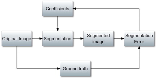
The coefficients λ₁, λ₂, λ₃ and λ₄ are intrinsically represents the contribution of each partial information of the original image to final segmentation result. These coefficients are needed to be defined for different type images(e.g. synthetic images or MRIs). In this paper, these coefficients are learned ahead using prepared images to enhance the segmentation performance. The learning process is needed only once to calibrate the coefficients for the same type images. The coefficients fixing process shows in Figure 3. In the process, the coefficients are fixed just at the least segmentation error.

Figure 3. Coefficients fixing process flow scheme.

2.5. MRF model solution

There are several algorithms that can be used to solve the MRF model. ICM is used in this study. The ICM method firstly assigns original labels, and enumerates a label set 1,…,L_K to calculate U(f_i) exhaustively, replacing f_i^k with f_i^k+1 such that U(f_i) is minimized iteratively until f_i^k+1=f_i^k,i∈S.

Original labels setting is an important step in ICM. A popular choice is maximum-like estimation: In this paper, the segmented result of FCM can be initialized using the original labels to reduce the number of iterations.

3. Experimental results and analysis

Experiments are carried out on three image databases: synthetic images, simulated MRI images and real MRI images. There are four MRI image segmentation algorithms used and compared in experiments, which are FCM [12], FGFCM [15], FLICM [16] and the proposed method. All executed algorithms are programmed in Matlab (version 2006), with the exception of the main procedure of FLICM algorithm, which is programmed using programming language C which provides a dynamic link library. The proposed method is appraised by quantitative indexes and visual comparison.

To quantitatively evaluate the performance of segmentation, there are three indexes (similarity index ρ, false positive ratio r_fp and false negative ratio r_fn) [29] employed in the experiment. For segmentation of a given image, let A_i and B_i represent the sets of pixels belonging to class i in the “ground truth” and the segmentation result respectively. |A_i| denotes the number of pixels in the set A_i. The similarity index is a legible index to calculate matched pixels between A_i and B_i, which is defined as (18)

The false positive ratio r_fp represents errors due to misclassifications of class i and the false negative ratio r_fn represents errors due to the loss of desired pixels of class i; These are defined as follows: (19) (20)

In these experiments, we set the neighborhood size N=3×3 for all algorithms except the standard FCM.

3.1. Synthetic images

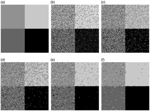
A synthetic square image (256×256) is generated in this section, which consists of four squares. The intensity values of the four squares are 0, 100, 145, and 199, respectively [see Figure 4(a)]. Noise obeys a Rician distribution in MRI images. However, if only the signal to noise ratio isn’t low, a quasi-Gaussian distribution can be used to approximate the noise [30]. The noisy images segmented in this experiment are obtained by adding 5% Gaussian white noise [see Figure 4(b)] and 10% Gaussian white noise [see Figure 5(b)].

Figure 4. Experiment on synthetic image: (a) Original Image. (b) Original Image with Gaussian noise (5%). (c) FCM result. (d) FGFCM result. (e) FLICM result. (f) Proposed method result.

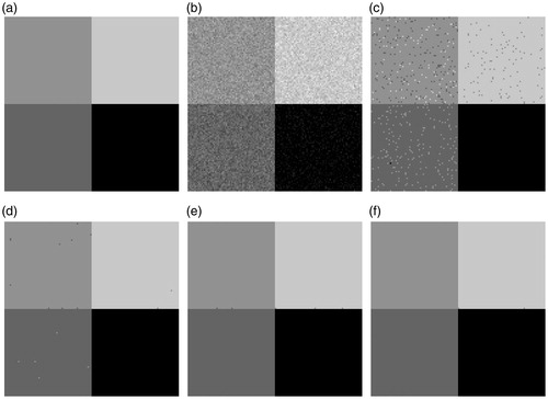
Figure 5. Experiment on synthetic image: (a) Original Image. (b) Original Image with Gaussian noise (10%). (c) FCM result. (d) FGFCM result. (e) FLICM result. (f) Proposed method result.

3.1.1. Visual comparison

Figure 4 shows the original image [Figure 4(a)], a noisy image (original image with 5% Gaussian white noise) [Figure 4(b)] and the segmentation results on the noisy image [Figure 4(c-d)]. With 5% added noise [Figure 4(b)], each algorithm achieves a satisfactory result, with the exception of FCM [see Figure 4(c)]. There are still a few misclassified pixels are shown in the segmented result using the FGFCM algorithm [Figure 4(d)]. The FLICM method segmented result in [Figure 4(e)] shows that very few visually misclassified pixel blocks exist. Figure 4(f) shows the segmented result using the method that is proposed in this paper. Visually, there is no obvious segmentation errors in the segmented result.

Figure 5 shows the experiment on the original image with 10% Gaussian white noise. In this experiment, the noise disturbance can't be considered to be negligible for each algorithm. Visually, the proposed method has the least noise interference.

3.1.2. Statistical comparison

Using the definitions for the similarity index ρ, false positive ratio r_fp and false negative ratio r_fn as given in Equations (18)(18) , Equation (19)(19) and Equation (20)(20) , we compare the four algorithms quantitatively. For index ρ is always less than one and a larger value corresponds with a better algorithm. For indexes r_fp and r_fn, a smaller value corresponds with a better algorithm. Table 1 shows the indexes for each segmentation result of the original image with 5% Gaussian white noise, corresponding to the visual results in Figure 4. The right-most column of the table shows the average value of indexes. The Table 1 shows that the proposed algorithm has relatively better performance. The average of ρ achieves the highest value, while r_fp and r_fn maintain the lowest level. Additionally, this table shows the similarity index ρ of the proposed method is above 99.9% for the four squares. It can be seen that the proposed method is robust and provides with better performance in the synthetic image than other methods

Table 1. Indexes of different methods in synthetic (5%) images.

Methods	Index	0	100	145	199	Average
FCM	ρ	0.9999	0.9539	0.9307	0.9764	0.9652
	rfp	0.0002	0.0442	0.0723	0.2246	0.0348
	rfn	0	0.0479	0.0667	0.0246	0.0348
FGFCM	ρ	1	0.9982	0.9979	0.9998	0.999
	rfp	0	0.0024	0.0017	0	0.001
	rfn	0	0.0012	0.0024	0.0005	0.001
FLICM	ρ	1	0.9998	0.9994	0.9996	0.9997
	rfp	0	0.0005	0.0007	0	0.0003
	rfn	0	0	0.0005	0.0007	0.0003
Proposed method	ρ	1	1	0.9998	0.9998	0.9999
	rfp	0	0	0.0005	0	0.0001
	rfn	0	0	0	0.0005	0.0001

Table 2 shows the indexes for each algorithms segmentation results of the original image with 10% Gaussian white noise, corresponding to the visual result in Figure 5. The table shows that all four algorithms achieve relatively lower performance than themselves in previous experiment, and disparities between indexes for each algorithms larger. This demonstrates that each segmentation algorithm is affected by the increased noise but that the proposed algorithm showed relatively less decrease in performance.

Table 2. Indexes for different methods in synthetic (10%) images.

Methods	Index	0	100	145	199	Average
FCM	ρ	0.8773	0.5781	0.509	0.6754	0.66
	rfp	0.1335	0.4399	0.6477	0.1558	0.3442
	rfn	0.1143	0.4146	0.4375	0.4106	0.3442
FGFCM	ρ	0.9503	0.6868	0.5886	0.743	0.7422
	rfp	0.082	0.3052	0.552	0.1008	0.26
	rfn	0.0205	0.3174	0.3528	0.3494	0.26
FLICM	ρ	0.9838	0.8648	0.8179	0.9297	0.899

3.2. Simulated images

Brainweb [31] is a simulated brain MRI database that includes a set of realistic MRI data volumes produced by an MRI simulator. In the database, we retrieved the “ground truth” of each tissue in the MRI volumes and simulated volumes under different types of conditions, such as noise level, slice thickness and so on. We were then able to utilize this data to estimate the performance of diverse image segmentation methods compared to the known “ground truth”. In this experiment, we execute four algorithms on a simulated data volume with T1-weighted sequence from Brainweb, slice thickness of 1 mm, volume size of 217×181×181. All algorithms partition the image into four classes: background, CSF, GM and WM. In the statistical result, background is ignored.

3.2.1. Visual comparison

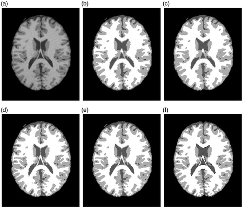
The brain image shown in Figure 6(a) is a slice (90th slice) of the simulated three dimensional volume with 3% noise of Rician. The experimental results of segmented by FCM, FGFCM, FLICM and proposed method can be seen in Figure 6(b-e), respectively. Figure 6(f) is the “ground truth” of Figure 6(a). The differences between the segmented results of each algorithm are not visually obvious. For some details, e.g., the center of the brain image should approximate this as a white color triangle. However, in Figure 6(b-c) the triangle lacks integrity, whereas in Figure 6(d-e) the triangle is visually obvious and closes to the ground truth.

Figure 6. Experiment on simulated image: (a) Original Image (simulated with 3% noise). (b) FCM result. (c) FGFCM result. (d) FLICM result. (e) Proposed method result. (f) Ground truth.

3.2.2. Statistical comparison

Table 3 shows the statistical results of the experiment shown in Figure 6. The table shows that the proposed method achieves a relatively better result across the averaged of the three defined indexes. Although the segmented image is corrupted by 3% noise, our result provides similarity indexes ρ of all three tissues that are larger than 93%. So our segmentation result has much more overlap with the “ground truth” than other methods.

Table 3. Indexes for different methods in simulated (3%) images.

Methods	Index	CSF	GM	WM	Average
FCM	ρ	0.8758	0.8691	0.929	0.8913
	rfp	0.1509	0.1543	0.0516	0.1189
	rfn	0.1034	0.113	0.0878	0.1014
FGFCM	ρ	0.8561	0.8898	0.9519	0.8993
	rfp	0.1645	0.1164	0.0409	0.1073
	rfn	0.1285	0.1053	0.0546	0.0961
FLICM	ρ	0.8822	0.9069	0.956	0.915
	rfp	0.095	0.1241	0.0335	0.0842
	rfn	0.1359	0.0674	0.0535	0.0856
Proposed method	ρ	0.9168	0.9344	0.9705	0.9406
	rfp	0.0782	0.088	0.0228	0.063
	rfn	0.0873	0.0459	0.0358	0.0564

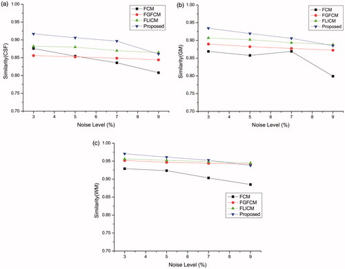
In order to further estimate our algorithm's performance on diverse noise levels, we repeat the experiment shown in Figure 6 on simulated MRI images with noise levels 5%, 7% and 9% respectively. The statistical results of the similarity index ρ show in Figure 7. Figure 7(a-c) show the segmentation of CSF, GM and WM in the experiments respectively. In each graph, the vertical axis represents the similarity index ρ and the horizontal axis represents the noise level. From the graphs, we can see that our method is almost the best at each noise level. Since the other three methods contain noise restrain processing with the exception of the standard FCM method, performance of the other three methods decreases more slowly as noise level increases.

Figure 7. Experiment on simulated image with different noise level: (a) CSF. (b) GM. (c) WM.

3.3. Real images

The proposed algorithm is also evaluated on a real MRI image. A normal T1-weighted real MRI brain volume (IBSR_01, size of 256×256×128) is downloaded from IBSR [32] by the Center for Morphometric Analysis at Massachusetts General Hospital. To facilitate the development and evaluation of the segmentation algorithm, the manually guided expert segmentation results are acquirable along with brain MRI image. We also tested algorithms on our own produced MRI images (512×512×432). In this study, all four algorithms partition real MR Images into four classes: background, CSF, GM and WM.

3.3.1. Visual comparison

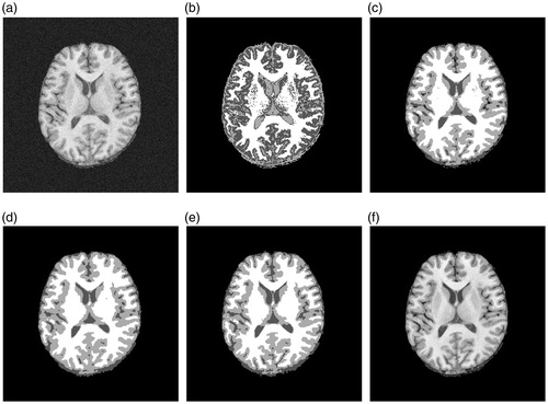
Figure 8(a) shows a normal T1-weighted real MRI image with noise (174th slice of the volume). The segmentation experiment results of FCM, FGFCM, FLICM and proposed method are shown in Figure 8(b-e) respectively. Figure 8(f) is the “ground truth” of Figure 8(a). There is a high volume of noise in Figure 8(b) using the standard FCM method. In Figure 8(c), compared with Figure 8(b), the noise has been restrained but it is still not satisfactory. Figure 8(d,e) show the segmentation results of the FLICM method and the proposed method. Since it is difficult to perform a visual evaluation, we can compare the results statistically.

Figure 8. Experiment on real MRI image: (a) MRI image with noise. (b) FCM result. (c) FGFCM result. (d) FLICM result. (e) Proposed method result. (f) Ground truth.

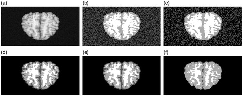
Figure 9 shows experimental results on own produced MRI images. Figure 9(a) shows the image with noise. The segmentation results on Figure 9(a) by FCM, FGFCM, FLICM and proposed method are shown in Figure 9(b-e) respectively. Figure 9(f) is the original image of Figure 9(a) without noise. In the results, a better segmentation are obtained in Figure 9(e), which is interfered least by noise compared to the other results.

Figure 9. Experiment on own real MRI image: (a) MRI image with noise. (b) FCM result. (c) FGFCM result. (d) FLICM result. (e) Proposed method result. (f) Original MRI image without noise.

3.3.2. Statistical comparison

Table 4 shows the statistical results of the four algorithms shown in Figure 8(a). In Table 4, the statistical result of the background is ignored. The right-most column of Table 4 provides the average index value, which shows that the proposed algorithm exhibits a slight advantage to FLICM method and achieves the best performance of all four algorithms. For the three individual segmented tissues (CSF, GM and WM), the proposed method also shows the best performance of all four algorithms, as shown in the corresponding columns in the table.

Table 4. Indexes for different methods in real MRI images.

Methods	Index	CSF	GM	WM	Average
FCM	ρ	0	0.7018	0.6824	0.4614
	rfp	20.5714	0.0965	0.9307	7.1995
	rfn	1	0.4072	0	0.4691
FGFCM	ρ	0.0095	0.6786	0.6677	0.4519
	rfp	13.3168	0.1003	0.9954	4.8042
	rfn	0.9317	0.435	0	0.4555
FLICM	ρ	0.4883	0.8095	0.892	0.7299
	rfp	2.014	0.0134	0.2105	0.746
	rfn	0.0264	0.3109	0.0254	0.1209
Proposed method	ρ	0.4911	0.8212	0.8933	0.7352
	rfp	1.8913	0.0132	0.2032	0.7026
	rfn	0.059	0.2942	0.0289	0.1274

Table 5 shows the experimental results of the four algorithms executed on the 18 subjects in the IBSR database. In this table the proposed method still achieves best performance and slightly better than FLICM method. The experiment results also declare that the performance and robustness of the proposed method are validated.

Table 5. Indexes for different methods in IBSR database.

Methods	FCM			FGFCM			FLICM			Proposed method
Index	ρ	rfp	rfn	ρ	rfp	rfn	ρ	rfp	rfn	ρ	rfp	rfn
Average value	0.42	7.67	0.51	0.44	5.52	0.48	0.7	0.79	0.2	0.72	0.74	0.19

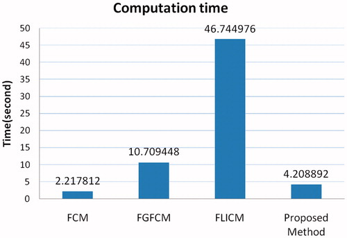
Figure 10 shows the computation time of the four algorithms on the own real MRI images. The proposed method consumes less time than FGFCM and FLICM method, and just falls behind the native FCM method.

Figure 10. Computation time of the four segmentation methods.

4. Discussion and conclusion

Robust and accurate Brain MRI segmentation is a key requirement in clinical practice and often also in medical research. FCM is a classical method applied in medical image segmentation and it has disadvantage of sensitive to noise within the medical image. To address the defects in the standard FCM algorithm, improved FCM methods have been developed, which are directed at using image spatial context information sufficiently, but rational and proper utilization of spatial information for image segmentation is critical. Meanwhile MRF is a perfect tool that can accurately model spatial or contextual dependencies in images. Hence executing the image segmentation through synthesizing the intensity information retrieved by the FCM and the contextual information extracted by the MRF will produces desirable results.

In this paper, we propose a MRI segmentation approach combining fuzzy clustering and Markov random field. The gray level information and the spatial information in the segmented image are retrieved and processed by FCM and MRF model respectively. The evaluation experiments in this paper show that the proposed method based on FCM and MRF is a feasible and effective approach to construct a robust and precise segmentation algorithm. The proposed approach integrates the fuzzy clustering membership of original image into MRF potential function as segmentation supporting information. It generates a fuzzy clustering membership from coarse scale image of multi-scale decomposition, which is integrated into the MRF potential function to alleviate noise disturbance. The defined potential functions and the distance weight are then introduced to reduce noise effect and support precise segmentation when modeling neighborhood constraints with MRF. In our experiments, we test the proposed approach on synthetic images, simulated MRI images and a real MRI image database. The experimental results show that the proposed approach improves the segmentation performance, as well as robustness against noise. And the proposed method achieves higher efficiency in the participant algorithms except the native FCM. Contextual Information is utilized by MRF in the proposed method, but only the single site and pair site clique are considered in the method. A larger range of spatial information and contextual information can be extracted from the MRI images to retrieve better segmentation result in the future improved algorithm.

Disclosure statement

No potential conflict of interest was reported by the author(s).

Funding

This work was supported by the Foundation of the Third Military Medical University [grant No. 2014XZH03], Chongqing Postdoctoral Science Foundation [grant No. Xm2015061], Youth Development Programs in Military Medical Technology [grant No. 15QNP060] and the National Natural Science Foundation of China [grant No. 61372065]. The funders had no role in the study design, data collection and analysis, decision to publish, or manuscript preparation.

References

- Bauer S, Wiest R, Nolte L, et al. A survey of MRI-based medical image analysis for brain tumor studies. Phys Med Biol. 2013;58:R97–R129.
- Zhuang X. Challenges and methodologies of fully automatic whole heart segmentation: a review. J Healthc Eng. 2013;4:371–407.
- Gordillo N, Montseny E, Sobrevilla P. State of the art survey on MRI brain tumor segmentation. J Magn Reson Imaging. 2013;31:1426–1438.
- Balafar MA, Ramli AR, Saripan MI, et al. Review of brain MRI image segmentation methods. Artif Intell Rev. 2010;33:261–274.
- West J, Blystad I, Engstrom M, et al. Application of quantitative MRI for brain tissue segmentation at 1.5 T and 3.0 T field strengths. PloS One. 2013;8:e74795.
- West J, Warntjes JBM, Lundberg P. Novel whole brain segmentation and volume estimation using quantitative MRI. Eur Radiol. 2012;22:998–1007.
- Flórez N, Bouzerar R, Moratal D, et al. Quantitative analysis of cerebrospinal fluid flow in complex regions by using phase contrast magnetic resonance imaging. Int J Imaging Syst Technol. 2011;21:290–297.
- Sled J, Nossin-Manor R. Quantitative MRI for studying neonatal brain development. Neuroradiology. 2013;55:97–104.
- Balafar MA. Gaussian mixture model based segmentation methods for brain MRI images. Artif Intell Rev. 2014;41:429–439.
- Wang L, Shi F, Li G, et al. Segmentation of neonatal brain MR images using patch-driven level sets. Neuroimage. 2014;84:141–158.
- Cabezas M, Oliver A, Lladó X, et al. A review of atlas-based segmentation for magnetic resonance brain images. Comput Methods Programs Biomed. 2011;104:e158–e177.
- JC. Bezdek Pattern recognition with fuzzy objective function algorithms. New York (NY): Springer US, 1981.
- Tolias YA, Panas SM. Image segmentation by a fuzzy clustering algorithm using adaptive spatially constrained membership functions. IEEE Trans Syst, Man, Cybern A. 1998;28:359–369.
- Ahmed MN, Yamany SM, Mohamed N, et al. A modified fuzzy c-means algorithm for bias field estimation and segmentation of MRI data. IEEE Trans Med Imaging. 2002;21:193–199.
- Cai W, Chen S, Zhang D. Fast and robust fuzzy c-means clustering algorithms incorporating local information for image segmentation. Pattern Recogn. 2007;40:825–838.
- Krinidis S, Chatzis V. A Robust Fuzzy Local Information C-Means Clustering Algorithm. IEEE Trans Image Process. 2010;19:1328–1337.
- Wang Z, Song Q, Soh YC, et al. An adaptive spatial information-theoretic fuzzy clustering algorithm for image segmentation. Comput Vis Image Underst. 2013;117:1412–1420.
- Scherrer B, Forbes F, Garbay C, et al. Distributed local MRF models for tissue and structure brain segmentation. IEEE Trans Med Imaging. 2009;28:1278–1295.
- Ashraf AB, Gavenonis SC. A multichannel markov random field framework for tumor segmentation with an application to classification of gene expression-based breast cancer recurrence risk,”. IEEE Trans Med Imaging. 2013;32:637–648.
- Yousefi S, Azmi R, Zahedi M. Brain tissue segmentation in MR images based on a hybrid of MRF and social algorithms. Medical Image Analysis. 2012;16:840–848.
- Tohka J, Dinov ID, Shattuck DW, et al. Brain MRI tissue classification based on local Markov random fields. J Magn Reson Imaging. 2010;28:557–573.
- Chatzis SP, Varvarigou TA. A fuzzy clustering approach toward Hidden Markov random field models for enhanced spatially constrained image segmentation. IEEE Trans Fuzzy Syst. 2008;16:1351.
- Gong M, Su L, Jia M, et al. Fuzzy Clustering With a Modified MRF Energy Function for Change Detection in Synthetic Aperture Radar Images. IEEE Trans Fuzzy Syst. 2014;22:98–109.
- Liu G, Li P, Zhang Y. A color texture image segmentation method based on fuzzy c-means clustering and region-level markov random field model. Math Probl Eng. 2015;2015:1.
- Liu J, Lei Y, Xing Y, et al. Multispectral and panchromatic images fusion using the Markov-random-field-based FCM. Remote Sens Lett. 2015;6:992–1001.
- Li SZ. Markov random field modeling in image analysis. New York: Springer-Verlag, 2009.
- Geman S, Geman D. Stochastic relaxation, Gibbs distributions, and the bayesian restoration of images. IEEE Trans Pattern Anal Mach Intell. 1984;6:721–741.
- Besag J. Spatial interaction and the statistical analysis of lattice systems. J R Stat Soc Series B. 1974;36:192–236.
- Zijdenbos AP, Dawant BM. Brain segmentation and white matter lesion detection in MRI images. Crit Rev Biomed Eng. 1994;22:401–465.
- Sijbers J, den Dekker AJ, Scheunders P, et al. Maximum-likelihood estimation of Rician distribution parameters. IEEE Trans Med Imaging. 1998;17:357–361.
- Kwan RKS, Evans A, Pike GB. MRI simulation-based evaluation of image-processing and classification methods. IEEE Trans Med Imaging. 1999;18:1085–1097.
- Rohlfing T. Image Similarity and Tissue Overlaps as Surrogates for Image Registration Accuracy: Widely Used but Unreliable. IEEE Trans Med Imaging. 2012;31:153–163.