Design and application of tumor prediction model based on statistical method^*

Abstract

Two prediction models for tumor prediction based on logistic regression and BP neural network were proposed in this paper; a sensitivity analysis of risk factors was also conducted. The two protocols will be implemented in the R language and demonstrated with relevant lung cancer data. Additionally, the two models are compared, verifying their accuracy and feasibility. Finally, a function is combined with R language, which can quickly achieve the above two programs. It is set up to obtain the tumor prediction model and the risk factors on the degree of correlation of the size of the disease. This method is convenient and practical and we hope it can be applied in the early discovery of cancer during future medicine.

Keywords:

• Tumor prediction model
• logistic regression neural network
• R language

1. Introduction

In our country, malignant tumor is a well-known cancer, such as lung and breast cancer, and has a high morbidity and mortality rate. It is a great threat to human life. An important research topic in modern medicine includes how to overcome the malignant tumor.

Although there are many cancer prevention and treatment methods, the input level of primary and secondary prevention of the tumor is still not enough. There is the lack of measures of feasible community prevention interventions. Additionally, the current technology for discovering primary cancer is still very scarce. Many cancer patients are diagnosed at the advanced stage, which is the primary reason leading to the high incidence and mortality rates of cancer. Therefore, early detection, early diagnosis, and early treatment are still the primary measures for enhancing the survival rate and reducing the mortality rate of cancer patients.

Thus, the establishment the tumor prediction model is very important. Currently, the establishment of the tumor prediction model has reached some achievements around the world. Among the tumor prediction model, the gray GM (1,1) model, the Cox proportional hazards regression model, the logistic regression model, the artificial neural network model, and their combined application are widely used.

The gray GM (1,1) model was used widely early on and is a system of uncertainty with the implementation of the forecast method. The Gray GM (1,1) model is simple, has no exact conditions for the probability distribution of sample contents, and was used to establish tumor prediction model. The predictive effect is good and the adaptability is strong. It can provide reference for the development of tumor prevention and treatment [1]. Like some prognostic models, the disadvantage is that Gray GM (1,1) cannot individually assess a single patient, and can only stratify risk for specific populations.

The cox proportional hazards regression model is widely used in cancer and other chronic disease prognosis analyses, and the cohort study explored the factors of the disease. The cox proportional hazards regression models have also been used to predict the risk of lung cancer [2]. It is a multivariate analysis method, has a more flexible application, and it cannot consider the survival time distribution. Objects of the observation of the study queue can be sooner or later, but the length of time can be inconsistent and has the ability to use censored data. It is excellent for both group and individual predictive models.

Currently, the logistic regression model is widely used to explore the risk components [3] or predictive morbidity of disease. The model commonly uses the function _, probability p = L(w′x + b), among them, w and b are parameters to be determined and x is the risk factor in the related dependent variable. However, because of the varying data, the dependent variable or risk factors may vary. Therefore, the logistic regression models have different predictive models for different malignancies. For example, there are predictive models of lung cancer risk based on gender and smoking history [4], as well as predictive models of cervical cancer death. Additionally, the logistic regression model also has many options for the same type of malignant tumor.

Nowadays, artificial neural networks have also been applied to the prediction of malignant tumors [5]; they have developed some very good results with the continuous development of science and technology. The BP neural network is a multilayer feedforward network in the artificial neural network trained by error back propagation algorithm, and it is currently one of the most widely used neural network models. In some lung cancer risk prediction, BP neural network showed a higher accuracy compared to logistic regression [6]. However, because the neural network cannot explain the variables, it is best to combine them with each other during practical application [7].

Although many mathematical prediction models for malignant tumors have been proposed, which model is best suited for a variety tumor types is still questionable [8]. The accuracy of the existing models for the different tumor predictions are different; each prediction model has advantages and disadvantages, making it unrealistic to establish a secure model to adapt to each tumor prediction. Therefore, lung cancer will be used as an example with the main use of logistic regression analysis of relevant data. This process will include the use of the R language to read and analyze the data on lung cancer statistics, as well as build the logistic regression model for the exploration of the risk factor and prediction of sick probability. As the program can be achieved by the R language design algorithm, it was found that the rapid establishment program of the prediction model of combination of a R language and logistic regression method. Moreover, the logistic regression has a wide range of applicability, so the model can be extended, rapidly analyzed, and can predict other models of tumors. In addition, the risk components obtained by the logistic regression method will be put into the BP neural network; this will be to analyze the sensitivity and find more accurate components of the risk factors and their correlation to the pathogenesis of the tumor. The accuracy of the above models are then verified, that way we have the design of the prediction model of the tumor based on the logistic regression model, as well as the sensitivity analysis of the tumor risk factors based on the neural network model. In the end, the above two schemes were packaged in R language and a function was set up to complete the process. The risk factors, prediction models, and predicted individual morbidity will be obtained as long as the sample data and the data to be predicted are inputted. This method is convenient and practical and we hope it can be applied in the early discovery of cancer for future medicine.

2. Logistics regression model

2.1 Introduction to logistic regression model

Logistic regression is a multivariate analysis of the relationship between independent and dependent variables when it is exploring the dependent variable as a binary or multivariate class. It belongs to the non-linear regression of probability, and is now being adopted as the most common model. It can be used to predict which factors are the risk factors leading to malignancy in tumor prediction. If a model has been established, it is possible to predict the different conditions of the independent variable and the probability of the disease according to the model. It has a good predictive correctness and practicability in solving the situation where the dependent variable is a directional variable.

2.2 Binary logistic regression model

The dependent variable in the model can be classified as binary or multiple. Whether or not people fall ill is the dependent variable in this paper, and if not it is a dichotomous variable.

The dependent variable is binary with values Y = 1 or Y = 0. The m independent variables that affect the value of y are respectively . Under the influence of the related factors, the probability of Y = 1 is Then the logistic regression model can be written as: (1)

Among them β₀ is the constant term, and is the partial regression coefficient.

Letting , then the logistic curves of Z and P are as follows (see figure 1):

It can be shown that the value of P tends to 1 when Z tends to +∞, and the value of P tends to 0 when Z tends to −∞. The P value changes between (0,1), and as the Z value changes, the symmetry S shape changes around the point (0,0.5).

Logit transformation:

is logit transformation of P. Through the logit transformation, the information of 0 ≤ P ≤ 1 can be transformed into information of −∞ < log it(P) < + ∞.

The logistic regression model can be converted to the following linear form by logit transformation: (2)

2.3 Logistic variable screening

Stepwise regression

In the real world, we usually want to choose a few influential factors, such as the independent variables from the relevant components which have effect on the dependent variable. The multiple regression analysis method is used to build the optimal equation to predict and monitor the dependent variable. The optimal equation is constructed in order to cover all of the relevant components that significantly influence the dependent variable in the regression equation, and to eliminate the relevant components which do not have a significant influence on the dependent variable. Stepwise regression is a regression analysis program that was constructed based on this idea. In all of the relevant components that are in accordance with size of its influence and significant level from high to low are inputted, one by one, into the regression equation. However, components that have an insignificant influence may not be incorporated into the regression equation from beginning to end. Moreover, the components that have been incorporated into the regression equation may also show obvious levels of decline when new components are incorporated, and will then be removed from the regression equation. The components that are incorporated or removed are a step of the gradual regression. Additionally, each step needs to be tested to ensure that there are no insignificant components, but only significant components, in the regression equation before new components are incorporated into the equation.

3. Introduction to BP neural network

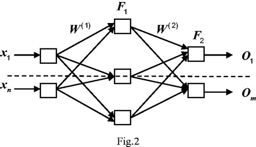
Actually, the BP algorithm can be described with the BP network with only one hidden layer. As shown in Figure 2, the structural model of the two stage BP neural network, input vector , ideal output vector , actual output vector , is connection weight of hidden layer, w⁽²⁾ is connection weight of output layer, F₁,F₂ are the hidden layer and the output layer activation function, F₁ uses a nonlinear Sigmoid function, F₂ uses a linear Purelin function, BP network learning is a mentor learning. The sample set is composed of vector pairs (x,y), that is input vector x, ideal output vector y, for a neuron, input: , the output of the neuron is: (3)

Figure 1. The logistic curves of Z and P.

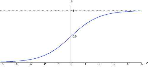
Figure 2. Model of two-layer BP network.

The learning process of BP network is divided into two stages:

3.1 Forward propagation stage

Take a sample () from the sample set, Enter x_p into the network;

Calculate the actual output o_p: hidden layer , output layer (4)

3.2 Backward propagation stage

1. Calculate the difference between the actual output and the desired output: (5)

2. Adjust the weight matrix by minimizing the error:

① Adjust connection weight of output layer :

② Adjust connection weight of hidden layer w⁽¹⁾: (6) where a is the learning rate, say the jth neural network input of output layer, say the kth actual output, say the h layer connection weights of the ith neurons to the jth neurons, h can be 1 or 2.

4. Numerical experiments

4.1 Specimen collection and data preprocessing

The data of this paper is obtained from the Heilongjiang Provincial Tumor Hospital. The data total consists of 400 cases. Among them are 250 patients with data and 150 patients without. By the selection, the relevant factors were identified as gender, age, smoking history, and history of respiratory diseases, such as chronic bronchitis. These factors are used in the following studies.

4.1.1 Setting of analysis of factors

Gender: male = 1, female = 2

Age: n

Smoking: do not smoke = 0, mild smoking = 1, severe smoking = 2

History of respiratory diseases: do not fall ill = 0, fall ill = 1.

4.1.2 Data preprocessing

① Read of data

Three data sets are set up in the paper, namely the training data set, test data set, and data set to be tested. The 400 data was randomly assigned to the training data set and the test data set, in which the training data set contains 300 cases of data, and the test data set contains 100 cases of data.

Training data set: building the model.

Test the data set: assisting model building, verifying models, and assessing model accuracy.

The data set to be tested: testing the correct functioning of the model.

The three data is stored in the same excel file among the different forms. You can directly use the form in the excel file with the help of the R language. This method is convenient and fast. The proposed algorithm does not limit the number of relevant factors at the end of the paper, only in the last column to store the dependent variable, that is, the disease or not. The algorithm analyzes the relationship of related factors between the last column and all of the preceding columns.

② Normalized data processing

Data normalization is the mapping of raw data to intervals or smaller intervals.

The role of normalization:

Due to the different physical parameters of each factor, and the large numerical differences, it is usually necessary to normalize all of the initial data in order to prevent large value messages from dropping small value information.

Not only can normalization improve the accuracy, but it can also ensure that speed of the convergence increases when the program is running.

B) Normalization algorithm:

The normalization algorithm chosen in this paper is a linear transformation algorithm. It is characterized by a simple and quick operation. (7)

In the above formula, X is the vector of input and Y is the vector of output. Min (X) and max (X) are the minimum and maximum values of X. The above equation maps the data into the [0,1] interval.

4.2 Model design based on logistic regression

4.2.1 Preliminary logistic regression analysis

The initial logistic regression analysis was performed by using the normalized training data set. The following is the relevant data analysis results that are obtained by the R language code.

However, the results of preliminary logistic regression analysis are not reliable. There may be multiple collinearities, and not all factors can pass the significance test. Therefore, further stepwise regression is required.

4.2.2 Logistic stepwise regression variable screening

Stepwise regression is performed by using the step function. The effects of multicollinearity can be eliminated, and uncorrelated factors are eliminated. The results are as follows.

4.2.3 Discussion on logistic regression results

The above results show that through gradual regression, age, smoking, and history of respiratory disease each passed the test. Simultaneously, we can obtain the logistic regression model of “disease-sex + age + smoking + history of respiratory disease”: , Linear form:

4.3 Sensitivity analysis of risk factors based on BP neural network

4.3.1 Setting and training of BP neural network

In this paper, the BP neural network model with the back propagation learning algorithm is adopted, and the training data set is normalized and trained. The model is constructed by the newff function in the R language. The network structure includes the input, hidden, and output layers. The parameters are set as follows.

The activation function of the hidden layer is Sigmoid (S-shaped curve): .

The activation function of the output layer is the linear function Purelin:

Error calculation: least mean square of adaptive gradient method

Learning rate: 1e-2

Number of hidden layer units: In this paper we construct the models of units with 1, 2, 3, (1,1), (1,2) and (2,1) in the hidden layer and test them on the test data set. The results show that (1,1) with two hidden layers has the highest accuracy in the measurement of correctness. Therefore, the final network structure is set to (3,1,1,1) and used for the following sensitivity analysis. We obtain the BP neural network prediction model as a result. Although there is no exact mathematical equation, it remains a good model for predicting the probability of having disease.

4.3.2 Sensitivity analysis of risk factors

The sensitivity analysis can determine which factors have a large impact on the system or model. The method is used to change the value of each variable in the sample. The system will record the maximum and minimum output and calculate the difference between the maximum and minimum values of the maximum output ratio. Finally, the sensitivity of the variable is all recorded the average of the ratios [9].

The results can be seen, risk factors: age, smoking, respiratory disease history, and the corresponding sensitivity: 0.17,0.48,0.69. Therefore, the above three risk factors can conclude that the impact of the size of the disease or not from small to large arrangement for the age, smoking, respiratory disease history.

4.4 Comparison and verification

4.4.1 Comparison and verification of prediction model accuracy

The accuracy of the logistic regression model was tested by validating the data set. The basic idea is that each of the individual data can be predicted for a total of n validation data, and the probability of disease is the ith is .

Among them are the m predicted values that are equal to the actual value of 0 or 1, then the accuracy rate is the proportion of the total m/n.

The final result is that 0.88 is the prediction accuracy rate of the logistic regression model, and 0.92 is the prediction accuracy rate of the BP neural network model. The BP neural network model has higher accuracy when compared with the logistic regression model.

4.4.2 ROC analysis

The receiver operating characteristic curve (ROC curve) is also known as the susceptibility curve. The ROC curve is plotted on a horizontal axis with the true positive rate (sensitivity) as the vertical axis and the false positive rate (1-specificity) as a series of different binary methods (cutoff or decision threshold). The original inspection and evaluation methods have the same characteristics, such as the experimental results will be reduced to two and then the statistical analysis is implemented. The ROC curve is evaluated in a manner that is different from the previous assessment without the above conditions. According to the realistic situation, the results of the ROC curve can be divided into several orderly categories, such as health, general health, undetermined, general abnormal, and abnormal five grades, and then then statistical analysis is implemented. Therefore, the evaluation method has a more general application.

The calculation of ROC curve evaluation [10]. The area under the ROC curve is between 1.0 and 0.5. If AUC > 0.5, then AUC is the closest to 1, showing a more accurate identification of results. If the AUC ∈(0.5,0.7), it means that the discrimination accuracy is low. If AUC ∈(0.7,0.9), it means that there is a specific accuracy. If AUC > 0.9, it means that the discriminant accuracy is higher. If AUC = 0.5, it means that the discriminant method has no effect, and there is no discriminant value. If AUC < 0.5, it means that it does not match the facts, and it generally does not occur. In theory, some scholars prove that AUC in the performance of the two-dimensional description of the component is more superior than the correct rate for the area under the ROC curve [11]. ROC curves of the two prediction models are shown in Figure 3.

Figure 3. ROC curves of two prediction models.

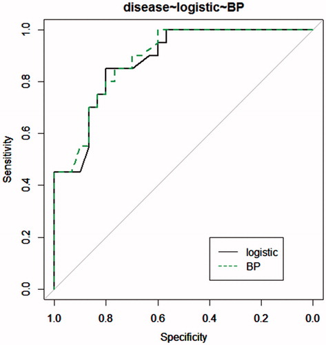
Figure 3 shows that the BP neural network model is more accurate than the logistic regression model.

The ROC analysis curves of each factor were drawn by using the R language in Figure 4.

Figure 4. ROC curve analysis.

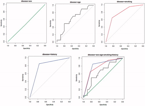
The results of the ROC curve in Figure 4 show that the relevant gender factors are independent variables, and the age, smoking, and respiratory disease history correlation is small to large, which is consistent with the sensitivity analysis.

Compared with the logistic regression model, the BP neural network model has higher accuracy, sensitivity analysis, and can better describe the effects of various factors on the prevalence. However, the model is unable to explain their arguments because there is not a clear equation. Therefore, it is best to combine the models with each other during the actual using to provide full play to their advantages.

5. Quickly build model functions given

Because of the different content of risk factors or the difference in external environments, the applicability of existing models cannot meet all the requirements. Therefore, it is often necessary to rebuild the model according to the actual situation when it is carrying out regional cancer risk prediction. In this paper, we design an algorithm to transform the above modeling process into a function called illpredict ( ). The function is only needed when using factors relevant to the model. The corresponding experimental results can be obtained after analyzing the data. The results included the logistic regression model of risk factors, the corresponding predictive probability, the risk factors, and the sensitivity of the disease.

In this paper, the decision model of the number of neurons in the hidden layer is established. Based on the principle that the number of neurons in the hidden layer is less than that in the input layer, a cycle is set up for the BP neural network with one and two hidden layers by means of R language. The possible values of all hidden layer nodes are established for the BP neural network model. It tests on the test data set and selects the highest accuracy of the hidden layer for subsequent sensitivity analysis.

The results of adding data to be tested and then using it to verify the accurate operation of the function are shown below.

6. Conclusion

This paper mainly introduces two types of design for the tumor prediction model; one is the prediction model construction based on logistic regression, and the other is the prediction model construction based on the BP neural network. The prediction model of lung cancer was successfully constructed through analyzing the data.

Through the screening of variables, the risk factors of lung cancer were age, smoking, and respiratory disease. In addition, the sensitivity analysis of risk factors was carried out by the BP neural network. It is used to determine the related degree of risk factors, so the rank of each degree of correlation was obtained. The above model has since been tested, and the accuracy and feasibility of the above method has been confirmed. Based on this, a function named illpredict ( ), which can quickly build the model, is proposed. It can be applied to predict the risk of various cancer diseases, serve the early detection and diagnosis of cancer, and improve the survival rate of cancer in humans.

Disclosure statement

No potential conflict of interest was reported by the authors.

References

- Xiao JR, Zhang QZ, Chen ZC, et al. Application of Gray Model GM (1,1) in the predicting of incidence of malignant tumor. J Math Med. 2003;1:86–87.
- Marcus MW, Chen Y, Raji OY, et al. LLPi: liverpool lung project risk prediction model for lung cancer incidence. Cancer Prev Res. 2015;8:570.
- Spitz MR, Hong WK, Amos CI, et al. A risk model for prediction of lung cancer. J Natl Cancer Inst. 2007;99:715–726.
- Millennia F, Spitz MR, Marek K, et al. A smoking-based carcinogenesis model for lung cancer risk prediction. Int J Cancer. 2011;129:1907–1913.
- Nie GJ. Application of artificial neural network combined with multiple tumor marks in early warning of lung cancer [D]. Zhengzhou University, 2009.
- Professor EBPA. Comparing the predictive value of neural network models to logistic regression models on the risk of death for small-cell lung cancer patients. Eur J Cancer Care. 2006;15:115–124.
- Song J, Su H, Zhou Y, et al. Comparison of three statistical models in predicting postoperative complications of lung cancer. J Anhui Med Univ. 2014;49:472–475.
- Talkington A, Durrett R. Estimating tumor growth rates in vivo. Bull Math Biol. 2015;79:1–21.
- Wu J, Wang G, Yin S, et al. BP Neural Network Sensitivity Analysis and Application[C]//Information Computing and Applications - International Conference, Icica 2010, Tangshan, China, October 15-18, 2010. Proceedings; 2010. p. 444–449.
- Grau J, Grosse I, Keilwagen J. PRROC: computing and visualizing precision-recall and receiver operating characteristic curves in R. Bioinformatics. 2015;31:2595.
- Ling CX, Huang J, Zhang H. AUC: a better measure than accuracy in comparing learning algorithms. Lect Notes Comput Sci. 2003;2671:329–341.