Unsupervised binocular depth prediction network for laparoscopic surgery

Abstract

Minimally invasive laparoscopic surgery is associated with small wounds and short recovery time, reducing postoperative infections. Traditional two-dimensional (2D) laparoscopic imaging lacks depth perception and does not provide quantitative depth information, thereby limiting the field of vision and operation during surgery. However, three-dimensional (3D) laparoscopic imaging from 2 D images lets surgeons have a depth perception. However, the depth information is not quantitative and cannot be used for robotic surgery. Therefore, this study aimed to reconstruct the accurate depth map for binocular 3 D laparoscopy. In this study, an unsupervised learning method was proposed to calculate the accurate depth while the ground-truth depth was not available. Experimental results proved that the method not only generated accurate depth maps but also provided real-time computation, and it could be used in minimally invasive robotic surgery.

Keywords:

• Depth estimation
• 3D reconstruction
• laparoscopic surgery
• unsupervised learning

1. Introduction

Laparoscopic surgery (LS) has many advantages, such as less bleeding and faster recovery, compared with open surgery. LS is now widely used in abdominal surgery, for example, removal of liver tumors, resection of uterine fibroids, and so on. The surface reconstruction of soft-tissue and organs is an important part of minimally invasive surgery. Traditional two-dimensional (2D) laparoscopy has shortcomings in spatial orientation and identification of anatomical structures. Three-dimensional (3D) laparoscopy has greatly improved the shortcomings of 2D laparoscopy. It not only provides surgeons with a visual depth perception but also quantitative depth information for surgical navigation and robotic surgery. In binocular stereoscopic 3D imaging, accurate registration of depth maps and abdominal tissue is an important technical component of minimally invasive robot-assisted surgery. The binocular stereo depth estimation has become a hot research spot in many countries.

At present, the binocular 3D reconstruction method of soft-tissue surface can be roughly divided into three categories: stereo matching, simultaneous localization and mapping (SLAM), and neural network.

Stereo matching mainly uses feature point matching or block matching to perform 3 D reconstruction matching calculation and reconstructs a 3D scene according to image feature points or blocks. Penza et al. [1] used a modified census transform to calculate the similarity to find the matching regions corresponding to the left and right images, and optimized disparity maps using the super-pixel method for 3D reconstruction. Luo et al. [2] compared the similarity of the color and gradient of the two images of the left and right laparoscopies to find the best-matching feature area and used the bilateral filtering method to optimize the disparity map for 3D reconstruction. However, the time complexity of this kind of 3D reconstruction method was high, but the depth map accuracy was not high.

Most SLAM algorithms achieve interframe estimation and closed-loop detection by feature point matching. For example, Mahmoud et al. [3] proposed an improved parallel tracking and mapping method based on the ORB-SLAM to find new key-frame feature points for 3D reconstruction of porcine liver surface. However, its accuracy was not high.

Laparoscopic 3D reconstruction studies based on neural network are few, and most studies focused on natural scenes. Luo et al. [4] transformed natural scene images into matching blocks for 3D reconstruction. Antal [5] used each feature point of the two images of the left and right hepatic body membranes. The intensity values formed a set of 3D coordinates as the inputs, while the depth image was calculated by a supervised learning neural network method. Zhou et al. [6] jointly trained a monocular disparity prediction network using an unsupervised convolutional neural network and camera pose estimation networks, and these two networks were combined to compute an unsupervised depth prediction network. Garg et al. [7] used the Alexnet network structure [8] to predict the monocular depth image and replace the last layer with a convolution layer to reduce the training parameters. The first two methods were deep predictive networks using supervised learning. The latter two methods used deep predictive networks for unsupervised learning.

Unsupervised learning is more suitable for LS in-depth prediction networks because the ground-truth depth map for laparoscopic soft-tissue and organs is difficult to obtain.

2. Methods

The experimental data for this study came from the Hamlyn Center Laparoscopic/Endoscopic Video Datasets [9]. In this study, the residual network was used to predict the depth map of the soft-tissue surface under LS for the first time. This method was an end-to-end approach where the input was a pair of calibrated stereo images and the output was the corresponding depth image. An unsupervised learning-based binocular dense depth estimation network was trained on unlabeled calibrated laparoscopic binocular stereo image sequence data. The predicted depth image was generated directly when the testing calibrated dataset was input to the trained model.

2.1. Binocular depth estimation network

A nonlinear auto-encoder model was trained to estimate the depth map corresponding to a pair of RGB images. The flowchart of the unsupervised binocular depth estimation network is illustrated in Figure 1. First, given the calibrated stereo image pairs I_L and I_R to the auto-encoder network, the corresponding disparity maps (inverse depth) D_L and D_R were calculated. The spatial transformer network (STN) [10] was used for bilinear sampling D_L (D_R) to generate I_L* (I_R*). The image reconstruction process is illustrated with straight lines and the loss function establishment with dashed lines in Figure 1.

Figure 1. Unsupervised binocular depth estimation network.

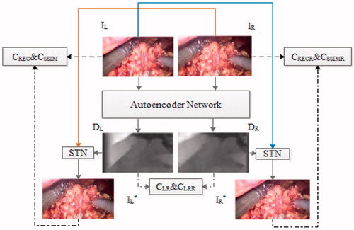
The auto-encoder network comprised two parts: encoder network and decoder network. The encoder network was inspired by the methods described in previous studies [11–13]. The deeper bottleneck architectures [14] were adopted for the Resnet101 encoder network, and the last layer of the fully connected layer was removed to reduce the number of parameters. The encoding network architecture is summarized in Table 1. The architecture with multiscale and skip plus [15] was used in the decoder network part. The method discussed in previous studies [6, 9] was used in the disparity acquisition layer. The sigmoid activation function was used in the convolution layer to obtain the depth image.

Table 1. Encoder and decoder part.

Encoder (Resnet101)
Layer		In/Out/K/S	Number	Output size
Conv1		3/64/7/2	1	128 × 64
Pool		–/–/3/2	1	64 × 32
Conv2_x	Conv2_1	64/64/1/1	3	32 × 16
	Conv2_2	64/64/3/–
	Conv2_3	64/256/1/1
Conv3_x	Conv3_1	256/128/1/1	4	16 × 8
	Conv3_2	128/128/1/–
	Conv3_3	128/512/1/1
Conv4_x	Conv4_1	512/256/1/1	23	8 × 4
	Conv4_2	256/256/3/–
	Conv4_3	256/1024/1/1
Conv5_x	Conv5_1	1024/512/1/1	3	4 × 2
	Conv5_2	512/512/3/–
	Conv5_3	512/2048/1/1
		Decoder
	Layer		In/Out/K/S	Output size
DeConv6_x	DeConv5_3		2048/512/3/2	8 × 4
	Plus6	DeConv5_3 + Conv4_3	–/1536/–/–
	Conv6	Plus6	1536/512/3/1
DeConv5_x	DeConv6		1024/256/3/2	16 × 8
	Plus5	DeConv6 + Conv3_3	–/768/–/–
	Conv5	Plus5	768/256/3/1
DeConv4_x	DeConv5		512/128/3/2	32 × 16
	Plus4	DeConv5 + Conv2_3	–/384/–/–
	Conv4	Plus4	384/128/3/1
	Disp4	Conv4
DeConv3_x	DeConv4		128/64/3/2	64 × 32
	Plus3	DeConv4 + pool + Disp4*	–/130/–/–
	Conv3	Plus3	130/64/3/1
	Disp3	Conv3
DeConv2_x	DeConv3		96/32/3/2	128 × 64
	Plus2	DeConv3 + Conv1 + Disp3*	–/98/–/–
	Conv2	Plus2	98/32/3/1
	Disp2	Conv2
DeConv1_x	DeConv2		32/16/3/2	256 × 128
	Plus1	DeConv2 + Disp2*	16/18/–/–
	Conv1	Plus1	18/16/3/1
	Disp1	Conv1

Conv, Convolution; pool, max pooling; Conv _x, convolution blocks; DeConv, deconvolution; DeConv _x, deconvolution block; Disp, disparity layer; In, input channels; K, kernel size; Number, block number; Out, output channels; Output size, output image size; Plus, skip connection; S, stride; *, upsampling factor 2.

2.2. Binocular depth estimation loss function

The loss function was minimized to train the unsupervised binocular depth estimation network. The loss function included three parts. The first part was the left–right consistency loss of the error calculated by the L1 metric C_LR between the predicted left disparity D_L and right disparity D_R, where (i, j) is the pixel index of the image: (1) $$C_{LR}=\frac{1}{N}{\displaystyle {\sum }_{i,j}\left(|D_L(i,j)-D_R(i+D_L(i,j),j)|\right)}$$(1)

The second part was the structural similarity loss C_SSIM (where SSIM is the structural similarity index) of the error between the input image and the reconstruction image (the right counterpart is C_SSIMR) (2) $$C_{\mathit{\text{SSIM}}}=\frac{1}{N}{\sum }_{i,j}\frac{2}{5}\left(|1-\mathit{\text{SSIM}}(I_L(i,j),I_L^{*}(i,j)\left)\right|\right)$$(2)

The third part was the reconstruction error loss between the input image I_L(i,j) and the reconstruction image I_L*(i, j) (the right counterpart isC_RECR): (3) $$C_{REC}=\frac{1}{N}{\displaystyle {\sum }_{i,j}\left(|I_L(i,j)-I_L^{*}(i,j)|\right)}$$(3)

Four layers of loss function occurred at different scales, and the scale factor was 2. The total loss function was as follows, and α = β = λ = 1. (4) $$C={\sum }_{s=1}^4\left(\alpha \left(C_{LR}+C_{LRR}\right)+\beta \left(C_{REC}+C_{\mathit{\text{RECR}}}\right)+\lambda \left(C_{\mathit{\text{SSIM}}}+C_{\mathit{\text{SSIMR}}}\right)\right)$$(4)

2.3. Training details

An unsupervised binocular depth estimation method was implemented using the TensorFlow framework on Nvidia Tesla P100 GPU (16 GB). An exponential activation function was used in each convolution and deconvolution except for convolution to obtain the disparity map. The Adam optimizer was used. The network had 50 epochs on the training datasets, and the initial learning rate was set to 10^-4. The batch sizes were 16, and the total training time was about 8 h. The images were resized to 256 × 128 to reduce the computational time. The number of parameters was about 9.5 × 10⁷.

3. Results

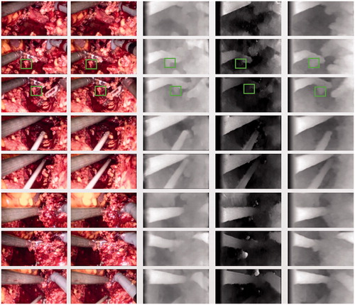
The unsupervised binocular Resnet network depth estimation method was compared with the basic [14] (unsupervised single convolutional neurla network CNN) and Siamese [14] (unsupervised binocular CNN) methods illustrated in Figure 2. The higher intensity meant that the distance to the camera was closer.

Figure 2. Example results of the three methods. The left two columns are the input images; the third column is the Siamese result; the fourth column is the Basic result; and the last column is the result of this study. Green boxes indicate comparisons of different results under the same organization.

No ground-truth result was available for the dataset. Therefore, the performance was compared with all published results, and the best results were taken as the ground-truth result for evaluation using SSIM and the peak signal-to-noise ratio (PSNR). The average evaluation value of the 7191 pairs of calibrated stereo images in the testing set was evaluated. The results are described in Table 2. The time for generating the predicted depth image was about 16 ms.

Table 2. Comparison of evaluation results between the basic and the methods used in this study.

Method	Basic	Present study
Mean SSIM	0.5414 ± 0.0709	0.8349 ± 0.0523
Mean PNSR	7.7650 ± 1.3686	14.4957 ± 1.9676

PSNR, Peak signal-to-noise ratio; SSIM, structural similarity index.

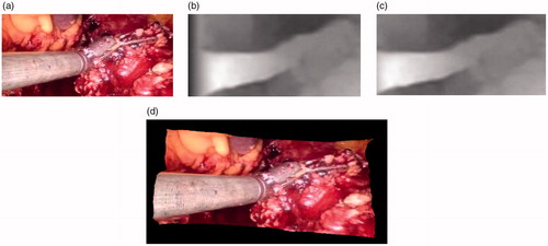
The 3D reconstruction was performed on the left image with the corresponding disparity map and the internal and external parameters of the left camera of the 3D laparoscopy. In the process of 3D reconstruction, an error appeared on the left side of the disparity map due to the occlusion of the laparoscopy, as shown in Figure 3(b). We cut the occluded part and the remaining part is shown in Figure 3(c), and the remaining part is reconstructed as shown in Figure 3(d).

Figure 3. An example of 3 D reconstruction. (a) Left image. (b) Disparity map. (c) Post-processing. (d) 3 D reconstruction.

4. Discussion

The results of the present study were found to be better than those obtained using basic methods and similar to those obtained using the Siamese method (Figure 2 and Table 2). For example, the green boxes in Figure 2 show a whole piece of prominent human tissue. The right half of the tissue is covered with blood, indicating that the tissue was at the same distance from the camera and had same brightness. The result correctly shows the depth map of the covered part.

In the 3D reconstruction in Figure 3, only pixels were mapped to color in the left image to spatial 3D coordinates, showing the correctness of the estimated depth values and the superiority of the 3D reconstruction results.

5. Conclusions

In this study, a novel end-to-end depth prediction network method was proposed for laparoscopic soft-tissue 3D reconstruction. The residual network was first used in the depth estimation of binocular laparoscopic soft-tissue surface to generate better dense prediction depth maps. The time to generate a map was only 16 ms, which could fulfill the real-time display requirements of real surgical scenes because the calculation of the depth images was the most time-consuming part of the 3D reconstruction.

The future studies would train abdominal soft-tissue surface depth estimation networks through transfer learning and ensemble learning with fine-tuning, enhancing the robustness and accuracy further.

Additional information

Funding

This study was supported by the National Key Research and Development Program [Nos. 2016YFC0106500/2 and SQ2017ZY040217/03], the NSFC-Guangdong Union Grant [No. U1401254], the NSFC-Shenzhen Union Grant [No. U1613221], the Guangdong Scientific and Technology Program [No. 2015B020214005], the Shenzhen Key Basic Science Program [No. JCYJ20170413162213765], and the Shenzhen Key Laboratory Project under Grant ZDSYS201707271637577.