Real-time tracking of surgical instruments based on spatio-temporal context and deep learning

ABSTARCT

Real-time tool tracking in minimally invasive-surgery (MIS) has numerous applications for computer-assisted interventions (CAIs). Visual tracking approaches are a promising solution to real-time surgical tool tracking, however, many approaches may fail to complete tracking when the tracker suffers from issues such as motion blur, adverse lighting, specular reflections, shadows, and occlusions. We propose an automatic real-time method for two-dimensional tool detection and tracking based on a spatial transformer network (STN) and spatio-temporal context (STC). Our method exploits both the ability of a convolutional neural network (CNN) with an in-house trained STN and STC to accurately locate the tool at high speed. Then we compared our method experimentally with other four general of CAIs’ visual tracking methods using eight existing online and in-house datasets, covering both in vivo abdominal, cardiac and retinal clinical cases in which different surgical instruments were employed. The experiments demonstrate that our method achieved great performance with respect to the accuracy and the speed. It can track a surgical tool without labels in real time in the most challenging of cases, with an accuracy that is equal to and sometimes surpasses most state-of-the-art tracking algorithms. Further improvements to our method will focus on conditions of occlusion and multi-instruments.

Keywords:

• Tool tracking
• convolutional neural network
• spatial transformer network
• spatio-temporal context

Introduction

Detection and tracking of surgical instruments are crucial to computer-assisted interventions (CAIs) for minimally-invasive surgery (MIS) [1]. Recently, CAIs for MIS have attracted increasing attention, since they offer several advantages over traditional MIS. They can improve the accuracy of the location of surgical tools, enhance the control capabilities of the surgeons performing the procedures, and reduce the cost of human assistants; collectively, these advantages make surgery more efficient. CAI techniques can be divided into two categories: hardware-based and image-based solutions. Hardware-based solutions require modification to instrument design, which poses ergonomic challenges and additionally suffers from robustness issues due to line-of-sight requirements [2]. Therefore more and more CAI techniques are using image-based solutions. Most image-based solutions employ visual tracking algorithms, since CAI systems are endoscopically controlled to automatically track the instruments.

The difficulties in tracking surgical instruments, such as motion blur, adverse lighting conditions, specular reflections on the tool surfaces and on the tissue regions, and shadows cast by the tool, can lead to inaccuracy [3]. Certain instruments that employ robot kinematic information from joint encoders to track the movements of an entire surgical instrument [4] are typically fast and robust, since they can recover when the instruments are occluded by tissue, smoke or shadows from other instruments, however, the accumulation of errors can result in a significantly large aggregate error [5]. The method of extracting image features with gradients [6] can accurately render partial surgical tool features, however, it has two disadvantages: one being that gradients are sensitive to noise, illumination and shadows [7], while the other is that the gradient distribution rate is difficult to obtain [8]. In addition, the methods of template matching by learning [9,10], can accurately extract features from image patches and quickly and robustly track the instruments, since they use a paradigm of pre-training to carry out image matching. This paradigm or template can be enhanced by learning with random forests (RFs) [11], gradient descents and filters, however, these methods lack a large amount of data with which to train the paradigm. They are valid on certain surgical instruments under certain conditions, but cannot deal well with the above-mentioned difficulties. Recently, the CNNs have a great performance on visual tracking [12–14] as the excellent target identification ability of the CNNs.

In the present paper, therefore, we propose a visual tracking approach using a CNN with a spatial transformer network (STN) for the location-determination process and a spatio-temporal context learning algorithm (STC) [15] for the process of tracking frame by frame. Developments in stereo cameras [16] make the achievement of three-dimensional (3D) reconstruction easier, thus, we can focus on the 2D positions of surgical tools in a single image using a CNN. We can subsequently utilize the information between contiguous frames to quickly and consistently execute tracking. During robotic surgery, surgeons tend to work very close to the anatomy, and most prior work that emphasizes the shaft of the robotic instrument work relatively poorly. Therefore, our present work emphasizes the tip of the tools, supplemented by the detection of the shaft. Our contribution is improving a CNN accompanied by an STN [17], and use a network that was trained by new and existing datasets to locate the tip in a single image. Following detection, we utilize the STC to track the tip between frames. Instead of detection by tracking, our algorithm’s mode is simultaneous detection and tracking, which benefits both speed and accuracy. Subsequently, we discriminatively utilize our method and other methods in a series of video frames, showing that our method is equal to or exceeds state-of-the-art surgical instrument tracking.

Method

As mentioned above, our method is based on classification by a CNN and tracking by an STC. In this section, we describe how the CNN detects the tool’s tip and how the STC tracks the tool between frames in real time.

A spatial transformer network within a convolutional neural network

With the development of computer hardware, modern computers can store very large amounts of data, thus, we can apply tool detection to deep neural networks. As one type of deep neural networks, a CNN can extract image features faster and more efficiently than other types. There are also several benefits to using a CNN compared with other state-of-the-art machine-learning approaches. Firstly, the features extracted by a CNN are unknown, complex and effective, instead of simple corner features, edge detection, colour tags and other classic and hand-crafted features [18]. Therefore, a CNN is not only free from the disadvantages of hand-crafted features, but it also eliminates errors from hand-crafted features and reduces errors from simple features. We only need to use image datasets to train a CNN, without pre-processing, to accurately detect a tool. Furthermore, during surgical tool tracking, a CNN can be pre-trained using a database containing a large number of specific surgical tools, and fine-tuned with additional domain-specific images [3], which can include the challenging conditions mentioned above, so that CNNs can manage them.

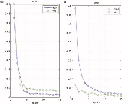
To better manage the challenges of the spatial positions of a tool, we introduce an STN as the location network within our network structure. The STN can manage the translation, rotation, scale and increased generic warping [18] of the tool without an increased cost of time, which augments the accuracy of classification and overcomes over-fitting. According to [18], in a noisy environment, on $60\times 60$ images with translated MNIST digits and background clutter, a CNN gets 3.5% error, while a CNN with the STN gets 1.7% error. In addition, we test our model using one of our own datasets, as shown in Figure 1, our network without the STN gets 3.9% error (validation error), while our network with the STN gets 0.7% error (validation error).

Figure 1. The training and validation error of the CNN, (a) our network without the STN; (b) our network with the STN.

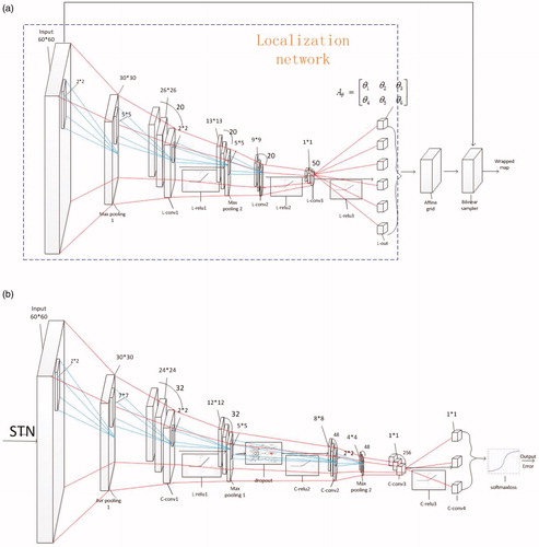
In our structure, as shown in Figure 2(a), the STN localization network has nine layers, consisting of three convolutional layers, followed by rectified linear units (ReLU) as an activation function, as the ReLU makes the stochastic gradient descent (SGD) converge faster than the sigmoid and the tanh function, and two max-pooling layers in front of the first two convolutional layers to down-sample the input. Additionally, differing from the classification network, the final layer of the localization network is a convolutional regression layer. The localization network can produce six affine transformation parameters [17] through back-propagation. Subsequently, the next two layers are the affine grid and bilinear sampler layers. Specifically, an affine transformation is applied to a mesh grid to produce an image that determines how points are selected from the input, which is mapped back onto the grid. The next step is to run a bilinear interpolation sampler on the grid to obtain the output of the STN. The affine transformation allows zooming, rotation and skewing of the input, as shown in equation (1)(1) $$A_{\theta }=\left[\begin{array}{ccc}{\theta }_1& {\theta }_2& {\theta }_3\\ {\theta }_4& {\theta }_5& {\theta }_6\end{array}\right]$$(1) : (1) $$A_{\theta }=\left[\begin{array}{ccc}{\theta }_1& {\theta }_2& {\theta }_3\\ {\theta }_4& {\theta }_5& {\theta }_6\end{array}\right]$$(1)

Figure 2. Specific network architecture of (a) the STN and (b) the classification network.

Where ${\theta }_1$ and ${\theta }_5$ are the zooming parameters, ${\theta }_2$ and ${\theta }_4$ are the rotation parameters, ${\theta }_3$ and ${\theta }_6$ are the skewing parameters. Through the STN, we can obtain the adjusted map as the input for the classification network, which comprises the other layers of the CNN. The specific network architecture is shown in Figure 2.

As shown in Figure 2(b), the classification network has 13 layers, consisting of three convolutional layers, followed by a ReLU, a final convolutional layer, a softmax-loss layer which combines a softmax layer (the classification layer) and a multinomial logistic loss layer to reduce the computational complexity. We set the size of the convolutional kernels as $7\times 7$, $5\times 5$, $4\times 4$ and $1\times 1$ to produce one score for three kernels combined with pooling layers, and the pooling layers comprise both the average-pooling and the max-pooling to decrease the errors and redundancy of the feature. However, there is a problem of over-fitting due to the small size of our training sample, which should be solved, therefore, we added dropout layers to the structure, as demonstrated in [19], which can prevent over-fitting of the model. Differing from the situation described in [20] we use an in-house dataset to train a specialized CNN for surgical tool tracking.

The output of the last convolutional layer has three labels, namely tip, shaft and background. By repeatedly scanning the input image with a fixed sliding window (for simplicity, accuracy and speediness, we set the size of the window as the sizes of the training image patches. During the network training, we manually take a set of patches where the tip is far from the camera as the training patches, and the size of these patches is the same as other training patches, thus, our detector can deal with conditions where the scale of the tool is too small. If the tip is too close to the camera, our detector cannot detect the tip, however, it can output a position that is the most similar to the tip until the scale of the tip become regular, nevertheless, this did not happen in our datasets). We can place these patches into our classification network to estimate its category, which can locate the shaft part, and then take advantage of the linear relevance between the shaft and the tip to find the likely location of the tool tip (firstly, we locate 10 shaft patches and estimate a linear relevance path between the shaft and the tip, then we can find the possible tip locations by only inputting the patches central on the line with three types of stride, which needs little time). Subsequently, we can find the best location of the tip in the surroundings of possible locations, which is our detection algorithm.

Real-time tracking by spatio-temporal context learning

The drawback of the CNN and STN that we use is that it cannot track the object in real time. The average time of solely using the neural network to detect the tip of the surgical tool in one frame is approximately 2.5 s for a $720\times 480$ RGB image on an i3 CPU, however, this computational time is well below the frame rate of endoscopic video, which is generally 25, 30 or 60 frames per second (fps) [14] Therefore, we cannot use the strategy of tracking by detection.

The strategy employed here, therefore, is to capture the spatio-temporal context information of the tip location between two frames using an STC learning algorithm [15], which can overcome the above problem. This algorithm adopts a fast Fourier transform (FFT) and the context information, and, implementing this algorithm in MATLAB without code optimization, the proposed tracker runs at 350 fps on an i7 machine [15] and at 48 fps on our i3 machine, which is up to the real-time standard. However, this approach needs a manual location and lacks the mechanism of repeated location when the tracker cannot track the object. Thus, we improve this approach and combine it with the detection algorithm to achieve fully-automatic operation and to find the object that is being tracked when it is lost. Although our method also tracks the tool in one extended area, it detects the object in the entire image if it cannot track the tool successfully, thus, it can also track the tool when the tool moves too fast. This process is shown in Figure 3 and is called repeated location.

Figure 3. (a) Learning spatial context at the $t_{th}$ frame; (b) detecting an object’s location at the ${(t+1)}_{th}$ frame and tracking.

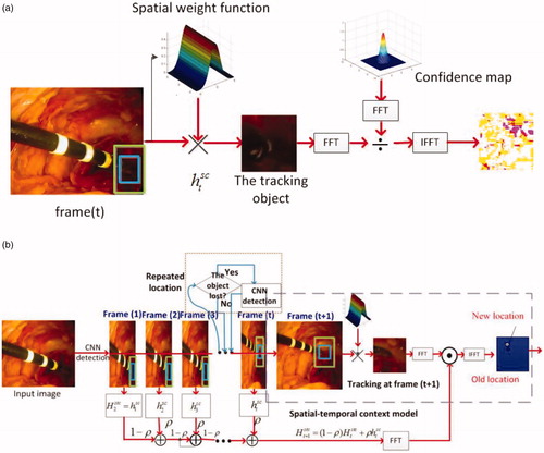
Our tracking and detection process is illustrated in Figure 3. Firstly, we use the CNN with an STN to locate the tip of the tool in the entire image, instead of using manual location. The STC learning algorithm then formulates spatio-temporal relationships between the location of the tip and its local context based on a Bayesian framework, according to these equations we can obtain the statistical correlation model of the low-level features between the target and its surrounding regions. Simultaneously, repeated relocation occurs when the scale of the rectangular window is overly large or undersized, or if the position of the tracker does not move for several frames (empirically, five frames). During this process, according to the following equations, it can compute the confidence map ($c(x)$) according to the spatial context prior probability $I(z){\omega }_{\sigma }(z-x^{*})$ and the conditional probability ($h^{sc}(x-z)$) of the latest continuous frames (equation (2)(2) $$c\left(X\right)=b{e}^{-{\left|\frac{x-x^{*}}{\alpha }\right|}^{\beta }}=\sum _{z\in {\Omega }_c\left(x^{*}\right)}{h}^{sc}(x-z)I\left(z\right){\omega }_{\sigma }(z-x^{*})$$(2) ); and then takes the maximal value of the new confidence map ($c_{t+1}(x)$) of the next frame to obtain the new object location ($x_{t+1}^{*}$) in the next frame (equation (3)(3) $$x_{t+1}^{*}=\underset{x\in {\Omega }_c\left(x_t^{*}\right)}{\arg \max }{c}_{t+1}\left(x\right)$$(3) ). To compute the new confidence map ($c_{t+1}(x)$), it needs to update the spatio-temporal context model ($H_{t+1}^{stc}$) (equation (4)(4) $$H_{t+1}^{stc}=(1-\rho )H_t^{stc}+\rho h_t^{sc}$$(4) ), taking the temporal Fourier transform of the spatio-temporal context model ($H_{t+1}^{stc}$) and the temporal Fourier transform of the spatial context prior probability in the next frame ($I_{t+1}(z){\omega }_{\sigma }(z-x^{*})$) into equation (2)(2) $$c\left(X\right)=b{e}^{-{\left|\frac{x-x^{*}}{\alpha }\right|}^{\beta }}=\sum _{z\in {\Omega }_c\left(x^{*}\right)}{h}^{sc}(x-z)I\left(z\right){\omega }_{\sigma }(z-x^{*})$$(2) . We can obtain the new confidence map ($c_{t+1}(x)$) by inverse FFT function of the equation (2)(2) $$c\left(X\right)=b{e}^{-{\left|\frac{x-x^{*}}{\alpha }\right|}^{\beta }}=\sum _{z\in {\Omega }_c\left(x^{*}\right)}{h}^{sc}(x-z)I\left(z\right){\omega }_{\sigma }(z-x^{*})$$(2) . Finally, the estimated scale of the window ($s_{t+1}$) is updated by the estimated scale between two consecutive frames ($s_t^{\prime }$), the average of the estimated scales from n consecutive frames (${\overline{s}}_t$) and a fixed filter parameter ($\lambda$) similar to the learning rate (here set to 0.075) (equation (5)(5) $$\{\begin{array}{c}{s}_t^{\prime }=\sqrt{\frac{c_t\left({\mathbf{x}}_{\mathbf{t}}^{*}\right)}{{\mathbf{c}}_{\mathbf{t}-\mathbf{1}}\left({\mathbf{x}}_{\mathbf{t}-\mathbf{1}}^{*}\right)}}\\ {\overline{s}}_t=\frac{1}{n}{\sum }_{i=1}^n{s}_{t-i}^{\prime }\\ s_{t+1}=(1-\lambda )s_t+\lambda {\overline{s}}_t\\ {\sigma }_{t+1}=s_t{\sigma }_t\end{array}$$(5) ). The main functions are as follows: (2) $$c\left(X\right)=b{e}^{-{\left|\frac{x-x^{*}}{\alpha }\right|}^{\beta }}=\sum _{z\in {\Omega }_c\left(x^{*}\right)}{h}^{sc}(x-z)I\left(z\right){\omega }_{\sigma }(z-x^{*})$$(2) (3) $$x_{t+1}^{*}=\underset{x\in {\Omega }_c\left(x_t^{*}\right)}{\arg \max }{c}_{t+1}\left(x\right)$$(3) (4) $$H_{t+1}^{stc}=(1-\rho )H_t^{stc}+\rho h_t^{sc}$$(4) (5) $$\{\begin{array}{c}{s}_t^{\prime }=\sqrt{\frac{c_t\left({\mathbf{x}}_{\mathbf{t}}^{*}\right)}{{\mathbf{c}}_{\mathbf{t}-\mathbf{1}}\left({\mathbf{x}}_{\mathbf{t}-\mathbf{1}}^{*}\right)}}\\ {\overline{s}}_t=\frac{1}{n}{\sum }_{i=1}^n{s}_{t-i}^{\prime }\\ s_{t+1}=(1-\lambda )s_t+\lambda {\overline{s}}_t\\ {\sigma }_{t+1}=s_t{\sigma }_t\end{array}$$(5) Where $I(z)$ denotes the image intensity and $I_{t+1}(z)$ denotes the image intensity of the next frame, ${\omega }_{\sigma }(\cdot )$ is the weight function; $H$ denotes the time domain and $h$ denotes the spatial domain, $\rho$ is the learning parameter, and $h_t^{st}$ is the spatial context model; $n$ is the number of consecutive frames and $\sigma$ denotes the scale parameter.

Experiments and Results

To demonstrate the feasibility of the proposed methodology, we compared our method to four other methods using eight validation video datasets. For every experiment, this work used each single dataset to train a specific model, since it is easier to converge the model in its training process, and made the classification more accurate for one type of tool than for various types of tools. These datasets were from online and in-house surgical videos in a wide variety of surgical settings, which were divided into three categories, tip, shaft and background patches, for in vivo abdominal condition [21] (500 frames, 600 test patches, and 2100 training patches), laparoscopic simulation [22] (1439 frames, 600 test patches, and 2500 training patches), light-changing [23] (254 frames, 200 test patches, and 900 training patches), retinal [6] (222 frames, 200 test patches, and 1000 training patches), smoky [23] (267 frames, 200 test patches, and 1200 training patches), cardiac [11] (433 frames, 400 test patches, and 2100 training patches), standard dataset [1] (5261 frames, 800 test patches, and 4000 training patches), and our own simulation (1000 frames, 400 test patches, and 2100 training patches) conditions. The datasets also contained various challenges such as light changes, smoky conditions and motion blur. The ground truth of the datasets in [21] and [23] was obtained manually, while the retinal and cardiac datasets had the ground truth embedded in their files.

The other four methods that we chose were: correlation filter tracking with convolutional features (CF) [20] (the VGG Net was selected as the CNN model, and the weights for combining correlation filter responses were (1, 0.5, 0.2) in our experiments), data-driven visual tracking (DDVT) [6] (half the radius of the search window $\sigma$ was 25 and the learning rate was set to 0.85 in our experiments), tracking with an active testing filter (ATF) [10] (training set included 50 images and AT optimization is $256\times 256$ in our experiments), and tracking with online multiple instance learning (MIL) [22] (search radius was set to 25 pixels, the number of negative image patches random sampling was 65, positive radius $r=4$, learning rate was set to 0.85, candidate weak classifier $M$ was set to 250 and chosen weak classifier $K$ was set to 50 in our experiments).

We implement our method in MATLAB, without a GPU (Graphics Processing Unit). The results were generated using an i3 − 4160T CPU @ 3.10 GHz. All reported results were obtained using a CNN with an STN for each dataset. The test video images were obtained by implementing five methods on eight datasets, and are shown in Figure 4. The error curves based on the experiments are shown in Figure 5, the Y-axis denotes the error value and the X-axis denotes the sequence number of frame.

Figure 4. Test video images, from top to bottom, with rows showing the performance of our method, the MIL method, ATF method, DDVT method, and CF method on eight datasets, respectively. Every column represents one kind of dataset; the dataset names appear below each column.

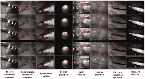
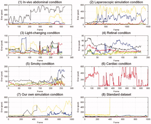
Figure 5. Each graph represents one kind of dataset and each colour line represents each method’s error; the dataset names appear below each graph. Red represents the error of our method, green that of the CF method, yellow that of the MIL method, black that of the ATF method, and blue that of the DDVT method.

The mean tracking errors in pixels (Euclidean distance between the tracking positions and the ground truth) are shown in Table 1, and if the error was larger than 150 pixels, we set it as N/A. The standard deviations (std) of the Euclidean distances are shown in Table 2, and if the std was larger than 150 pixels, we set it as N/A.

Table 1. Mean tracking errors (pixel) of every method on every dataset.

Dataset Algorithms	In vivo Abdominal condition	Laparoscopic simulation condition	Light- Changing condition	Retinal condition	Smoky condition	Cardiac condition	Our own simulation condition	Standard dataset
DDVT [6]	41.98	45.40	28.29	21.18	28.47	N/A	40.46	37.05
MIL [22]	N/A	N/A	45.71	9.02	32.08	N/A	N/A	N/A
CF [20]	14.40	13.47	25.64	10.45	18.98	N/A	35.21	39.43
ATF [10]	N/A	N/A	45.37	36.85	55.33	N/A	N/A	N/A
Ours	15.35	12.44	17.58	13.71	16.86	N/A	14.42	11.31

Table 2. Standard deviations (pixel) of every method’s tracking errors on every dataset.

Dataset Algorithms	In vivo Abdominal condition	Laparoscopic simulation condition	Light- Changing condition	Retinal condition	Smoky condition	Cardiac condition	Our own simulation condition	Standard dataset
DDVT [6]	21.77	70.50	27.61	17.22	12.26	N/A	52.04	64.77
MIL [22]	N/A	N/A	22.27	3.98	13.91	N/A	N/A	N/A
CF [20]	8.17	7.61	17.42	5.32	7.95	N/A	4.18	8.55
ATF [10]	N/A	N/A	22.38	12.41	17.06	N/A	N/A	N/A
Ours	13.67	19.14	20.52	6.81	9.97	N/A	2.63	9.42

Since the strategy for our method was tracking and detection, we needed certain frames to justify whether the tracker lost the tip and needed relocating if the tip was lost, thus, the tip may have been lost in several continuous frames. The accuracy of our method and each dataset are shown in Table 3. Frames per second (FPS) is another significant measurement that can show whether one algorithm is real time. The FPS for every method on every dataset is shown in Table 4 (N/A means this algorithm cannot track the tool in most frames).

Table 3. The trackers’ accuracy on every dataset; the accuracy have been calculated based on the distance between the ground truth and the tracking position. If the distance is smaller than the half length of side of the tracking window centred on the ground truth in one frame, we believe the tracker successfully track the object in this frame.

Dataset Algorithms	In vivo Abdominal condition	Laparoscopic simulation condition	Light- Changing condition	Retinal condition	Smoky condition	Cardiac condition	Our own simulation condition	Standard dataset
DDVT [6]	87%	89%	90%	90%	98%	5%	94%	99%
MIL [22]	74%	17%	73%	100%	40%	5%	40%	96%
CF [20]	96%	99%	96%	100%	100%	9%	99%	100%
ATF [10]	10%	35%	88%	95%	23%	5%	22%	79%
Ours	93%	96%	99%	100%	100%	82%	100%	100%

Table 4. Every method’s frames per second (FPS) on every dataset.

Dataset Algorithms	In vivo Abdominal condition	Laparoscopic simulation condition	Light- Changing condition	Retinal condition	Smoky condition	Cardiac condition	Our own simulation condition	Standard dataset
DDVT [6]	0.61	0.57	0.60	0.60	0.60	N/A	0.63	0.62
MIL [22]	0.19	0.26	0.27	0.22	0.26	N/A	0.26	0.21
CF [20]	0.64	0.72	0.64	0.61	0.67	N/A	1.59	1.34
ATF [10]	N/A	2.64	4.54	1.80	2.76	N/A	2.15	2.40
Ours	33.19	37.89	34.25	32.41	40.58	5.20	35.61	25.10

Discussion

Every condition under which we performed experiments had various challenges, except for that illustrated above. For instance, in the in vivo abdominal scenario, the tool moved quickly and widely, sometimes the tip moved out of view, and sometimes tissue adhered to the tip. In the cardiac scenario, the tool moved faster than in the abdominal scenario, and sometimes the tracker lost its object for several frames. We then chose the simulation conditions to compare with the in vivo case, and chose the retinal condition to test the performance of our model in other environments. Therefore, according to the results shown in Figure 5 and Tables 1 and 2, we can conclude that the performance of these methods was different under different conditions.

Performance on the accuracy

In terms of accuracy, our method performed as well as the CF method (the std of our method was a little larger than that of the CF) and better than the three other methods on most datasets (the retinal condition is a basic condition that has no challenges, and we used it to validate whether every method could track the tool successfully under simple conditions. It can be seen in Figure 5 that its degree of difficulty was lower than that of the other conditions, thus, all methods could perform well and there were only small differences between their accuracy). The ATF and MIL methods could not track the tip from certain frames to the end, especially when the tool moved quickly and over a wide area. The tracking accuracy of the DDVT method was in the middle, but its speed was very slow. In the cardiac condition, the CF method could not successfully track the tip, since the strategy of this algorithm is tracking by detection, and it detects the object in the extended area around the tracking window to increase tracking speed, but the tool moves too fast in the cardiac condition to be found in its extended area. From another point of view, the CF method also uses the CNN, which demonstrates that a method using a CNN would exhibit high accuracy. The results presented in Table 3 show that the accuracy of our method was able to meet the tracking requirements, and that our method could manage most of the challenges, however, if the tool moved too fast or too frequently in and out of view, the tracking dropped certain frames and began the relocation operation by the CNN, the process of which was explained above. In the cardiac condition, there were more dropped frames than in any other condition, which led to a reduction in accuracy.

Performance on the speed

In terms of speed, repeated location operations occurred more times in the cardiac condition than in any other condition, which led to an increase in tracking time, as shown in Table 4. According to the results presented in Table 4, our method was equal in terms of real-time performance in most cases, and was faster than other methods even in the cardiac condition. The CF method had high accuracy, but sacrificed the tracking speed to some extent, while the ATF method was slightly faster than the other three methods, but its accuracy was too low. From Table 4, the FPS of our method in the standard dataset was lower than in the other conditions, since the image size of the standard dataset ($1920\times 1080$) was larger than in the other conditions. When our method repeated the location of the tip, it took more time to manage the entire input image. Based on the experiments’ results shown in Figure 5 and Table 1, we can see that the MIL method could only track the tool successfully in former frames, and its FPS achieved in the standard dataset was less than that in other conditions, since the MIL method saved the information of all the former frames, which consumed so much memory that the process ran for a long time, and the larger the image, the fewer frames it could process. However, our tracking strategy only used the information from the latest three to five frames, which resulted in not only a high speed, but also a high accuracy.

Conclusion

Visual tracking using a CNN with an STN and an STC has been highlighted as an extremely promising algorithm for MIS images. In most cases, it can track a surgical tool without labels in real time with an accuracy that is equal to and sometimes surpasses most state-of-the-art general or CAIs’ visual tracking algorithms. Furthermore, it does not need manual location in the first frame. However, the results of the cardiac condition show that our method has shortcomings. Firstly, the re-location operation by the CNN took a long time over the entire tracking process, and secondly, the relocation operation increased the number of failing frames. Therefore, our future work will include decreasing the detection time by the use of, for example, GPU to accelerate the classification process of the CNN, enlarging the training dataset and using the batch normalization method to prevent over-fitting in order to increase the precision location determination, and improving the relocation process to find the failing frames in time. Moreover, we will use the thoughts in the YOLO [24] and region proposal networks to shorten the detection and relocation time. Thus, we should improve the accuracy and FPS of our method, in particular under conditions of occlusion and multi-instruments.

Acknowledgments

The authors would like to thank TIMC-IMAG for supplying the ex-vivo and in-vivo laparoscope data.

Disclosure statement

No potential conflict of interest was reported by the authors.

Additional information

Funding

This work has been supported by the Specialized Research Fund for the Doctoral Program of Higher Education of China (No.20130131120036), the Promotive Research Fund for Excellent Young and Middle-aged Scientists of Shandong Province (No.BS2013DX027), the National Natural Science Foundation of China (No.81401543, 61673244), the French National Research Agency (ANR) through TecSan Program.

References

- Du X, Maximilian A, Alessio D, et al. Combined 2D and 3D tracking of surgical instruments for minimally invasive and robotic assisted surgery. Int J Comp Assisted Radiol and Surg. 2016;11(6):1109–1119.
- Austin R, Peter KA, Zhao T. Feature classification for tracking articulated surgical tools. Proceedings of the 15th International Conference on Medical Image Computing and Computer-Assisted Intervention-MICCAI; 2012 Oct 1–5; Nice, France. p. 592–600.
- Wesierski D, Wojdyga G, Jezierska A. Instrument tracking with rigid part mixtures model. Proceedings of the International Workshop on Computer-Assisted and Robotic Endoscopy; 2015 Oct; Munich. p. 22–34.
- Felzenszwalb PF, Girshick RB, McAllester D, et al. Object detection with discriminatively trained part-based models. IEEE transac pattern anal machine intel. 2010;32(9):1627–1645.
- Reiter A, Allen PK, Zhao T. Appearance learning for 3D tracking of robotic surgical tools. The Int J Robot Res. 2014;33(2):342–356.
- Sznitman R, Ali K, Richa R, et al. Data-driven visual tracking in retinal microsurgery. Proceedings of the 15th International Conference on Medical Image Computing and Computer-Assisted Intervention-MICCAI; 2012 Oct 1–5; Nice, France. p. 568–575.
- Agustinos A, Voros S. 2D/3D real-time tracking of surgical instruments based on endoscopic image processing. Proceedings of the International Workshop on Computer-Assisted and Robotic Endoscopy; 2015 Oct; Munich. p. 90–100.
- Allan M, Chang P, Ourselin S, et al. Image based surgical instrument pose estimation with multi-class labelling and optical flow. Proceedings of the International Workshop on Computer-Assisted and Robotic Endoscopy; 2015 Oct; Munich. p. 331–338.
- Reiter A, Allen P K. An online learning approach to in-vivo tracking using synergistic features. Proceedings of IEEE/RSJ International Conference on Intelligent Robots and Systems (IROS); 2010 Oct 18–22; Taipei. p. 3441–3446.
- Sznitman R, Richa R, Taylor RH, et al. Unified detection and tracking of instruments during retinal microsurgery. IEEE transac patt anal machine intel. 2013;35(5):1263–1273.
- Sznitman R, Becker C, Fua P. Fast part-based classification for instrument detection in minimally invasive surgery. Proceedings of International Conference on Medical Image Computing and Computer-Assisted Intervention-MICCAI. 2014 Sept 17; Boston. p. 692–699.
- Liu Q, Lu X, He Z, et al. Deep convolutional neural networks for thermal infrared object tracking. Knowledge-Based Sys. 2017;134:189–198.
- Yang W, Zhou Q, Fan Y, et al. Deep context convolutional neural networks for semantic segmentation. Proceedings of CCF Chinese Conference on Computer Vision; 2017 Oct; Tianjin. p. 696–704.
- Nam H, Han B. Learning multi-domain convolutional neural networks for visual tracking. In: IEEE Conference on Computer Vision and Pattern Recognition; 2016 Jun 26–Jul 1; Las Vegas. p. 4293–4302.
- Zhang K, Zhang L, Yang M, et al. Fast tracking via spatio-temporal context learning. In arXiv: 1311.1939, 2013.
- Wang C, Palomar R, Cheikh FA. Stereo video analysis for instrument tracking in image-guide surgery. Proceedings of the 5th European Workshop on Visual Information Processing (EUVIP); 2014 Dec 10–12; Paris. p. 1–6.
- Jaderberg M, Simonyan K, Zisserman A. Spatial transformer networks. Adv in Neu Info Proc Sys. 2015;28:2017–2025.
- Garcia L, Li W,Gruijthuijsen C, et al. Real-time segmentation of non-rigid surgical tools based on deep learning and tracking. Proceedings of the International Workshop on Computer-Assisted and Robotic Endoscopy; 2016 Oct; Athens. p. 84–95.
- Hinton GE, Srivastava N, Krizhevsky A, et al. Improving neural networks by preventing co-adaptation of feature detectors. In arXiv: 1207.0580, 2012.
- Ma C, Huang J, Yang X, Yang M. Hierarchical convolutional features for visual tracking. Proceedings of the International Conference on Computer Vision; 2015 Dec 7–13; Santiago. p. 3074–3082.
- Zhao Z. Real-time 3D visual tracking of laparoscopic instruments for robotized endoscope holder. Bio-medical mat and eng. 2014;24(6):2665–2672.
- Babenko B, Yang M, Belongie S. Robust object tracking with online multiple instance learning. IEEE Transact patt anal and machine intel. 2011;33(8):1619–1632.
- Giannarou S, Visentini-Scarzanella M, Yang G. Probabilistic tracking of affineinvariant anisotropic regions. IEEE Transact patt anal and machine intel. 2013;35(1):130–143.
- Joseph R, Santosh D, Ross G. et al. You only look once: unified, real-time object detection. Proceedings of the IEEE Conference on Computer Vision and Pattern Recognition; 2016 Jun 26–Jul 1; Las Vegas. p. 779–788.