A novel technique for analysing histogram equalized medical images using superpixels

Abstract

We present a novel technique to distinguish between an original image and its histogram equalized version. Histogram equalization and superpixel segmentation such as SLIC (simple linear iterative clustering) are very popular image processing tools. Based on these two concepts, we introduce a method for finding whether an image (grayscale) is histogram equalized or not. Because sometimes we see images that look visually similar but they are actually processed or changed by some image enhancement process such as histogram equalization. We can merely infer whether the image is dark, bright or has a small dynamic range. Moreover, we also compare the result of SLIC superpixels with three other superpixel segmentation algorithms namely, quick shift, watersheds, and Felzenszwalb’s segmentation algorithm

Keywords:

• SLIC
• Superpixel
• Quick shift
• Watersheds
• Felzenszwalb
• AHE
• CLAHE

1. Introduction

Histogram equalization is an image enhancement method used in image processing. Histogram equalization techniques are used for contrast enhancement in a wide range of image types ranging from general, medical to satellite images. There are numerous variations of histogram equalization but in essence, they are divided into global and local histogram equalization. The algorithm proposed in [1] uses Gaussian Mixture Model to model the gray level distribution of images. Moreover, the intersection points of the Gaussian model are used to model the dynamic range of the images into input gray level intervals. Eunsung Lee et al. [2] proposed a method to compute brightness-adaptive intensity transfer functions by using the low-frequency luminance component in the wavelet domain and transforms intensity values according to the transfer function.

Automatic transformation is a method that improves the brightness of dim images via the gamma correction and probability distribution of luminance pixels. It also works very well for videos [3]. Segmentation algorithms are widely used for the segmentation of medical images [4], proposed a method for the medical image segmentation using watershed algorithms. Moreover [5], describes a method based on the histogram approach, for the enhancement of medical images using Gaussian Mixture Modeling GMM. Chen et al. [6] used SLIC superpixels to eliminate the effect of constructed defects and noise by means of the feature similarity in the preprocessing stage.

Medical image analysis is a broad field and provides a forum for a lot of research in the medical and biological research areas. There are different techniques available for the analysis of medical images. Machine learning (ML) approaches are successful in image-based diagnosis, disease prognosis, and risk assessment, such as Machine Learning for medical image analysis [7], the semiotics of image segmentation [8] and machine learning approaches in medical image analysis from detection to diagnosis [9]. E. Goceri et al. [10] have done a comprehensive survey on recent advances and future trends of Deep Learning (DL) in medical image analysis and stated that segmentation is the most common technique applied in medical image analysis using deep learning. Moreover [11], has discussed state-of-the-art methods for brain tissue segmentation like manual, region-based, thresholding-based, clustering-based, and feature extraction methods. A comprehensive review is done by [12] about the medical image segmentation on GPUs (Graphical Processing Unit). The image processing and visualization time are greatly reduced by using GPU platforms.

In this paper, firstly, we make use of two techniques to equalize the histograms of low contrast grayscale images and then we use four superpixel algorithms to segment the histogram-equalized images into superpixels. Finally, we extract the superpixel segments of the equalized images using four segmentation algorithms and compare the results. Our results show that SLIC superpixels are compact, grid-shaped and equal to the k number of superpixels that we extracted before the histogram equalization. We have tested grayscale medical images for experiments. Figure 1 shows the original image, two histogram equalized images, and histograms of each image. The flowchart of the proposed method is shown in Figure 2. Where GHE and CLAHE stands for Global Histogram Equalization and Contrast Limited Adaptive Histogram Equalization respectively. Moreover, Figure 3 illustrates the superpixels of original images as well as a comparison between the superpixels generated before and after histogram equalization. Subsequent sections of this paper contain a discussion of the histogram equalization techniques in section 2, a brief introduction of superpixel segmentation algorithms in section 3, our proposed technique in section 4, comparison of the results of segmentation is shown in section 5 and finally, section 6 concludes the paper.

Figure 1. Original image, global histogram equalized image, CLAHE equalized image, and their respective histograms. (a) Original Image (b) Histogram of Original Image. (c) Global Histogram Image (d) Histogram of GHE Image. (e) CLAHE Image (f) Histogram of CLAHE Image.

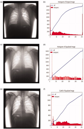
Figure 2. Flowchart of the proposed method. (a) Segmentation of Original Image. (b) Segmentation of GHE Image. (c) Segmenatation of CLAHE Image.

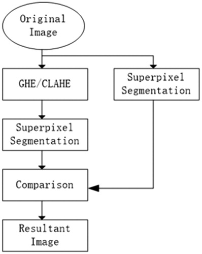
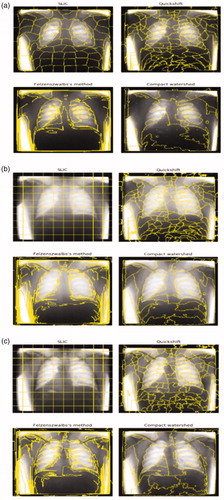
Figure 3. Comparison of segmentation results using four superpixel segmentation algorithms (a) superpixels of the original image (b) shows the superpixels generated for GHE image and (c) shows the superpixel segments of CLAHE image. (a) Input image (b)superpixel segmentation (c) GHE (d) CLAHE.

2. Histogram equalization (HE)

It is one of the most celebrated techniques of image enhancement since it is simple and produces visually pleasing results out of noisy or dark images. Basic histogram equalization is called Global Histogram Equalization (GHE) because it does enhancement globally. It is known with different names such as Classical HE [13], Traditional HE [14], Conventional HE and Typical HE [15]. Suppose that X = {X(i,j)} is a given image, which consists of L number of discrete gray levels. {X₀, X₁, …, X_L−1} represents the intensity of the image at some spatial location (i,j), assuming that X(i,j) ∈ {X₀, X₁, …, X_L−1}.

A discrete function is the histogram of digital image and can be written as: (1) $$\mathit{h}\left({\mathit{X}}_{\mathit{k}}\right) ={\mathit{n}}_{\mathit{k}}, \mathit{f} \text{or} \mathit{k}= 0,1, \dots , \mathit{L}-1$$(1) where X_k is the k-th gray level and n_k denotes the number of times that gray level (X_k) appears in the image. Moreover, as discussed by Wang and Ye [16] in statistical terms it is the probability distribution of each gray level. The Probability Density Function (PDF) for a given image X and intensity X_k, p(X_k) , is given by: (2) $$p\left(X_k\right)=\frac{n_k}{N}, f or k=0,1, \dots , L-1$$(2)

Whereas, N equals the total number of samples or pixels and n_k is the number of times k-th gray level appears in the image. If we compare Equations (1)(1) $$\mathit{h}\left({\mathit{X}}_{\mathit{k}}\right) ={\mathit{n}}_{\mathit{k}}, \mathit{f} \text{or} \mathit{k}= 0,1, \dots , \mathit{L}-1$$(1) and (2(2) $$p\left(X_k\right)=\frac{n_k}{N}, f or k=0,1, \dots , L-1$$(2) ) then it is clear that PDF is a normalized histogram. It simply maps the intensities of input images in such a way that the intensities of output images are spread over the full range of intensities. In order to achieve this, the Cumulative Distribution Function (CDF) of the input image is used as the mapping function. A normalized histogram can be identified as the probability density function of the random signal. So according to the Probability Distribution Function (PDF) Equation (2)(2) $$p\left(X_k\right)=\frac{n_k}{N}, f or k=0,1, \dots , L-1$$(2) , the Cumulative Distribution Function (CDF) for an intensity X_k, c (X_k) is defined as: (3) $$c\mathrm{ }\left(X_k\right)=f\mathrm{ }or\mathrm{ }k=\mathrm{0,1},\mathrm{ }\dots ,\mathrm{ }L-1\mathrm{ }$$(3)

2.1. Adaptive histogram equalization

Global histogram equalization does not work effectively for images that contain local regions of low contrast and bright or dark regions. In this case, local histogram equalization LHE comes into action. It works by taking into account only small regions and based on their local CDFs, performs contrast enhancement of those regions. Examples of LHE method include Adaptive Histogram Equalization (AHE) [17,18], Contrast Limited Adaptive HE (CLAHE) [17], Interpolated Adaptive HE (IAHE), Weighted Adaptive HE (WAHE) [17], Non-Overlapped Block HE (NOBHE) [19], Partially Overlapped Sub-Block HE (POSHE) [20], Cascaded Multistep Binomial Filtering HE (CMBFHE) [21], Fast Local Histogram Specification (FLHS) [22] and Conditional Sub-Block Bi-HE (CSBHE) [23]. Pizer et al. have defined the AHE using a tiled window with interpolated mapping in their paper. This method enhances the global contrast but at the cost of enhancing the noise in regions with small intensity range.

2.2. Contrast limited adaptive histogram equalization (CLAHE)

In order to overcome the noise enhancement artifact of AHE, this method takes one extra step to clip the histogram before computing the CDF as a mapping function. It also introduces an additional parameter that defines the level where to clip the histogram. As explained by the Pizer et al. [17,18], contrast enhancement is also known as the slope of the function mapping input intensities to the output intensities. If we limit the height of the histogram to a specific level, we can infer that we can also limit slope of the CDF mapping function as well as the level of contrast enhancement. Thus, the mapping function m(i) is proportional to the cumulative histogram. (4) $$m\left(i\right)=\left(\mathit{\text{Display Range}}\right)\mathrm{\hspace{0.17em}*\hspace{0.17em}}\left(\frac{\mathit{\text{Cumulative Histogram\hspace{0.17em}}}\left(i\right)}{\mathit{\text{Region Size}}}\right)$$(4)

We will make use of global histogram equalization GHE and CLAHE to equalize the histogram of input image first and then we will perform the superpixel segmentation using four techniques that are discussed in section 4. Figure 1 shows the original image (a), its global histogram equalized image (c) and the contrast limited adaptive histogram equalized image (e). The histogram of each image is also shown in Figure 1(b), (d) and (f) respectively.

3. Superpixel segmentation

Superpixels are gaining popularity in the various computing applications because of their perceptual meaningfulness and computational efficiency. They significantly decrease the complexity of certain image processing tasks. Variety of features is available for grouping pixels into superpixels, such as brightness, intensity, texture, contour and good continuation. Superpixels are used in several fields such as image segmentation [24], skeletonization [25], object localization [26], recognition, image indexing and body model estimation [27]. Each superpixel in an image is a consistent unit of similar pixels, such as, similar in color or texture. They are the result of over-segmentation. Broadly speaking, Achanta et. al. [28] categorized them into two classes, gradient-ascent based and graph-based algorithms. Graph-based algorithm treats each pixel as a node in a graph, and edge weights between two nodes are set proportional to the similarity between pixels, Felzenszwalb’s algorithm is an example of graph-based algorithms. However, gradient-ascent based algorithms start by operating over an initial rough clustering. It is an iterative process where during each iteration new clusters are refined from the previous iteration to obtain better segmentation until convergence is achieved. SLIC, Quick shift, and Watersheds are of this class. These algorithms behave differently when an original image and histogram equalized image is subjected to them, we will make use of all of these four algorithms. In this section, we will briefly look into these segmentation algorithms. Since we are not primarily concerned with the number of superpixels, we will not explicitly control the number of superpixels.

3.1. Felzenszwalb’s algorithm

This efficient and fast image segmentation algorithm proposed by Felzenszwalb, P.F. and Huttenlocher is prevalent in the computer vision field. It has only one scaling factor that affects the size of a segment. The number and actual size of segments may vary significantly, depending on the local contrast of images. However, it does not provide explicit control over the number of segments. This algorithm provides segmentation of both real and synthetic images and widely known as a segmentation algorithm rather than a superpixel algorithm. We will see that it works normally with original as well as histogram equalized images. In general, the input to the graph based algorithms is a graph G = (V, E), with n vertices and m edges [29]. The output is a segmentation of V into S = (C₁,C₂, …, C_r) components. Dijkstra’s algorithm is used for computing the shortest paths in the undirected graph defined on these grid positions. It has a complexity of O(NlogN).

3.2. Quick shift algorithm

It is a mode seeking two dimensional (2D) algorithm used for image segmentation. The algorithm relies on the approximation of kernelized mean-shift. It makes use of the Parzen density estimation. Let us consider N number of data points denoted as $x_1,x_2,\dots ,x_N\in X=R^d$, then a mode-seeking algorithm like quick shift begins by computing the Parzen density estimate: (5) $${P\left(x\right)=\frac{1}{N}\sum _{i=1}^{N}k(x-x}_i),x\in R^d$$(5)

Similar to the SLIC algorithm, quick shift is also applied to the 5 D space, which not only consists of image location but also color information. However, contrary to SLIC, it cannot control the number or size of superpixels explicitly. One of the advantages of quick shift algorithm is that it simultaneously computes ordered segmentation on multiple scales.

3.3. Watersheds algorithm

It makes intelligent use of the watershed transformation and topological gradient approach. Instead of taking a color image as input, it takes a grayscale gradient image, where bright pixels represent boundaries among segments or regions. It obtains watersheds or lines that separate catchment basins [30]. It takes gray level images as topographic reliefs and each of the reliefs is flooded from its minima. A dam is built when two lakes merge, the set of all dams define the so-called watershed. This representation of watersheds simulates the natural flooding process [31]. It takes the input image as a landscape, where bright pixels form high peaks. Each individual basin ultimately makes a unique segment. Just like SLIC. It is also a single parameter algorithm but there is another compactness parameter that makes it tougher for markers to flood faraway pixels. This results in the uniform and compact watershed regions or segments.

3.4. SLIC superpixels

The SLIC uses k-means clustering for superpixel generation, which makes it relatively easy and fast. In addition, by default, k is the lone parameter for setting the required number of superpixels. Hence, we can control the size indirectly by choosing the appropriate number of superpixels. SLIC works for both color and grayscale images, and this provided us the opportunity to use SLIC on grayscale images before and after histogram equalization to test their original and histogram equalized nature. Most of the superpixel generation methods do not provide explicit control over the compactness and even the number of superpixels which we wish to generate. Nevertheless, in SLIC we have firm control over the number, size as well as the compactness of the superpixels. In this paper, we make use of the compactness parameter to show that superpixels generated for a given image before and after histogram equalization are different for the same compactness parameter setting. We have used the proposed method on various medical images. Moreover, as discussed in section 5, we also show that other superpixel segmentation methods work normally without differentiating between original and histogram equalized image. SLIC algorithm [32] is divided into three main steps. First is the initialization step in which clusters are initialized; in the second assignment step each pixel is associated with the nearest cluster center if search region overlaps its location. Finally, in the third step cluster centers are updated to become the mean vector of all the pixels belonging to the cluster. Nevertheless, the literature shows that by selecting small values of the compactness parameter spatially more compact (square shaped) superpixels could be obtained. In our method, we select the value of compactness parameter to be the same for image segmentation before and after equalization. Whereas the number of superpixels k can be selected arbitrarily. The resulting superpixels of histogram equalized images will be the same as corresponding superpixels in the original image.

4. Proposed technique

In this section, we present the basic steps used for analyzing histogram equalized images(as Figure 2 shown), these steps includes: histogram equalization, superpixel segmentation and analyzing the histogram equalized images.

The flowchart in Figure 2. illustrates the steps used in our method. The original grayscale image is inputted to both the superpixel segmentation (SLIC, quick shift, watersheds, and Felzenszwalb) and histogram equalization (GHE and CLAHE) algorithms for relevant segmentation and equalization respectively. In the next step, only histogram equalized images are again inputted to all four superpixel segmentation algorithms and resultant images are acquired for comparison.

At this point, we have four superpixelized images in Figure 3(a), and four global histogram images with superpixels in Figure 3(b) and four CLAHE images with superpixels as shown in Figure 3(c). In the final stage, a comparison is done among original image, global histogram equalized GHE images and adaptive histogram equalized CLAHE images with superpixel segments. The resultant image is the histogram equalized image with compact SLIC superpixels.

5. Comparison

In this section, we compare superpixels generated by four publicly available algorithms, namely, SLIC, Quick shift, Watersheds and Felzenszwalb. In general, superpixels are used at a pre-processing stage in vision applications. In this paper, we have used superpixels at post-processing stage. Firstly, the output images obtained from two histogram equalization processes i.e. GHE and CLAHE are segmented into superpixels by using four segmentation algorithms. Figure 3(a) at top-right is the result of SLIC, at top-left is the result of the quick shift, at bottom-left is the result of Felzenszwalb and figure at bottom-right shows the superpixels generated by the watersheds algorithm for the original image. Figure 3(b) is the result of superpixel segmentations for globally histogram equalized image and Figure 3(c) shows the superpixel segmentations for CLAHE image. As one can clearly see that only SLIC superpixels (Figure 3(b) top left) are compact and uniform if the given image is histogram equalized as compared to the Figure 3(a) top left image which is SLIC superpixel segmentation before histogram equalization. It should be noted here that the shape of superpixels clearly varies even for the same parameter settings of SLIC. The resulting SLIC superpixels in Figure 3(b) and (c) are spatially more compact but spectrally they are more heterogeneous. Pixels belonging to the same superpixel are of similar nature, it also simplifies their nature as compared to individual pixels, which we had before histogram equalization. Yellow colored lines superimposed on the segmented images are called the superpixel boundaries and they separate one superpixel or segment from the other. They are shown here in the output image as we are not interested in the result of image enhancement or histogram equalization but we want to know the nature of images based on superpixels. Without these boundaries, image will look similar to the image obtained after histogram equalization process. Experiments show that SLIC superpixels for original low contrast images are of arbitrary shape. However, for histogram equalized images it produces compact and uniform superpixels.

Moreover, other three algorithms work normally on both original and histogram equalized images as shown in Figure 3. Thus, SLIC superpixels clearly distinguish between an original image and its histogram equalized version. The comparison is done to show the robustness of the SLIC superpixels and our technique. A Quantitative comparison is also shown in Table 1.

Table 1. Comparison of superpixels.

Before HE	SLIC	Quick shift	Felzenszwalb	Watershed
No. of Superpixels	100	163	195	100
Compactness	Non-uniform	Non-uniform	Non-uniform	Non-uniform
Parameters	1	2	1	2
After GHE	SLIC	Quick shift	Felzenszwalb	Watershed
No. of Superpixels	100	186	219	100
Compactness	Uniform	Non-uniform	Non-uniform	Non-uniform
Parameters	1	2	1	2
After CLAHE	SLIC	Quick shift	Felzenszwalb	Watershed
No. of Superpixels	100	190	266	100
Compactness	Uniform	Non-uniform	Non-uniform	Non-uniform
Parameters	1	2	1	2

5.1. Additional test images

With the following experiments, by using different images we want to show the performance and efficiency of the proposed method. Figure 4. shows some of the medical test images and generated results. Original images are placed in column (a), segmentation of original images is in column (b) and column (c) shows the segmentation of global histogram (GHE) images and column (d) shows the segmentation of CLAHE images. Our proposed method analyses different test images and gives satisfactory results to distinguish between original and histogram equalized image. Further, in order to show the robustness of proposed method, we have tested some additional publicly available medical image databases of different types as mentioned in Table 2.

Figure 4. Some test images: An input image (column (a)), its superpixel segmentation by using four segmentation algorithms (b). Our work is focused on generating superpixel segments of GHE image (c), of CLAHE image (d) and compare their results.

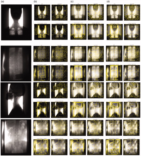
Table 2. Some publicly available datasets used for performance evaluation of the proposed method.

Name of dataset	Download link
BrainWeb	http://brainweb.bic.mni.mcgill.ca
Harvard medical school website	http://www.med.harvard.edu
Open Access Biomedical ImageSearch Engine	https://openi.nlm.nih.gov

6. Conclusion

Histogram equalized images are not always bright and visually different from the original images. Making it is hard to recognize a histogram equalized image. We present a novel technique for the testing and validity of histogram equalized medical images using SLIC. We have observed that SLIC superpixels are biased towards the histogram equalized images. We have also performed a comparison of SLIC with other popular methods of segmentation. This research will assist in image enhancement process for differentiating between enhanced/histogram equalized and original images. Looking toward the future, we would like to analyze the color images with a different intensity or contrast level for histogram matching.

Disclosure statement

No potential conflict of interest was reported by the authors.

Additional information

Funding

This work is supported by Industrial Prospective Project of Jiangsu Technology Department under Grant No. BE2017081.

References

- Celik T, Tjahjadi T. Automatic image equalization and contrast enhancement using gaussian mixture modeling. IEEE Trans Image Process. 2012;21:145.
- Lee E, Kim S, Kang W, et al. Contrast enhancement using dominant brightness level analysis and adaptive intensity transformation for remote sensing images. IEEE Geosci Remote Sensing Lett. 2013;10:62–66.
- Huang SC, Cheng FC, Chiu YS. Efficient contrast enhancement using adaptive gamma correction with weighting distribution. IEEE Trans Image Process. 2013;22:1032–1041.
- Zanaty EA, Afifi A. A watershed approach for improving medical image segmentation. Comp Methods Biomech Biomed Eng. 2013;16:1262–1272.
- Patil DV, Mulla A, Chougale SB. Medical Image Enhancement Using GMM: A Histogram approach. Paper presented at: International Journal of Scientific and Research Publications (IJSRP), 2015(5), Issue 12.
- Chen X, Zhang F, Zhang R. Medical image segmentation based on SLIC superpixels model[J]. Proceedings of the SPIE. 2017;245:1024502.
- Criminisi A. Machine learning for medical images analysis. Med Image Anal. 2016;33:91–93.
- Baxter J, Gibson E, Eagleson R, et al. The semiotics of medical image segmentation. Med Image Anal. 2018;44:54–71.
- Bruijne MD. Machine learning approaches in medical image analysis: from detection to diagnosis. Med Image Anal. 2016;33:94–97.
- Goceri E, Goceri N. Deep Learning in Medical Image Analysis: Recent Advences and Future Trends. Paper Present at: International Conferences Computer Graphics, Visualization, Computer Vision and Image Processing. 2017. Lisbon, Portugal, 305–310.
- Dora L, Agrawal S, Panda R, et al. State of the art methods for brain tissue segmentation: a review. IEEE Rev Biomed Eng. 2017;99:1–91.
- Smistad E, Falch TL, Bozorgi M, et al. Medical image segmentation on GPUs-a comprehensive review. Med Image Anal. 2015;20:1–18.
- Menotti D, Najman L, Facon J, et al. Multi-histogram equalization methods for contrast enhancement and brightness preserving. IEEE Trans Consumer Electron. 2007;53:1186–1194.
- Wang Q, Ward RK. Fast image/video contrast enhancement based on weighted thresholded histogram equalization. IEEE Trans Consumer Electron. 2007;53:757–764.
- Chen SD, Ramli AR. Contrast enhancement using recursive mean-separate histogram equalization for scalable brightness preservation. IEEE Trans Consumer Electron. 2003;49:1301–1309.
- Wang C, Ye Z. Brightness preserving histogram equalization with maximum entropy: a variational perspective. IEEE Trans Consumer Electron. 2005;51:1326–1334.
- Pizer SM, Amburn EP, Austin JD, et al. Adaptive histogram equalization and its variations. Comp Vision Graphics Image Proc. 1987;39:355–368.
- Kong N. A literature review on histogram equalization and its variations for digital image enhancement. Int J Innovation Management Technol. 2013;386–389.
- Gonzalez RC, Woods RE. Digital image processing. 2nd ed. Boston, MA, USA: Prentice-Hall of India; 2002.
- Kim JY, Kim LS, Hwang SH. An advanced contrast enhancement using partially overlapped sub-block histogram equalization. IEEE Trans Circ Sys Video Technol. 2001;11:475–484.
- Lamberti F, Montrucchio B, Sanna A. CMBFHE: a novel contrast enhancement technique based on cascaded multistep binomial filtering histogram equalization. IEEE Trans Consumer Electron. 2006;52:966–974.
- Liu HD, Yang M, Gao Y, et al. Fast local histogram specification. IEEE Trans Circuits Syst Video Technol. 2014;24:1833–1843.
- Saffarian N, Zou JJ. DNA microarray image enhancement using conditional sub-block bi-histogram equalization. Paper presented at: IEEE International Conference on Video & Signal Based Surveillance. IEEE Computer Soc. 2006;86.
- Belaid LJ, Mourou W. Image segmention: a watershed transformation algorithm. Image Anal Stereol. 2011;28:93–102.
- Levinshtein A, Dickinson S, Sminchisescu C. Multiscale symmetric part detection and grouping. Paper presented at: International Conference on Computer Vision. IEEE 2010;104:2162–2169.
- Fulkerson B, Vedaldi A, Soatto S. Class segmentation and object localization with superpixel neighborhoods. Paper presented at: International Conference on Computer Vision. IEEE, 2009:670–677.
- Mori G. Guiding model search using segmentation. Paper presented at: International Conference on Computer Vision. IEEE 2005;1417–1423.
- Achanta R, Shaji A, Smith K, et al. SLIC superpixels compared to state-of-the-art superpixel methods. IEEE Trans Pattern Anal Mach Intell. 2012;34:2274–2282.
- Felzenszwalb PF, Huttenlocher DP. Efficient graph-based image segmentation. Int J Comput Vis. 2004;59:167–181.
- Vincent L, Soille P. Watersheds in digital spaces: an efficient algorithm based on immersion simulations. IEEE Trans Pattern Anal Machine Intell. 1991;13:583–598.
- Körbes A, Vitor GB, Ferreira JV, et al. A Proposal for a Parallel Watershed Transform Algorithm for Real-Time Segmentation. Paper presented at: WVC’2009.
- Ren X, Malik J. Learning a classification model for segmentation. Paper presented at: International Conference on Computer Vision. IEEE 2003;10–17.