Deep learning for assessing liver fibrosis based on acoustic nonlinearity maps: an in vivo study of rabbits

Abstract

This study aimed to assess liver fibrosis in rabbits by deep learning models based on acoustic nonlinearity maps. Injection of carbon tetrachloride was used to induce liver fibrosis. Acoustic nonlinearity maps, which were built by data of echo signals, were used as input data for deep learning model. Convolutional neural network (CNN), CNN combined with support vector machine (SVM), CNN combined with random forest and CNN combined with logistic regression were used as deep learning model. Nested 10-fold cross-validation was used to search hyperparameters and evaluate performance of models. Histologic examination of liver specimens of the rabbits was performed to evaluate the fibrosis stage. Receiver operator characteristic curve and area under curve (AUC) were used for estimating the probability of the correct prediction of liver fibrosis stages. A total of 600 acoustic nonlinearity maps were used. Model of CNN combined with SVM demonstrated the best diagnostic performance compared with all other methods for diagnosis of significant fibrosis (≥F2, AUC = 0.82), advanced fibrosis (≥F3, AUC = 0.88) and cirrhosis (F4, AUC = 0.90). Model of CNN showed the second highest AUCs. The deep learning model based on acoustic nonlinearity maps demonstrated potential for evaluation of liver fibrosis.

Keywords:

• Deep learning
• liver fibrosis
• acoustic nonlinearity
• ultrasound

Introduction

Liver fibrosis, which may be caused by hepatic injury such as virus infection and alcohol abuse, is a stage progressing to cirrhosis [1]. Patients with cirrhosis might suffer from several complications, such as hepatocellular carcinomas, esophageal varices and/or hepatic failure [2]. Staging fibrosis stages is essential for prognosis, surveillance and management of patients with liver fibrosis [3,4]. The golden standard of assessing fibrosis stages is liver biopsy [5,6]. However, liver biopsy is invasive so that it may lead to various potential complications such as bleeding and rupture. Meanwhile, sampling errors also limit the diagnostic accuracy. Biomarkers show suboptimal diagnostic accuracy compared with imaging methods [7,8]. Conventional ultrasound, CT and MRI are not sensitive enough for predicting fibrosis. Ultrasound-based elastography is studied for staging liver fibrosis in recent years with good performance [9,10]. Shear wave speed is measured in ultrasound-based elastography such as Transient Elastography and Shear Wave Elastography. Diagnostic accuracy is high for the detection of significant and advanced fibrosis and cirrhosis (area under curve (AUC) > 0.90) [9]. Nevertheless, the cutoff values among various kinds of elastography machines require further investigation. Breath could also affect the reliability and accuracy [11].

In recent years, acoustic nonlinearity has been studied for tissue characterizing imaging [12,13]. Conventional ultrasound theory used in B-mode ultrasound hypothesizes that sound wave propagates linearly in the medium. However, in fact, sound wave can be distorted in the propagation and generate harmonic wave [14]. The phenomenon of wave distortion and harmonic generation is called acoustic nonlinearity in medium. Nonlinear parameter B/A is an indicator to assess the effect of nonlinearity [15]. The differences of nonlinear parameter B/A can be detected even in the medium that has similar linear acoustic parameter (for example acoustic impedance and sound of speed) [15]. Hence, nonlinear parameter B/A is considered to be more sensitive to pathological feature than linear acoustic parameter. In last two decades, several nonlinear imaging methods have been proposed to estimate acoustic nonlinearity. Transmission methods that required supersensitive acoustic hydrophones and reflection methods that needed metal reflector are 2 methods to calculate acoustic nonlinear parameter B/A precisely [16,17]. Both two methods are not appropriate for the study in vivo. Methods using echo signals to calculate acoustic nonlinear parameter without reflector were able to be applied on study in vivo [13,15,18]. However, the precision was suboptimal compared with transmission methods.

It has been identified that nonlinearity parameter B/A varies between normal liver and fibrotic liver [17]. However, the supersensitive acoustic hydrophones or reflective plates are required to precisely calculate nonlinearity parameter B/A and these devices limit the measurement of nonlinearity parameter B/A in vivo [12,15]. To estimate the nonlinearity of liver fibrosis in vivo, methods using echo signals are required. Several studies verified that the ratio of amplitude of a high voltage transmit to amplitude of a low voltage transmit could be used to show the level of the acoustic nonlinearity. Fatemi et al. presented a method to display the acoustic nonlinearity basing on the ratio of amplitude of high density transmit to amplitude of low density transmit [19]. Chen et al. also introduced a similar approach to image the acoustic nonlinearity through the ratio of echo amplitude of different power levels [15]. Nevertheless, we do not find related researches using echo signals without reflective plates to assess nonlinearity of liver fibrosis.

Machine learning is one of the prime branches of artificial intelligence, which has the ability to learn and improve from experience [20]. Deep learning technique, as one of machine learning technique, has attracted significant attention in machine learning field and obtained spectacular achievement, such as computer assisted diagnosis for tumor. Convolutional neural networks (CNN) is a widely investigated model of deep learning, which has been proven efficient in medical imaging recognition, especially in the fields of differential diagnosis between benign and malignant tumor and stroke [20–22]. Prediction of liver fibrosis stages is also a field in which CNN had been applied recent years. CNN using conventional B-mode ultrasound images and elastography images as input data displayed good diagnostic performance for liver fibrosis [23]. Hidden layers embedded in CNN automatically extract features that may not be detectable in humans’ naked eyes [24]. However, to our knowledge, there is no study applying CNN methods on acoustic nonlinearity information for diagnosis liver fibrosis. We hypothesize that CNN can extract useful nonlinear information embedded in echo signals to diagnose liver fibrosis instead of computing exact nonlinearity parameter B/A. Then, liver fibrotic stages can be classified by CNN.

In this study, we proposed to establish models of liver fibrosis in New Zealand rabbits. Then, acoustic nonlinearity maps were built through echo signals. CNN and machine learning methods were used to set up classification models. The diagnostic performance of classification models for liver fibrosis were assessed.

A brief introduction to the classification models are as follows. In this study, CNN, CNN combined with support vector machine (SVM), CNN combined with random forest and CNN combined with logistic regression will be used as classification model.

CNN is a deep feed-forward neural network model for processing data with mesh-like features. The sparse connection with the parameter weight sharing methods is integrated by CNN, which results in a significant reduction in the number of training parameters and effective avoidance of algorithm over-fitting. Meanwhile, the back-propagation algorithm is used to update the model parameters. A typical CNN structure consists of feature extraction network and classification network. Convolutional layers and pooling layers are the main components in feature extraction network. Convolutional layer contains a bunch of learnable filters (kernels) to convolve input data to generate feature maps as the input to the next layer. Once the linear transformations are completed, non-linear activation functions are applied to the output of filters. Behind the convolutional layer is the pooling layer. In pooling layer, the dimension and quantity of trainable parameters are diminished by pooling kernels. The process of pooling is aimed to control over-fitting and increase robustness to minor variations in the input data. In classification network, fully connected layer applies a linear transformation to extract and connect features. The softmax classifier is located behind fully connected layers to ensure that the output vector is normalized to sum to 1, reflecting an estimate of the posterior class distribution [25].

In model of CNN combined with machine classifiers, the classification network is replaced by the classifier, including SVM, random forest and logistic regression. The goal of SVM is to locate the super hyperplane in the feature space with the biggest margin between positive and negative samples. As a result, an SVM classifier can acquire strong generalization ability from test examples during the testing phase. It has a number of distinct benefits when it comes to addressing small sample, multi-class, nonlinear, and high-dimensional problems. Random forest is a supervised machine learning method that constructs numerous decision trees to generate a more precise prediction or classification: the algorithm's output matches the majority of the trees' output. It can weaken the overfitting problem compared with decision trees. Logistic regression is a generalized linear model that uses a logistic function to model a binary dependent variable. Linear regression analyzes binary outcomes and assumes that the relationship between the outcome and independent variables follows a line, which can be used in computer aided diagnosis and data mining.

Materials and method

Animal models

The use of experimental animals was approved by the Animal Ethics Committee of the West China Hospital, Sichuan University. All experiments were complied with the protocols and guidelines of the humane treatment of animals for research and teaching. All experiments were complied with the protocols and guidelines of the humane treatment of animals for research and teaching. A total of 80 rabbits (mean age ± SD = 124.5 ± 19 days, weighed about 2.5 kg) were enrolled at the beginning of the study. These 80 rabbits were randomly divided into experimental group (n = 70) and control group (n = 10). For the rabbits in control group, olive oil was subcutaneously injected once a week with a dose of 0.3 ml/kg body weight twice a week. For the rabbits in experimental group, carbon tetrachloride (CCl₄) in olive oil with a concentration of 40% was injected subcutaneously with a dose of 0.3 ml/kg body weight to induce liver fibrosis, twice a week. Starting from the fourth week, 4 rabbits from experimental group and 1 rabbit from control group were randomly selected to be examined by ultrasound every week. Then, the selected rabbits were sacrificed for histological examination.

Acquisition of echo signals

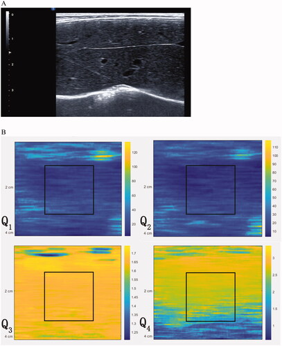
iMago C21 ultrasound system (Saset Healthcare Inc., Chengdu, China) equipped with a linear transducer (frequency ranging from 5 to 10 mHz) was used for acquisition of echo signals. Hair of upper abdomen was removed to reduce the attenuation of ultrasound wave. The rabbits were anesthetized by intramuscular administration of 0.2 ml/kg zolazepam/tiletamine and 2 mg/kg xylazine hydrochloride. Transducer was positioned at subxiphoid or subcostal. Frequency, depth, focus depth and pulse cycle were set as 5 mHz, 4 cm, 2 cm and 5 cycles, respectively. Pulses with two different excitation voltages were transmitted. Lower excitation voltage was 39v and higher excitation voltage was 69v. While the liver was displayed clearly, echo signals of the whole image were recorded (Figure 1(A)). Ten times of echo signals were acquired for each rabbit.

Figure 1. (A) B-mode ultrasound images while recording echo signals. (B) Acoustic nonlinearity map was composed of 4 channels derived from 4 imaging functions (Q₁, Q₂, Q₃ and Q₄) with a total of 740 * 110 * 4 pixels. The region of interest (ROI) with size of 2 cm * 2 cm was positioned 1 cm below the liver capsule in each acoustic nonlinearity map.

Histological evaluation

Once the echo signal data was recorded completely, the rabbit was sacrificed. Liver specimens with size of 1 cm³ were fixed in 10% formalin and stained with hematoxylin and eosin (H&E) and Masson’s trichrome. METAVIR scoring system (modified according to the histopathological characters of CCl₄- induced liver lesion) was used for evaluation of liver fibrosis [26]. F0(without fibrosis), F1(fibrosis without septa), F2(fibrosis with few septa), F3(fibrosis with numerous septa but without pseudo-lobule) and F4(cirrhosis) were used to detail the stages of fibrosis. The stages of ≥ F2, ≥F3 and F4 indicated the significant fibrosis, advanced fibrosis and cirrhosis, respectively. Pathological assessment was performed by an experienced pathologist, who was blinded to the animal data and the ultrasonic graphics.

Acoustic nonlinearity map

Acoustic nonlinearity maps were used as the input data of CNN.

Acoustic nonlinear propagation can be demonstrated by KZK equation and Westervelt equation [27]. T.jotta and Tjotta proposed a nonlinear differential equation to discuss the relationship between KZK and Westervelt equation [28]. For density$\mathrm{ }\rho (x, y, z, t):$ (1) $$\left({\nabla }^2-\frac{1}{c^2}\frac{{\partial }^2}{\partial t^2}\right)\rho =\frac{\eta }{c_0^4}\frac{{\partial }^3\rho }{\partial t^3}-\frac{\beta }{{\rho }_0{c}_0^2}\frac{{\partial }^2}{\partial t^2}{\left(\rho -{\rho }_0\right)}^2,$$(1) where ${\mathrm{c}}_0,\mathrm{ }{\rho }_0$ and $\mathrm{\eta }$ are velocity, density and viscosity, respectively. $\mathrm{\beta }=(1+B/2A)$ denotes nonlinear parameter. Nikoonahad and Liu have developed an approximate solution of this equation under narrow-band condition [18]. Given a source located at the origin in a cylindrical coordinate system$\mathrm{ }(r, z),$ a paraxial approximation of the solution in the Gaussian form was given: (2) $$\left|{\rho }_1\left(r,z\right)\right|=H_1{e}^{-{\alpha }_{1}z}{c}_{1}s\mathit{ech}\left(e^{-{2\alpha }_{1}z}{c}_1\frac{\beta k_1}{2{\rho }_0}ln\frac{z}{z_0}\right),$$(2) (3) $$\left|{\rho }_2\left(r,z\right)\right|=H_2{e}^{-{\alpha }_2\mathrm{z}}{c}_{1}t\mathit{anh}\left(e^{-{2\alpha }_{1}z}{c}_1\frac{\beta k_1}{2{\rho }_0}ln\frac{z}{z_0}\right),$$(3) where ${\rho }_1$ and ${\rho }_2$ represent the density variation with spatial distribution in fundamental frequency and second harmonic frequency, $H$ denotes the diffraction term [18], ${\alpha }_1={{\omega }_1}^2\eta /2{c_0}^2$ and $k_1$ are attenuation coefficient and wave number at frequency ${\omega }_1,$ $c_1$ denotes amplitude of the fundamental frequency component at $z_0.$ The sech(.) term represents the depletion of the fundamental and the tanh(.) term predicts the growth of the second harmonic.

For clinical ultrasonic array probes, the amplitudes of the received signal can be computed by the sound field integrated over the transducer aperture [18], in the following form: (4) $$V_{\mathit{out}}\left({\omega }_1\right)=K{V}_{in}\sec h\left(e^{-{2\alpha }_{1}z}C{V}_{in}\frac{\beta k_1}{2{\rho }_0}ln\frac{z}{z_0}\right),$$(4) (5) $$V_{\mathit{out}}\left({\omega }_2\right)=K{V}_{in}\mathit{tan}h\left(e^{-{2\alpha }_{1}z}C{V}_{in}\frac{\beta k_1}{2{\rho }_0}ln\frac{z}{z_0}\right),$$(5) where $V_{\mathit{out}}$ denotes envelope of the received signal which is derived from radio frequency signals via quadrature demodulation, $V_{in}$ is input voltage amplitude, ${\omega }_1$ and ${\omega }_2$ represent fundamental frequency and second harmonic frequency, $K$ denotes the diffraction effects and the system gain [18,19], $C$ denotes a constant representing the efficiency of transducer, $z$ is the depth.

To acquire the nonlinearity information in received signals, we would use two-pulse transmission with different peak-to-peak exciting voltages to build the maps. According to the nonlinear theory of ultrasound propagation model, the nonlinearity may be estimated by the ratio of the fundamental amplitude to the second harmonic amplitude or the ratio of a high voltage transmit to a low voltage transmit [15,18]. For fundamental component of echo signal, imaging function $Q_1$ is defined as the ratios of the fundamental amplitude to the second harmonic amplitude with low excitation voltage: (6) $$Q_1=\frac{V_{\mathit{out}1}\left({\omega }_1\right)}{V_{\mathit{out}1}\left({\omega }_2\right)}=\frac{\mathrm{ }K{V}_{in1}\mathit{s}\mathit{ec}h\left(e^{-{2\alpha }_{1}z}C{V}_{in1}\frac{\beta k_1}{2{\rho }_0}ln\frac{z}{z_0}\right)}{K{V}_{in1}\mathit{t}\mathit{an}h\left(e^{-{2\alpha }_{1}z}C{V}_{in1}\frac{\beta k_1}{2{\rho }_0}ln\frac{z}{z_0}\right)}=\frac{\mathit{s}\mathit{ec}h\left(T\beta V_{in1}\right)}{\mathit{t}\mathit{an}h\left(T\beta V_{in1}\right)}=\frac{1}{\mathit{s}\mathit{in}h\left(T\beta V_{in1}\right)\mathrm{ }},$$(6) where $V_{\mathit{out}1}\left({\omega }_1\right)\text{ and }{V}_{\mathit{out}1}\left({\omega }_2\right)$ denote envelopes of the fundamental and second harmonic echo signal under condition of low excitation pulse voltage, $V_{in1}$ is the low excitation pulse voltage, $T=e^{-{\alpha }_{1}z}C\frac{k_1}{2{\rho }_0}\mathrm{l}\mathrm{n}\frac{z}{z_0},$ which is related to probe transfer efficiency, depth and medium density [15].

In a same way, we defined imaging function $Q_2$ as the ratio of the fundamental amplitude to the second harmonic amplitude with high excitation voltage: (7) $$Q_2=\frac{V_{\mathit{out}2}\left({\omega }_1\right)}{V_{\mathit{out}2}\left({\omega }_2\right)}=\frac{1}{\text{sin}h\left(T\beta V_{in2}\right)},$$(7) where ${\mathrm{V}}_{\mathit{out}2}\left({\omega }_1\right)\text{ and }{V}_{\mathit{out}2}\left({\omega }_2\right)$ denote envelopes of the fundamental and second harmonic echo signal under condition of high excitation pulse voltage, $V_{in2}$ is the high excitation pulse voltage.

Imaging function $Q_3$ were defined as the ratio of the fundamental amplitude using two different excitation voltages for $V_{in1}$ and $V_{in2}$ gives: (8) $$Q_3=\frac{V_{\mathit{out}1}\left({\omega }_1\right)}{V_{\mathit{out}2}\left({\omega }_1\right)}=\frac{V_{in1}}{V_{in2}}\mathrm{*}\text{sec}h\left(T\beta V_{in1}\right)\mathrm{*}\text{cos}h\left(T\beta V_{in2}\right).$$(8)

Similarly, we defined $Q_4$ as ratio of the second harmonic amplitude using two different excitation voltages for $V_{in1}$ and $V_{in2}:$ (9) $$Q_4=\frac{V_{\mathit{out}1}\left({\omega }_2\right)}{V_{\mathit{out}2}\left({\omega }_2\right)}=\frac{V_{in1}}{V_{in2}}\mathrm{*}\text{tan}h\left(T\beta V_{in1}\right)\mathrm{*}\text{cot}h\left(T\beta V_{in2}\right)$$(9)

Imaging functions $Q_1-Q_4$ represent the level of additional nonlinear attenuation of echo signals due to the nonlinear effects.

We used the four imaging functions $Q_1,\mathrm{ }{Q}_2,\mathrm{ }{Q}_3$ and $Q_4$ as 4 channels to compose the acoustic nonlinearity map with a total of 740 * 110 * 4 pixels (Figure 1(B)). One region of interest (ROI) with size of 2 cm * 2 cm was positioned 1 cm below the liver capsule in each acoustic nonlinearity map.

Classification model

CNN, CNN combined with support vector machine (SVM), CNN combined with random forest and CNN combined with logistic regression were used as classification model. Matlab 2019 was used to build classification models.

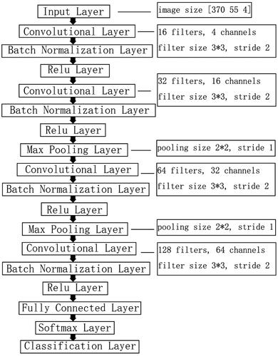
CNN consisted of feature extraction network and classification network. The framework of classification models was shown in Figure 2. A 18-layers CNN was used in the study, which consisted of input layer, convolutional layers, activation layers, batch normalization layers, pooling layers, fully connection layer, softmax layer and classification layer. Four convolutional layers and 2 max pooling layers were contained in the feature extraction network. The rectified linear unit (ReLU) activation function was used as activation function. According to the previous studies [29–33], we searched hyperparameter based on a number of different model designs for CNN, each of which was defined by the hyperparameter in Table 1. Other training options were as follow: maximum number of epochs were 20, initial learning rate was 0.001, mini batch size was 32.

Figure 2. Illustration of construction of deep learning networks. CNN consisted of feature extraction network and classification network. Four convolutional layers and 2 max pooling layers were contained in feature extraction network. In classification network, softmax function was employed for the final fully connected layer. The model of CNN combined with classifiers consisted of feature extraction network from CNN and classifiers network. Classifiers such as SVM, random forest or logistic regression can be found in classifiers network.

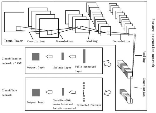
Table 1. Hyperparameters considered in CNN.

Hyperparameter	Value
Numbers of filters in the initial convolutional layer	8, 16
Filter size in convolutional layer	3*3, 4*4, 5*5
Stride of filter	1, 2, 4
Pooling size	2*2, 3*3
Gradient methods	SGDM, ADAM

SGDM: Stochastic gradient descent with momentum; ADAM: adaptive moment estimation.

As for model of CNN combined with machine learning classifier, SVM, random forest and logistic regression was employed as the last layer instead of fully connected layer, respectively (Figure 2). Hyperparameters of SVM and random forest were searched by Bayesian optimization. Linear model was used for logistic regression.

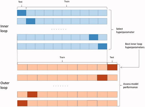
To mitigate against hyperparameter over-fitting or model selection bias, nested 10-fold cross-validation was used for selection of hyperparameter values and for measurement of classifying performance. The input data were divided into 10 folds for cross-validation as outer loop. For every outer loop, the training data were used to implement a 10-fold cross-validation, which was called inner loop. The inner loop aimed to optimize hyperparameter of the model. The parameters with best performance in inner loop were used to train models, and outer loop was used for performance assessment. The procedure of nested 10-fold cross-validation was shown in Figure 3.

Figure 3. Nested 10-fold cross-validation procedure for hyperparameter selection and model evaluation.

ROIs with size of 2 cm * 2 cm in acoustic nonlinearity map were used as input data. Data augmentation technique was used to enhance the size of sample and reduce the over-fitting problem. Each acoustic nonlinearity map had possibility of 50% to random cropping, left-right flipping, left rotation or up-down flipping.

Assessment of classification model and statistical analysis

Receiver operator characteristic (ROC) curve and area under curve (AUC) were used for estimating the probability of the correct prediction of liver fibrosis stages. Delong test was employed for comparisons of differences between different AUCs. The cutoff values with highest Youden Index was selected to calculate sensitivity, specificity, positive and negative likelihood ratios. All statistical tests were two sided, and p values less than 0.05 indicated statistical significance. The statistical analyses were performed using SPSS 20 and MedCalc 14.

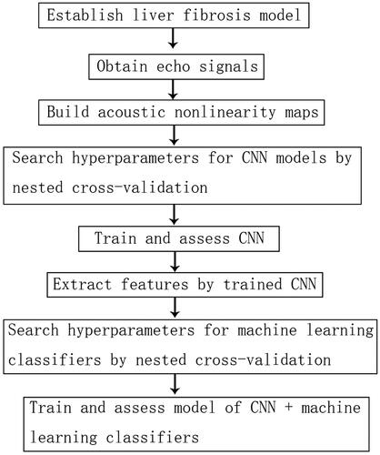
The basic flow chart of the study was displayed in Figure 4. Firstly, model of liver fibrosis was established. Once acoustic nonlinearity maps were built, we divided them into training data and testing data by nested 10-fold cross-validation. Inner loop of nested 10-fold cross-validation was used to select hyperparameter. Outer loop was used to train model and assess model performance. The features were extracted by trained CNN. Then, the classifiers were trained by the extracted features. Finally, the testing data set from outer loop was used to assess the diagnostic performance.

Figure 4. Flow chart of the study.

Result

Echo signal data and histological evaluation could be obtained in a total of 60 rabbits. Ten times of echo signals were acquired for each rabbit. A total of 600 acoustic nonlinearity maps were recorded. Twenty rabbits died in the process of experiment due to acute liver failure or other unknown causes. Fourteen of the 20 rabbits were died in early period of the experiment and the rest were died in later period. According to the evaluation of liver fibrosis, there were 10, 12, 13, 13, and 12 rabbits with fibrotic stage F0, F1, F2, F3 and F4, respectively.

The details of final CNN model were shown in Figure 5. The optimizer was stochastic gradient descent with momentum (SGDM). The kernel function used in SVM was linear and box constraint was 0.24. The maximal number of decision splits for random forest was 24 and the minimum number of leaf node was 116. The model of logistic regression was linear.

Figure 5. Structure of CNN in the study. The padding mode in each convolutional layer and pooling layer was ‘same’.

The accuracy, sensitivity, specificity, positive likelihood ratio and negative likelihood ratio for diagnosis of various stages of fibrosis were shown in Table 2. ROC curve was displayed in Figure 6. Model of CNN combined with SVM demonstrated the best diagnostic performance compared with all other methods for diagnosis of significant fibrosis (≥ F2), advanced fibrosis (≥F3) and cirrhosis (F4) and the differences of AUCs were all statistically significant (p < 0.05). The confusion matrixes were shown in Table 3. AUCs of CNN combined with SVM achieved 0.82, 0.88 and 0.90 for three stratifications, respectively, which were 0.04, 0.04 and 0.08 higher than these of CNN who showed the second highest AUCs. Other index to evaluate diagnostic performance including sensitivity, specificity and accuracy also demonstrated that CNN combined with SVM was the best model among these four models. CNN also showed good sensitivity and specificity predicting various fibrosis stages. Models using random forest or logistic regression did not show satisfactory efficiency with AUCs less than 0.7.

Figure 6. Comparison of receiver operating characteristic (ROC) curves among CNN, CNN + SVM, CNN + random forest and CNN + logistic regression. (A) ROC curve for classifying significant fibrosis (≥F2); (B) ROC curve for classifying advanced fibrosis (≥F3); (C) ROC curve for classifying cirrhosis (F4).

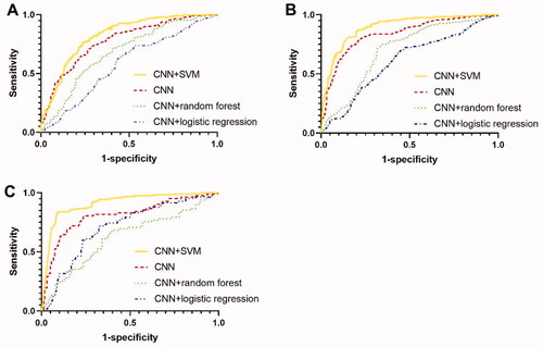
Table 2. Comparisons using different models of deep learning to classify liver fibrosis stages.

Classification model	AUC	Sensitivity	Specificity	Accuracy	LR+	LR−
Significant fibrosis (≥F2)
CNN	0.78	0.73	0.71	0.71	2.5	0.4
	(0.75–0.8)	(0.65–0.81)	(0.66–0.78)	(0.62–0.78)	(1.9–3.1)	(0.3–0.6)
CNN + SVM	0.82	0.83	0.66	0.75	2.4	0.3
	(0.80–0.84)	(0.79–0.89)	(0.56–0.76)	(0.71–0.85)	(1.8–3.0)	(0.2–0.6)
CNN + random forest	0.68	0.7	0.59	0.66	1.7	0.4
	(0.66–0.70)	(0.63–0.79)	(0.43–0.69)	(0.56–0.76)	(1.0–2.4)	(0.3–0.9)
CNN + logistic regression	0.57	0.68	0.5	0.61	1.4	0.6
	(0.55–0.59)	(0.60–0.74)	(0.51–0.59)	(0.51–0.69)	(1.2–1.7)	(0.3–0.8)
Advanced fibrosis (≥F3)
CNN	0.84	0.78	0.82	0.8	4.4	0.3
	(0.82–0.86)	(0.68–0.88)	(0.76–0.89)	(0.73–0.88)	(3.7–5.0)	(0.3–0.4)
CNN + SVM	0.88	0.8	0.86	0.84	5.7	0.2
	(0.86–0.90)	(0.72–0.87)	(0.81–0.91)	(0.79–0.88)	(4.8–6.6)	(0.1–0.4)
CNN + random forest	0.68	0.69	0.75	0.73	2.7	0.4
	(0.66–0.70)	(0.61–0.77)	(0.63–0.84)	(0.62–0.80)	(2.4–3.0)	(0.2–0.8)
CNN + logistic regression	0.57	0.7	0.54	0.6	1.6	0.6
	(0.54–0.60)	(0.61–0.78)	(0.36–0.66)	(0.53–0.73)	(1.0–2.4)	(0.3–0.7)
Cirrhosis (F4)
CNN	0.82	0.77	0.85	0.84	5.1	0.3
	(0.80–0.84)	(0.67–0.88)	(0.80–0.90)	(0.77–0.88)	(4.4–5.6)	(0.2–0.4)
CNN + SVM	0.9	0.83	0.92	0.9	10	0.2
	(0.88–0.92)	(0.78–0.88)	(0.89–0.95)	(0.87–0.93)	(8–12)	(0.2–0.3)
CNN + random forest	0.62	0.68	0.64	0.65	1.8	0.5
	(0.60–0.64)	(0.55–0.79)	(0.55–0.73)	(0.54–0.74)	(1.3–2.3)	(0.3–0.7)
CNN + logistic regression	0.7	0.71	0.69	0.70	2.3	0.4
	(0.67–0.73)	(0.56–0.86)	(0.59–0.79)	(0.60–0.80)	(1.7–2.9)	(0.3–0.6)

When applicable, statistical quantifications were displayed with 95% CI.

AUC of CNN + SVM or CNN was compared with the rest 3 models.

AUC: Area under curve; CNN: convolutional neural network; SVM: support vector machine; LR+: positive likelihood ratio; LR−: negative likelihood ratio.

Table 3. Confusion matrix.

CNN Significant fibrosis (≥F2)	Prediction results		Advanced fibrosis (≥F3)			Cirrhosis (F4)	Prediction results
				Prediction results
True results	<F2	≥F2	True results	<F3	≥F3	True results	<F4	F4
<F2	156	64	<F3	287	63	<F4	408	72
≥F2	103	277	≥F3	57	193	F4	28	92
CNN-SVM
Significant fibrosis (≥F2)			Advanced fibrosis (≥F3)			Cirrhosis (F4)
	Prediction results			Prediction results			Prediction results
True results	<F2	≥F2	True results	<F3	≥F3	True results	<F4	F4
<F2	143	77	<F3	301	49	<F4	442	38
≥F2	65	315	≥F3	50	200	F4	20	100
CNN-random forest
Significant fibrosis (≥F2)			Advanced fibrosis (≥F3)			Cirrhosis (F4)
	Prediction results			Prediction results			Prediction results
True results	<F2	≥F2	True results	<F3	≥F3	True results	<F4	F4
<F2	130	77	<F3	263	87	<F4	307	173
≥F2	114	266	≥F3	77	173	F4	38	82
CNN-logistic regression
Significant fibrosis(≥F2)			Advanced fibrosis (≥F3)			Cirrhosis (F4)
	Prediction results			Prediction results			Prediction results
True results	<F2	≥F2		<F3	≥F3		<F4	F4
<F2	110	110	<F3	189	161	<F4	341	139
≥F2	122	258	≥F3	75	175	F4	37	83

The overall diagnostic accuracy of CNN combined with SVM for ≥ F3 and F4 outperformed the diagnostic accuracy for significant fibrosis (AUC 0.88 and 0.90 vs 0.82). For diagnosis of ≥ F2, sensitivity and specificity also dropped. This phenomenon was also found in other models.

We also trained multi-class classification model to predict all the stages of fibrosis (from F0 to F4). Nevertheless, the accuracy of multi-class classification model was less than that of the two-class classification model. The respective result is shown in Table S1.

Discussion

In this study, deep learning models based on acoustic nonlinearity maps were used to estimate stages of liver fibrosis in rabbits with liver fibrosis. Acoustic nonlinearity maps were built using information extracted from echo signals. We found that the model of CNN and the model of CNN combined with SVM correctly staged liver fibrosis with high probability.

Following the extraction of features in CNN, the features can be input into classifiers such as SVM and random forest. In last two decades, the features of images were basically extracted by humanity using manual methods. Statistics features such as mean and standard deviation are known to be used in machine learning models. Chen et al. extracted statistics features from real-time elastography [34]. SVM, random forest and other machine learning classifiers in that study showed comparable performance with accuracy of 0.9 for cirrhosis. Li et al. extracted statistics and texture features from radio frequency data and B-mode images and demonstrated good performance of SVM and random forest with AUC of 0.85 [35]. In our study, SVM with features extracted by CNN showed AUC of 0.82, 0.88 and 0.90 to diagnose significant fibrosis, advanced fibrosis and cirrhosis, respectively. Although this result was comparable with other studies, the way to extract features in our study was fundamentally different from those studies.

A total of 4 models were evaluated in this study. CNN combined with SVM showed best diagnostic performance for liver fibrosis with AUC ranging from 0.82 to 0.90. Deep learning methods using ultrasound images, such as B-mode images or elastography, to diagnose liver fibrosis had been investigated in recent years [23,36]. A study conducted by Wang et al. employed CNN to analyze elastography images. AUCs for diagnosing significant fibrosis, advanced fibrosis and cirrhosis were 0.85, 0.98 and 0.97, respectively [23]. Lee et al. trained CNN with B-mode images and the AUC reached to 0.91 for cirrhosis [36]. The result was still close to our study despite the different input data.

In our study, the diagnostic performance for advanced fibrosis and cirrhosis was better than that for significant fibrosis. It is commonly seen that differentiating F0-F1 from F2-F4 is more challenging in previous studies [23,37]. It might be because that the heterogeneity of pathological features in stage ≥ F2 is more severe in stage ≥ F3 or F4. The heterogeneity decreases the accuracy not only in strategies of traditional ultrasound images but also deep learning methods. The accuracy of multi-class classification model was not satisfactory. A potential explanation for unsatisfactory result might be that there are overlaps of pathological features between adjacent fibrotic stages. Moreover, sample size is more insufficient if multi-class classification model is used. Nearly all the existing methods to non-invasively diagnose liver fibrosis are not accurate enough to distinguish between separate stages of fibrosis (F1 – F4) [3,38]. In clinical practice guidelines for liver fibrosis, significant fibrosis(> =F2), advanced fibrosis(> =F3) and cirrhosis(F4) are important end point, reflecting the prognosis and directing selection of treatment methods [3]. Hence, recognizing these three stages can also improve the routine clinical works.

AUC, sensitivity, specificity and accuracy displayed by CNN combined with SVM was better than that by CNN. The better performance of CNN-SVM in our investigation was in line with the findings of earlier studies [29,30,39,40]. We think that the better performance might be related with the small number of sample. According to other researches [29,41,42], although shortcoming of SVM is that its capabilities of deep feature extraction and data mining are insufficient, it has better generalization ability and can reduce the computational complexity. Therefore, SVM is more suitable for processing small sample data. In contrast, CNN required larger sample size to maximize its property.

There were several limitations in this study. Firstly, the sample size was limited. Although 600 maps were included and data was augmented by reversing and flipping images, it is not so much for training CNN which needs a large amount of imaging data. Further studies are required to prove the result. Secondly, the fibrotic liver specimens were obtained from rabbits and induced by CCL₄, which is different from clinic works. Besides the above limitations, the algorithm to obtain acoustic nonlinearity data and the models of deep learning needs to be further optimized. Lastly, it is difficult to explain the implication of features that CNN extracted. Therefore, the results are not explainable. To validate the efficiency of the methods in our study, a larger database is needed. Meanwhile, it would be more convincing if data from human liver were obtained.

Conclusion

A deep learning method based on acoustic nonlinear maps to diagnose liver fibrosis of rabbits was proposed in this study. Acoustic nonlinear maps were derived from echo signals. The deep learning models were helpful in classifying fibrosis stages. The model of CNN combined with SVM showed best performance to diagnose significant fibrosis, advanced fibrosis and cirrhosis and demonstrated potential for clinical generalization. The models still require further validation by larger size of data.

Disclosure statement

The authors declare that they have no known competing financial interests or personal relationships that could have appeared to influence the work reported in this paper.

Additional information

Funding

This study has received funding by National Natural Science Foundation, China No. 81671702.

References

- Dulai PS, Singh S, Patel J, et al. Increased risk of mortality by fibrosis stage in nonalcoholic fatty liver disease: systematic review and meta-analysis. Hepatology. 2017;65(5):1557–1565.
- Song J, Ma Z, Huang J, et al. Comparison of three cut-offs to diagnose clinically significant portal hypertension by liver stiffness in chronic viral liver diseases: a meta-analysis. Eur Radiol. 2018;28(12):5221–5230.
- EASL-ALEH. Clinical practice guidelines: non-invasive tests for evaluation of liver disease severity and prognosis. J Hepatol. 2015;63(1):237–264.
- Campana L, Iredale JP. Regression of liver fibrosis. Semin Liver Dis. 2017;37(1):1–10.
- Bedossa P, Carrat F. Liver biopsy: the best, not the gold standard. J Hepatol. 2009;50(1):1–3.
- Rockey DC, Caldwell SH, Goodman ZD, et al. Liver biopsy. Hepatology. 2009;49(3):1017–1044.
- McPherson S, Stewart SF, Henderson E, et al. Simple non-invasive fibrosis scoring systems can reliably exclude advanced fibrosis in patients with non-alcoholic fatty liver disease. Gut. 2010;59(9):1265–1269.
- Wai C-T, Greenson JK, Fontana RJ, et al. A simple noninvasive index can predict both significant fibrosis and cirrhosis in patients with chronic hepatitis C. Hepatology. 2003;38(2):518–526.
- Dietrich CF, Bamber J, Berzigotti A, et al. EFSUMB guidelines and recommendations on the clinical use of liver ultrasound elastography, update 2017 (long version). Ultraschall Med. 2017;38(4):e16–e47.
- Terrault NA, Bzowej NH, Chang K-M, et al. AASLD guidelines for treatment of chronic hepatitis B. Hepatology. 2016;63(1):261–283.
- Zarski J-P, Sturm N, Guechot J, et al. Comparison of nine blood tests and transient elastography for liver fibrosis in chronic hepatitis C: the ANRS HCEP-23 study. J Hepatol. 2012;56(1):55–62.
- Varray F, Basset O, Tortoli P, et al. Extensions of nonlinear B/a parameter imaging methods for echo mode. IEEE Trans Ultrason Ferroelectr Freq Control. 2011;58(6):1232–1244.
- van Sloun R, Demi L, Shan C, et al. Ultrasound coefficient of nonlinearity imaging. IEEE Trans Ultrason Ferroelectr Freq Control. 2015;62(7):1331–1341.
- Choi H, Woo P, Yeom J-Y, et al. Power MOSFET linearizer of a high-voltage power amplifier for high-frequency pulse-echo instrumentation. Sensors. 2017;17(4):764.
- Chen W, Wang P, Zhang Z, et al. Nonlinear ultrasonic imaging in pulse-echo mode using Westervelt equation: a preliminary research. Comput Assist Surg. 2019;24(sup2):54–61.
- Gong X, Zhang D, Liu J, et al. Study of acoustic nonlinearity parameter imaging methods in reflection mode for biological tissues. J Acoust Soc Am. 2004;116(3):1819–1825.
- Zhang D, Gong XF. Experimental investigation of the acoustic nonlinearity parameter tomography for excised pathological biological tissues. Ultrasound Med Biol. 1999;25(4):593–599.
- Nikoonahad M, Liu DC. Pulse-echo single frequency acoustic nonlinearity parameter (B/A) measurement. IEEE Trans Ultrason Ferroelectr Freq Control. 1990;37(3):127–134.
- Fatemi M, Greenleaf JF. Real-time assessment of the parameter of nonlinearity in tissue using “nonlinear shadowing”. Ultrasound Med Biol. 1996;22(9):1215–1228.
- Niel O, Bastard P. Artificial intelligence in nephrology: core concepts, clinical applications, and perspectives. Am J Kidney Dis. 2019;74(6):803–810.
- Nalepa J, Marcinkiewicz M, Kawulok M. Data augmentation for Brain-Tumor segmentation: a review. Front Comput Neurosci. 2019;13:83.
- Murray NM, Unberath M, Hager GD, et al. Artificial intelligence to diagnose ischemic stroke and identify large vessel occlusions: a systematic review. J Neurointerv Surg. 2020;12(2):156–164.
- Wang K, Lu X, Zhou H, et al. Deep learning radiomics of shear wave elastography significantly improved diagnostic performance for assessing liver fibrosis in chronic hepatitis B: a prospective multicentre study. Gut. 2019;68(4):729–741.
- Tajbakhsh N, et al. Convolutional neural networks for medical image analysis: full training or fine tuning? IEEE Trans Med Imaging. 2016;35(5):1299–1312.
- Sokolovsky M, Guerrero F, Paisarnsrisomsuk S, et al. Deep learning for automated feature discovery and classification of sleep stages. IEEE/ACM Trans Comput Biol Bioinform. 2020;17(6):1835–1845.
- Qiu T, Wang H, Song J, et al. Assessment of liver fibrosis by ultrasound elastography and contrast-enhanced ultrasound: a randomized prospective animal study. Exp Anim. 2018;67(2):117–126.
- Kuznetsov V. Equations of nonlinear acoustics. Sov Phys Acoust. 1971;16:467–470.
- Tjotta J, Tjotta S. Non-linear equations of acoustics, with application to parametric acoustic arrays. J Acoust Soc Amer. 1981;69(6):1644–1652.
- Gong W, Chen H, Zhang Z, et al. A novel deep learning method for intelligent fault diagnosis of rotating machinery based on improved CNN-SVM and multichannel data fusion. Sensors. 2019;19(7):1693.
- Wu H, Huang Q, Wang D, et al. A CNN-SVM combined model for pattern recognition of knee motion using mechanomyography signals. J Electromyogr Kinesiol. 2018;42:136–142.
- Paisarnsrisomsuk S, Ruiz C, Alvarez S. Improved deep learning classification of human sleep stages. 2020 IEEE 33rd International Symposium on Computer-Based Medical Systems (CBMS). 2020. p. 338–343.
- Chen Y-M, Chen YJ, Tsai Y-K, et al. Classification of human electrocardiograms by multi-layer convolutional neural network and hyperparameter optimization. IFS. 2021;40(4):7883–7891.
- Chou F-I, Tsai Y-K, Chen Y-M, et al. Optimizing parameters of multi-layer convolutional neural network by modeling and optimization method. IEEE Access. 2019;7:68316–68330.
- Chen Y, Luo Y, Huang W, et al. Machine-learning-based classification of real-time tissue elastography for hepatic fibrosis in patients with chronic hepatitis B. Comput Biol Med. 2017;89:18–23.
- Li W, Huang Y, Zhuang B-W, et al. Multiparametric ultrasomics of significant liver fibrosis: a machine learning-based analysis. Eur Radiol. 2019;29(3):1496–1506.
- Lee JH, Joo I, Kang TW, et al. Deep learning with ultrasonography: automated classification of liver fibrosis using a deep convolutional neural network. Eur Radiol. 2020;30(2):1264–1273.
- Li Y, Huang Y-S, Wang Z-Z, et al. Systematic review with meta-analysis: the diagnostic accuracy of transient elastography for the staging of liver fibrosis in patients with chronic hepatitis B. Aliment Pharmacol Ther. 2016;43(4):458–469.
- Thiele M, Madsen BS, Procopet B, et al. Reliability criteria for liver stiffness measurements with real-time 2D shear wave elastography in different clinical scenarios of chronic liver disease. Ultraschall Med. 2017;38(6):648–654.
- Navaneeth B, Suchetha M. PSO optimized 1-D CNN-SVM architecture for real-time detection and classification applications. Comput Biol Med. 2019;108:85–92.
- You W, Shen C, Guo X, et al. A hybrid technique based on convolutional neural network and support vector regression for intelligent diagnosis of rotating machinery. Adv Mech Eng. 2017;9(6):168781401770414.
- Liu R, Yang B, Zio E, et al. Artificial intelligence for fault diagnosis of rotating machinery: a review. Mech Syst Sig Process. 2018;108:33–47.
- Shen T, Jiang J, Li Y, et al. Decision supporting model for one-year conversion probability from MCI to AD using CNN and SVM. Annu Int Conf IEEE Eng Med Biol Soc. 2018. 2018;2018:738–741.