Optimal definitions for computing HKA angle in caos: an in-vitro comparison study

Abstract

The goal of this study was to assess and compare the precision and accuracy of nine and seven methods usually used in Computer Assisted Orthopedic Surgery (CAOS) to estimate respectively the Knee Center (KC) and the Frontal Plane (FP) for the determination of the HKA angle (HKAA). An in-vitro experiment has been realized on thirteen cadaveric lower limbs. A CAOS software application was developed and allowed the computation of the HKAA according to these nine KC and seven FP methods. The precision and the accuracy of the HKAA measurements were measured. The HKAA precision was highest when the FP is determined using the helical method. The HKAA accuracy was highest using the helical approach to determine the FP and either the notch or the tibial spines to determine the KC. This study shows that the helical approach to determine the FP and either the notch or the middle of tibia spines are the combinations that provide both a good enough accuracy and precision to estimate the HKA.

Keywords:

• Knee center
• frontal plane
• HKA
• CAOS

1. Introduction

Hip-Knee-Ankle HKA angle (HKAA) is an essential parameter in orthopedics which describes lower limb alignment. HKAA is defined as a two-dimensional (2D) angle in frontal plane formed between the mechanical axes of individual tibia and femur and in neutrally aligned limb, this angle is 180° [1,2]. HKAA is used in a significant number of surgical procedures, mainly associated to the lower limb axis control or correction. The HKAA must therefore be accurately determined since it significantly influences in-surgery decisions such as selecting cutting planes, implant positioning and can thus affect post-operative results [3,4].

Studies have shown that Computer Assisted Orthopedic Surgery (CAOS) can reduce the complications for the interventions requiring an accurate measurement of the HKAA [5–8]. Although there is a consensus in the literature to obtain the frontal HKAA on anteroposterior (AP) radiographs [1,9], several approaches have been applied in CAOS. The HKAA measurement relies on both the localization of the three lower limb joint centers (hip, ankle, and knee) and the determination of the frontal plane (FP). Thus, defining three centers and one plane are of prime importance in determining the lower limb alignment and the HKAA. The hip center (HC) and the ankle center (AC) are computed using well-established kinematic techniques, respectively, by acquiring the center of rotation of the circumduction motion of the hip [10–12], and by localizing the middle of the medial and lateral malleolus of the ankle [13]. However, multiple methods exist to determine both the knee center (KC) and the FP and to date there is no single study to report the efficacy of the methods used.

KC and FP determination methods can be classified into two approaches: morpho-functional approach and anatomical approach [14]. Anatomical approaches rely on the localization of specific anatomical landmarks whereas morpho-functional approaches rely on the knee kinematics. There exist at least nine techniques to determine KC and at least seven techniques to determine FP in current CAOS systems. Each of these techniques were implemented based on the familiarity and surgical sequences followed and adapted by various surgeons around the world. The accuracy and precision of CAOS systems to determine specific KC and FPs and to study the impact either on the HKAA measurement or on the final implant placement has been reported using either simulations [15,16], or mechanical test benches [7,17–19] or cadaveric specimens [5,18]. Two authors [20,21] have analyzed the intra and inter observer errors for localizing anatomical landmarks. Both studies were performed on only one cadaveric specimen and did not assess the influence on the HKAA measurement. Two studies have evaluated the precision and accuracy of the HKAA determined with one morpho-functional approach [22,23]. All these studies were performed using only one of the methods of determination of KC and FP and comparison of all the available methods together was therefore not possible.

The goal of this study is to assess and compare the precision and the accuracy of nine and seven methods usually used in CAOS to localize respectively the KC and the FP for the determination of the HKAA.

2. Materials AND methods

2.1. Cadaveric specimen and CAOS system

Thirteen cadaveric full lower limb specimens were used in this study. Each specimen was checked by an expert for avoiding any abnormalities that can be regarded as contraindications for the methods performed. None of the specimens had osteoarthritis. A CAOS system was constructed which was composed of a NDI POLARIS SPECTRA optical camera (NORTHERN DIGITAL®, Ontario, Canada), a computer with a processing unit Intel (R) Core (TM) 2 Duo (2.53 GHz and 4 Go RAM), two passive optical markers, and a digitizer equipped with an optical marker (NORTHERN DIGITAL^®, Ontario, Canada). Although accuracy information provided by the manufacturers are dependent on their own measurement protocols [24], this optical camera had, according to the manufacturer, a root mean square (RMS) accuracy of 0.35 mm.

2.2. Data acquisition and processing

Optical markers were placed on the diaphysis of tibia and femur using bone pins to track the bones (Figure 1). For determining the HC, AC, KC and FP, an inhouse software application was developed and installed on the CAOS system. Following data were acquired with the system:

Figure 1. Optical markers attached on the femur and the tibia.

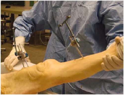
1. Hip circumduction: A circumduction motion of the femur was performed around the pelvis while keeping the knee in extension. HC corresponds to the center of rotation of this motion and was computed using the pivoting algorithm [25].

2. Ankle landmarks: The medial and lateral malleolus were digitized with regards to the tibial optical markers and the center of both malleoli was determined as AC.

3. Flexion-extension motion of the knee: Tibia was flexed from 0° to 90° and back. The positions and rotations of the tibial optical markers were recorded with respect to the femoral optical markers during the motion.

4. Femoral epicondyles before dissection: The medial and lateral femoral epicondyles were digitized with respect to the femoral optical markers before dissection of the skin.

5. Femoral epicondyles after dissection: The medial and lateral femoral epicondyles were digitized with respect to the femoral optical markers after dissection of the skin.

6. Distal condyles of the femur: The most distal points of the medial and lateral condyles were digitized with respect to the femoral optical markers.

7. Posterior condyles of the femur: The most posterior points of the medial and lateral femoral condyles were digitized with respect to the femoral optical markers.

8. Center of the femoral notch: The center of the notch was digitized with respect to the femoral optical marker set.

9. Tibial spines: The vertices of the medial and lateral tibial spines were digitized with respect to the tibial optical marker set.

10. Tibial intercondylar eminence: The center of the tibial eminence between both the tibial spines was digitized with respect to the tibial optical marker set.

The entire data acquisition was conducted in two parts. For part one, data were acquired for steps one to four above and this process was repeated for five times. At the beginning of part two, each knee joint was kept at 30° flexion and a parapatellar medial arthrotomy was performed to access the anterior aspect of the knee joint by flipping the patella on the lateral side using soft tissue retractors. Skin was removed around the femoral epicondylar region to expose the bone. Data were acquired for steps five to ten above and the process was also repeated for five times.

2.3. KC, FP and HKAA determination

Nine KCs were computed according to the following definitions (Figure 2):

Figure 2. Definitions of the knee center explained on a schematic.

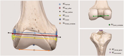
(1) KC_helical: Middle of the segment joining medial and lateral points belonging to the mean rotation axis estimated with the helical method which is based on the estimation of instantaneous screw axis (ISA) [26]; (2) KC_circle: Middle of the segment joining medial and lateral points belonging to the rotation axis estimated with the circle method which computes a mean circle describing, during the knee motion, the positions of the tibial markers with respect to the femoral markers [26]; (3) KC_notch: Center of the femoral notch as digitized [27]; (4) KC_{distal_condyles}: Center of the segment joining the most distal points of the medial and lateral condyles of the femur; (5) KC_{post_condyles}: Center of the segment joining the most posterior points of the medial and lateral condyles of the femur; (6) KC_{epi_before}: Center of the segment joining medial and lateral femoral epicondyles before removal of the skin; (7) KC_{epi_after}: Center of the segment joining medial and lateral femoral epicondyles after removal of skin; (8) KC_{tibial_spines}: Middle of the segment joining both the tibial spines [28]; (9) KC_eminence: Tibial intercondylar eminence as digitized [28].

The FP was defined as the plane containing the femoral axis joining the HC and KC and lying parallel to a medio-lateral vector passing through the KC. Seven FPs were computed according to the following definitions of the medio-lateral vector:

(1) FP_helical: Vector joining medial and lateral points belonging to the mean rotation axis estimated with the helical method; [26] (2) FP_circle: Vector joining medial and lateral points belonging to the rotation axis estimated with the circle method [26]; (3) FP_{post_condyles}: Vector joining the most posterior points of the medial and lateral condyles of the femur; (4) FP_{distal_condyles}: Vector joining the most distal points of the medial and lateral condyles of the femur; (5) FP_{epi_before}: Vector formed between both femoral epicondyles before removal of the skin; (6) FP_{epi_after}: Vector formed between both femoral epicondyles after removal of the skin; (7) FP_{tibial_spines}: Vector formed between both tibial spines;

For determining the 2 D HKA, tibia mechanical axis was projected onto each FP definition. The HKAA value was reported relative to 180° with positive HKAA value representing valgus knee and negative HKAA value representing varus knee.

2.4. Evaluation of precision and accuracy

2.4.1. KC precision

The KC precision was computed for all the KC definitions and was defined as a deviation from mean value of KC from five repeated measures: $${\mathit{Precision}}_{KC}\left(i,j\right)=\mathrm{ }\mathit{distance}({\overline{KC}}_i,{KC}_{i,\mathrm{ }j})$$ Where:

• $\mathit{distance}\left(a,b\right)$ was the 3D Euclidean distance between two points $a$ and $b;$

• ${\overline{KC}}_i$ was the mean value KC of the cadaveric lower limb i (i = 1–13);

• ${KC}_{i,\mathrm{ }j}$ was the KC acquired during the j^th experiment (j = 1–5) of the cadaveric lower limb i.

2.4.2. HKAA precision

The HKAA precision was computed for each combination of the KC and FP definitions and was defined as: $${\mathit{Precision}}_{\mathit{HKA}}(i,j)=\mathrm{ }\mathit{angle}({\overline{\mathit{HKA}}}_i,{\mathit{HKA}}_{i,j})$$ Where:

• $\mathit{angle}\left(a,b\right)$ was the angle between two HKAA $a$ and $b;$

• ${\overline{\mathit{HKA}}}_i\mathrm{ }$ was the average HKAA of the cadaveric lower limb i (i = 1 to 13);

• ${\mathit{HKA}}_{i,j}\mathrm{ }$ was the HKAA computed during the j^th experiment (j = 1 to 5) of the cadaveric lower limb i.

2.4.3. HKAA accuracy

The accuracy of the HKAA was computed for all combinations of KC and FP definitions with respect to a ground truth HKAA (HKA_{Ground_Truth}) computed from the assumptions of two authors made by (1) Moreland et al. [9] who considered that the HKA is defined on anteroposterior X-ray radiographs as the angle between the femoral axis joining the hip center and the notch, and the tibial axis joining the ankle center and the midpoint of both tibial spines, and (2) Minoda et al. [29] who considered that the lateral radiograph i.e. the sagittal view has to be acquired so that the posterior edges of the medial and lateral femoral condyles have to be aligned. HKA_{Ground_Truth} was therefore the average angle from the five acquisitions between the femoral axis joining the hip center and the notch, and the FP projection of the tibial axis joining the ankle center and the midpoint of both tibial spines. This FP was defined as the plane containing the femoral axis and lying parallel to the average medio-lateral vector from the five acquisitions passing through both posterior condyles. The accuracy of HKAA was defined as: $${\mathit{Accuracy}}_{\mathit{HKA}}(i,j)=\mathrm{ }\mathit{angle}({\mathit{HKA}}_{\mathit{Ground}\_\mathit{Truth}\mathrm{ }i},{\mathit{HKA}}_{i,j})$$ Where:

• $\mathit{angle}\left(a,b\right)$ was the angle between two HKAA $a$ and $b;$

• ${\mathit{HKA}}_{\mathit{Ground}\_\mathit{truth}\mathrm{ }i}\mathrm{ }$ was the HKA_{Ground_Truth} angle of the cadaveric lower limb i (i = 1–13);

• ${\mathit{HKA}}_{i,j}\mathrm{ }$ was the HKAA computed during the j^th experiment (j = 1–5) of the cadaveric lower limb i.

2.4.4. Statistical analysis

Mean and Standard-deviations (SD) were calculated for both HKA precision and accuracy of all FP and KC combinations. As we expected means values close to 0, the comparisons were therefore made between SD only as we defined as clinically relevant the methods having the sum (Mean + SD) inferior to 1°. We aimed to be able to find a difference between two SD of 0.75 with a statistical power of 80%. Therefore, we needed to include 13 cadavers (N = 13). Variances were compared using F-tests with α equal to 0.05. The statistical analysis was realized with MedCalc Statistical Software version (MedCalc Software, Ostend, Belgium; http://www.medcalc.org).

3. Results

3.1. KC precision

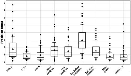
In the Figure 3, the KC precision was plotted as a boxplot for each KC definition. Mean precision values ranged from 0.8 mm to 2.9 mm with highest precision observed in determining KC_circle, KC_{tibial_spines} and KC_eminence and lowest precision observed in determining KC_{epi_before}. The value of outliers was highest in KC_helical and KC_{epi_before}. Among the morpho-functional approaches, KC_circle had the highest precision whereas among the anatomical approaches, KC_eminence was highest.

Figure 3. Boxplot of precision for nine definitions of the Knee Centers. The middle line represents the median, the box extends from the lower to the upper quartile, and the vertical line extends from the first decile to the ninth decile. Values which are inferior or superior to respectively the first and the ninth deciles are represented by separated points. Solid triangles in each box represent the mean precision values.

3.2. HKAA precision

HKAA precision is shown in the Table 1. In this table, the results of the noninvasive approaches, i.e. approaches which do not require incisions to reach anatomical landmarks and to compute HKAA, are highlighted in gray. FP and KC combinations having the sum (Mean + SD) inferior to 1° were highlighted in green. The HKAA precision was highest with the combinations of KC_{distal_condyles} - FP_helical and was lowest with the combination of KC_helical - FP_{tibial_spines}. For noninvasive approaches, the combination of KC_circle - FP_circle had highest precision (0.03°±1.00).

Table 1. HKA precision (mean ± SD, (min–max)) in degrees according to the KC and the FP definitions.

	FPhelical	FPcircle	FPepi_before	FPdistal_condyles	FPpost_condyles	FPepi_after	FPtibial_spines
KChelical	−0.05 ± 0.65	−0.10 ± 1.18	−0.22 ± 1.94	0.11 ± 0.82	0.22 ± 0.96	−0.23 ± 1.00	−1.00 ± 3.53
	(−3.58–1.13)	(−3.23–5.04)	(−3.83–5.75)	(−1.59–4.45)	(−2.11–3.31)	(−2.53–2.05)	(−16.12–5.31)
KCcircle	−0.05 ± 0.51	0.03 ± 1.00	−0.22 ± 1.93	0.14 ± 0.93	0.10 ± 1.43	−0.21 ± 0.82	−0.60 ± 2.93
	(−2.96–0.89)	(−3.17–5.35)	(−3.68–5.88)	(−1.73–5.32)	(−2.42–3.58)	(−1.79–1.68)	(−13.69–4.75)
KCepi_before	−0.05 ± 0.58	0.22 ± 1.64	−0.24 ± 2.14	0.25 ± 1.52	0.31 ± 2.21	−0.24 ± 0.92	−0.10 ± 2.40
	(−3.33–0.96)	(−3.78–5.43)	(−4.15–6.24)	(−2.02–7.33)	(−4.74–3.29)	(−2.10–1.51)	(−13.83–5.24)
KCnotch	−0.06 ± 0.58	0.02 ± 1.04	−0.15 ± 2.33	0.18 ± 1.12	−0.08 ± 1.67	−0.02 ± 1.15	−0.43 ± 2.37
	(−3.66–1.14)	(−3.70–5.55)	(−4.28–6.34)	(−1.97–6.09)	(−2.63–3.70)	(−2.32–2.88)	(−10.71–3.80)
KCdistal_condyles	−0.00 ± 0.91	−0.44 ± 1.96	−0.12 ± 2.06	0.46 ± 2.01	0.16 ± 2.08	−0.22 ± 0.99	−0.68 ± 4.43
	(−3.55–3.91)	(−3.84–5.62)	(−4.01–6.16)	(−2.48–8.22)	(−4.75–3.18)	(−2.54–1.85)	(−18.31–8.00)
KCpost_condyles	−0.21 ± 1.05	0.06 ± 1.68	0.07 ± 1.98	0.29 ± 1.63	0.10 ± 2.34	0.29 ± 1.39	−0.96 ± 5.08
	(−3.70–2.44)	(−3.91–5.38)	(−3.27–4.91)	(−2.17–7.41)	(−4.29–4.33)	(−2.53–3.09)	(−18.06–12.50)
KCepi_after	−0.06 ± 0.52	−0.42 ± 1.99	−0.34 ± 2.17	0.43 ± 2.12	0.44 ± 2.18	−0.16 ± 0.87	−0.10 ± 2.20
	(−3.13–0.90)	(−6.54–4.56)	(−4.32–6.44)	(−2.46–8.88)	(−7.98–3.02)	(−1.86–1.42)	(−12.74–5.31)
KCtibial_spines	−0.10 ± 0.81	0.05 ± 1.63	0.04 ± 1.99	0.22 ± 1.26	−0.07 ± 1.88	0.35 ± 1.34	−0.28 ± 3.06
	(−5.04–1.39)	(−3.26–4.67)	(−3.64–5.44)	(−1.80–6.49)	(−2.75–4.03)	(−3.33 − 2.04	(−13.63–4.28)
KCeminence	−0.23 ± 1.30	0.13 ± 1.73	0.11 ± 2.06	0.25 ± 1.27	−0.02 ± 2.04	0.37 ± 1.62	−0.26 ± 3.03
	(−3.61–3.07)	(−3.85–5.01)	(−3.22–5.01)	(−2.84–6.66)	(−3.16–4.54)	(−3.78–3.48)	(−13.66–4.71)

FP and KC combinations having the sum (Mean + SD) inferior to 1° are highlighted in green. Noninvasive methods are in gray.

3.3. HKAA accuracy

HKAA accuracy is shown in the Table 2. In this table, the results of the noninvasive approaches are also highlighted in gray. FP and KC combinations having the sum (Mean + SD) inferior to 1° were highlighted in green. HKAA accuracy was best with the combination of KC_helical - FP_{post_condyles} (-0.01°±1.65) and was worst with the combination of KC_{post_condyles} – FP_{tibial_spines} (-1.16°±5.82). For noninvasive approaches, combination of KC_{epi_before} – FP_{epi_before} resulted in highest accuracy (0.06°±2.28).

Table 2. HKA accuracy (mean ± SD, (min–max)) in degrees according to the KC and the FP definitions.

	FPhelical	FPcircle	FPepi_before	FPdistal_condyles	FPpost_condyles	FPepi_after	FPtibial_spines
KChelical	−0.36 ± 0.91	−0.46 ± 1.40	−0.20 ± 2.11	0.42 ± 1.20	−0.01 ± 1.65	0.09 ± 1.40	0.05 ± 3.33
	(−2.56–1.55)	(−3.49–2.32)	(−8.39–3.92)	(−1.81–4.50)	(−6.39–3.73)	(−3.46–3.68)	(−13.39–8.82)
KCcircle,	−0.52 ± 0.71	−0.36 ± 1.17	−0.20 ± 2.12	0.39 ± 1.23	0.02 ± 1.65	0.12 ± 1.34	−0.12 ± 3.04
	(−2.01–2.55)	(−3.47–2.19)	(−8.37–3.82)	(−1.82–4.40)	(−6.39–3.81)	(−3.06–3.64)	(−11.78–8.31)
KCepi_before	−0.32 ± 1.05	−0.11 ± 1.75	0.06 ± 2.28	0.29 ± 1.59	0.28 ± 2.00	0.55 ± 1.35	−0.18 ± 2.73
	(−3.05–2.15)	(−3.85–3.09)	(−8.57–4.60)	(−4.67–3.04)	(−7.34–5.65)	(−2.45–6.31)	(−12.16–7.62)
KCnotch	−0.16 ± 0.68	0.07 ± 1.08	−0.11 ± 2.27	0.25 ± 1.18	−0.06 ± 1.70	0.24 ± 1.24	−0.34 ± 2.77
	(−2.57–2.21)	(2.54–3.49)	(−8.43–6.44)	(−2.16–4.55)	(−6.43–4.73)	(−3.05–4.31)	(−9.71–7.64)
KCdistal_condyles	−0.09 ± 1.04	0.15 ± 1.64	0.42 ± 2.26	0.68 ± 1.96	0.38 ± 1.98	0.85 ± 1.39	−0.27 ± 4.00
	(2.82–2.51)	(−2.95–4.03)	(−7.97–4.49)	(−5.01–6.68)	(−7.34–5.65)	(−2.40–6.41)	(−15.37–10.58)
KCpost_condyles	0.32 ± 1.31	0.14 ± 1.77	0.26 ± 2.23	0.16 ± 1.57	−0.04 ± 2.15	0.57 ± 1.53	−1.16 ± 5.82
	(−3.11–3.64)	(−3.35–4.13)	(−7.68–6.92)	(−3.62–4.68)	(−7.34–5.99)	(−3.88–7.19)	(−18.44–10.61)
KCepi_after	−0.23 ± 1.22	0.03 ± 2.26	0.25 ± 2.35	0.36 ± 2.11	0.64 ± 1.90	0.66 ± 1.35	−0.14 ± 2.65
	(−3.63–1.55)	(−3.00–4.13)	(−9.58–5.10)	(−4.90–7.89)	(−8.48–5.97)	(−2.83–6.10)	(−11.33–6.26)
KCtibial_spines	−0.06 ± 0.84	−0.05 ± 1.64	−0.02 ± 2.06	0.11 ± 1.27	−0.15 ± 1.85	0.36 ± 1.35	−0.02 ± 2.99
	(−2.56–1.92)	(−3.65–2.42)	(−8.62–4.29)	(−2.70–4.95)	(−6.79–4.57)	(−3.85–5.23)	(−11.55–8.75)
KCeminence	0.02 ± 1.32	−0.36 ± 2.09	−0.13 ± 2.12	−0.10 ± 1.37	−0.33 ± 1.95	0.09 ± 1.54	−0.02 ± 2.98
	(−1.57–3.01)	(−4.03–2.73)	(−8.03–4.22)	(−4.28–2.47)	(−6.75–4.96)	(−4.03–4.93)	(−11.12–9.14)

FP and KC combinations having the sum (Mean + SD) inferior to 1° are highlighted in green. Noninvasive methods are in gray.

3.4. Statistical analysis

p-Values regarding SD for the accuracy are presented in the Table 3.

Table 3. p-Values between FP and KC combinations and either the FP_helical – KC_notch (top) and FP_helical – KC_{tibial_spines} (down) for the accuracy (NA: Not Applicable).

	FPhelical	FPcircle	FPepi_before	FPdistal_condyles	FPpost_condyles	FPepi_after	FPtibial_spines
KChelical	0.33	*	*	0.06	*	*	*
	0.79	0.09	*	0.23	*	0.09	*
KCcircle,	0.88	0.07	*	*	*	*	*
	0.57	0.26	*	0.20	*	0.12	*
KCepi_before	0.15	*	*	*	*	*	*
	0.45	*	*	*	*	0.11	*
KCnotch	NA	0.12	*	0.07	*	*	*
	0.47	0.40	*	0.25	*	0.19	*
KCdistal_condyles	0.16	*	*	*	*	*	*
	0.47	*	*	*	*	0.09	*
KCpost_condyles	*	*	*	*	*	*	*
	0.14	*	*	*	*	*	*
KCepi_after	*	*	*	*	*	*	*
	0.21	*	*	*	*	0.11	*
KCtibial_spines	0.47	*	*	*	*	*	*
	NA	*	*	0.17	*	0.11	*
KCeminence	*	*	*	*	*	*	*
	0.13	*	*	0.10	*	*	*

Only non-significant results are presented (p > 0.05), significant results are represented with the (*) symbol.

4. Discussion

This study successfully evaluated the precision of determining KC and the precision and the accuracy to measure HKAA using most frequently used definitions of the KC and the FP from the literature. To the knowledge of the authors, this is the first study to report the precision and accuracy of the HKAA determination using various techniques and thus would prove as a guiding tool for the development of CAOS solutions for knee surgical procedures. The results of this study not only recommend the KC-FP definitions to use but also provide an error map for different combinations.

The precision of the KC localization was directly linked to the well identification of the anatomical landmarks, which was in accordance with the literature [20,21]. When the landmarks were not salient (for instance KC_{epi_before}) or situated in the middle of a large bony surface (such as KC_{distal_condyles} or KC_{post_condyles}), the KC localization was comparatively less precise. The KC localization based either on the tibial spines or on the tibial eminence were the most precise methods as they were distinctly identifiable and palpable during the surgical procedure. Furthermore, noninvasive approaches such as KC_helical and KC_{epi_before} resulted in less precision.

The precision of HKAA measurement was very influenced by the FP definition, making FP_{tibial_spines} the worst plane of choice and FP_helical the best plane of choice. Thus, for a precise measurement of the HKAA, determination of the medio-lateral vector plays a major role, which was highlighted by this study. Previous studies have warranted the need to standardize the method for the HKAA measurement realized from an AP x-ray radiographs to avoid the influence of the lower limb rotation [2,30]. The current study enhances this understanding by providing a comparison for different FP selection methods and thus can be effectively used as a guide. In some clinical applications such as high tibial osteotomy, the anatomical landmarks are not visible, reachable or exposed. In such cases, FP and KC must be determined using noninvasive methods, either morpho-functional approaches (helical or circle) or cutaneous methods (localization of both femoral epicondyles on the skin). This study found that the helical method was more precise than the cutaneous methods.

As for the HKAA precision, HKAA accuracy was also dominated by FP_helical definition, confirming thus the quality of this definition. If we consider that the clinical requirement to estimate the HKA have to be superior to 1° since, depending on the surgery, the acceptable range for the HKAA after Total Knee Arthroplasty is 180° ± 3° [31], and between 183° and 186° for High Tibia Osteotomy (HTO), it is important to note that the morpho-functional helical approach to determine the FP and either KC_notch, or KC_{tibial_spines} can provide HKAA accuracy superior to this requirement. CAOS systems can therefore be developed using morpho-functional helical approach only if needed. This is a major finding for minimally invasive knee procedures that still have to rely on HKAA measures for their successful outcomes (for e.g. HTO). In many clinical applications such as total or unilateral knee arthroplasty, the acquisition of anatomical landmarks can be realized via the incision. In this case, the FP is usually determined with either the epicondyles, the posterior condyles, or the distal condyles. The KC can be defined as either KC_notch, KC_{distal_condyles}, KC_{post_condyles}, KC_{epi_after}, the KC_{tibial_spines} or the KC_eminence. From the results of this study, it can be can observed that any combination of these configurations lead to HKAA errors inferior to 1°, even if some configurations have large SD. The combinations FP_{distal_condyles}-KC_notch, FP_{distal_condyles}-KC_eminence, and the FP _{epi_after} with either, KC_notch, KC_{distal_condyles}, KC_{epi_after}, and KC_{tibial_spines} provide the best accuracy with a moderate SD (i.e. < 1.5°).

Finally, there were several limitations associated to this study. First, the assessment of the HKAA accuracy was done with respect to one gold standard we computed from two assumptions made by Moreland et al. [9] and Minoda [29]. However, this gold standard is still today controversial. Second, the inter-observer variability was not evaluated in this study and has also been little studied in the literature. Goleski et al. have assessed the inter-observer variability of one cutaneous morpho-functional approach to estimate the varus-valgus for High Tibia Osteotomy (HTO) and have found that inter-observer variability was only fair [5]. Jenny et al. have found that navigation allows a high precision to measure the mechanical axis with an intra- and inter-observer variation of only 0.1° ± 0.7° using an anatomical approach for TKA. Conclusions about the inter-observer variabilities are therefore still today controversial and mainly depend on two criteria (1) the good identification of landmarks and (2) the used approach to estimate the HKA [5,20,21]. Third, the specimens didn’t have any abnormalities in the knee. Tthe knee flexion-extension motion could be disturbed by the presence of either Knee Osteoarthritis (KOA), flexion contracture or hyper-laxity, influencing thus the rotation axis computation of the morpho-functional approaches, and impacting the estimation of both the KC and the FP. The presence of osteophytes, very common in case of KOA, could also influence the landmarks localization used to determine the KC or the FP because of the possible presence of small bony outgrowths on the regions of interest. It would be therefore very relevant in the future to deeply investigate the impact of these pathologies onto both the precision and the accuracy of the approaches allowing the HKA estimation. And fourth, the accuracy of the localizer could have also a direct impact on the accuracy of both the landmarks and the flexion/extension motion acquisitions, and thus on the accuracy of the HKA determination. Our experiment has been done with a NDI POLARIS SPECTRA optical camera, but it would be necessary to further analyze the influence of several impacting effects onto the accuracy camera such as the warm-up or the quality of the calibration that could occur, as well as others camera models having different localization technology that could be used during surgery.

5. Conclusions

This in-vitro experiment on 13 cadaveric specimen shows that the helical approach to determine the FP and either the notch or the middle of tibia spines to determine the KC are the combinations that provide both a good enough accuracy and precision to estimate the HKA.

Acknowledgements

We would like to also thanks the PLaTIMed platform for the access to the anatomical lab (www.platimed.fr).

Disclosure statement

No potential conflict of interest was reported by the author(s).

Additional information

Funding

This work was supported by the French National Research Agency under the “Investissements d’Avenir” program [ref. ANR-17-RHUS-0010].

References

- Cherian JJ, Kapadia BH, Banerjee S, et al. Mechanical, anatomical, and kinematic axis in TKA: concepts and practical applications. Curr Rev Musculoskelet Med. 2014;7(2):89–95.
- Cooke TD, V, Sled EA, Scudamore RA. Frontal plane knee alignment: a call for standardized measurement. J Rheumatol. 2007;34:1796–1801.
- Callaghan JJ, O’rourke MR, Saleh KJ. Why knees fail: lessons learned. J Arthroplasty. 2004;19(4 Suppl 1):31–34.
- Liau JJ, Cheng CK, Huang CH, et al. The effect of malalignment on stresses in polyethylene component of total knee prostheses–a finite element analysis. Clin Biomech (Bristol, Avon). 2002;17(2):140–146.
- Goleski P, Warkentine B, Lo D, et al. Reliability of navigated lower limb alignment in high tibial osteotomies. Am J Sports Med. 2008;36(11):2179–2186.
- Mason JB, Fehring TK, Estok R, et al. Meta-analysis of alignment outcomes in computer-assisted total knee arthroplasty surgery. J Arthroplasty. 2007;22(8):1097–1106.
- Pitto RP, Graydon AJ, Bradley L, et al. Accuracy of a computer-assisted navigation system for total knee replacement. J Bone Joint Surg Br. 2006;88(5):601–605.
- Weber P, Crispin A, Schmidutz F, et al. Improved accuracy in computer-assisted unicondylar knee arthroplasty: a meta-analysis. Knee Surg Sports Traumatol Arthrosc. 2013;21(11):2453–2461.
- Moreland JR, Bassett LW, Hanker GJ. Radiographic analysis of the axial alignment of the lower extremity. J Bone Joint Surg Am. 1987;69(5):745–749.
- Dib Z, Dardenne G, Poirier N, et al. Detection of the hip center in computer-assisted surgery: an in vitro assessment study. IRBM. 2013;34(4–5):319–321.
- Lopomo N, Sun L, Zaffagnini S, et al. Evaluation of formal methods in hip joint center assessment: an in vitro analysis. Clin Biomech. 2010;25(3):206–212.
- Dardenne G, Dib Z, Poirier N, et al. What is the best hip center location method to compute HKA angle in computer-assisted orthopedic surgery? In silico and in vitro comparison of four methods. Orthop Traumatol Surg Res. 2019;105(1):55–61.
- Siston RA, Daub AC, Giori NJ, et al. Evaluation of methods that locate the center of the ankle for computer-assisted total knee arthroplasty. Clin Orthop Relat Res. 2005;439:129–135.
- Siston RA, Giori NJ, Goodman SB, et al. Surgical navigation for total knee arthroplasty: a perspective. J Biomech. 2007;40(4):728–735.
- Robinson M, Eckhoff DG, Reinig KD, et al. Variability of landmark identification in total knee arthroplasty. Clin Orthop Relat Res. 2006;442:57–62.
- Schlatterer B, Linares J-M, Chabrand P, et al. Influence of the optical system and anatomic points on computer-assisted total knee arthroplasty. Orthop Traumatol Surg Res. 2014;100(4):395–402.
- Brin YS, Livshetz I, Antoniou J, et al. Precise landmarking in computer assisted total knee arthroplasty is critical to final alignment. J Orthop Res. 2010;28(10):1355–1359.
- Fuiko R, Kotten B, Zettl R, et al. [The accuracy of palpation from orientation points for the navigated implantation of knee prostheses]. Orthopade. 2004;33(3):338–343.
- Lustig S, Fleury C, Goy D, et al. The accuracy of acquisition of an imageless computer-assisted system and its implication for knee arthroplasty. Knee. 2011;18(1):15–20.
- Perrin N, Stindel E, Roux C. BoneMorphing versus freehand localization of anatomical landmarks: Consequences for the reproducibility of implant positioning in total knee arthroplasty. Comput Aided Surg. 2005;10(5–6):301–309.
- Yau WP, Leung A, Chiu KY, et al. Intraobserver errors in obtaining visually selected anatomic landmarks during registration process in nonimage-based navigation-assisted total knee arthroplasty: a cadaveric experiment. J Arthroplasty. 2005;20(5):591–601.
- Chang C-W, Yang C-Y. Kinematic navigation in total knee replacement—experience from the first 50 cases. J Formos Med Assoc. 2006;105(6):468–474.
- Jenny J, Boeri C, Picard F, et al. Reproducibility of intra-operative measurement of the mechanical axes of the lower limb during total knee replacement with a non-image-based navigation system. Comput Aided Surg. 2004;9(4):161–165.
- Elfring R, de la Fuente M, Radermacher K. Assessment of optical localizer accuracy for computer aided surgery systems. Comput Aided Surg. 2010;15(1–3):1–12.
- Siston RA, Delp SL. Evaluation of a new algorithm to determine the hip joint center. J Biomech. 2006;39(1):125–130.
- Gil JD, Stindel E, Guillard G, et al. Detection of the functional knee center using the mean helical axis: application in computer assisted high tibial osteotomy. In: 2004 2nd IEEE Int. Symp. Biomed. Imaging Macro to Nano (IEEE Cat No. 04EX821). Vol. 2, IEEE; n.d. p. 1557–60.
- Bonnin M, Chambat P. La gonarthrose: traitement chirurgical: de l'arthroscopie à la prothèse. Springer; 2006.
- Cazalis P. Diagnostic et traitement d’un genou douloureux. Editions techniques. Encycl Méd Chir. 1994;14–325. https://www.em-consulte.com/article/8293/diagnostic-et-traitement-d-un-genou-douloureux
- Minoda Y, Kobayashi A, Iwaki H, et al. Sagittal alignment of the lower extremity while standing in Japanese male. Arch Orthop Trauma Surg. 2008;128(4):435–442.
- Cooke TDV, Sled EA. Optimizing limb position for measuring knee anatomical axis alignment from standing knee radiographs. J Rheumatol. 2009;36(3):472–477.
- Ritter MA, Faris PM, Keating EM, et al. Postoperative alignment of total knee replacement. Its effect on survival. Clin Orthop Relat Res. 1994;153–156.