A shape-partitioned statistical shape model for highly deformed femurs using X-ray images

Abstract

To develop a patient-specific 3 D reconstruction of a femur modeled using the statistical shape model (SSM) and X-ray images, it is assumed that the target shape is not outside the range of variations allowed by the SSM built from a training dataset. We propose the shape-partitioned statistical shape model (SPSSM) to cover significant variations in the target shape. This model can divide a shape into several segments of anatomical interest. We break up the eigenvector matrix into the corresponding representative matrices for the SPSSM by preserving the relevant rows of the original matrix without segmenting the shape and building an independent SSM for each segment. To quantify the reconstruction error of the proposed method, we generated two groups of deformation models of the femur which cannot be easily represented by the conventional SSM. One group of femurs had an anteversion angle deformation, and the other group of femurs had two different scales of the femoral head. Each experiment was performed using the leave-one-out method for twelve femurs. When the femoral head was rotated by 30°, the average reconstruction error of the conventional SSM was 5.34 mm, which was reduced to 3.82 mm for the proposed SPSSM. When the femoral head size was decreased by 20%, the average reconstruction error of the SSM was 4.70 mm, which was reduced to 3.56 mm for the SPSSM. When the femoral head size was increased by 20%, the average reconstruction error of the SSM was 4.28 mm, which was reduced to 3.10 mm for the SPSSM. The experimental results for the two groups of deformation models showed that the proposed SPSSM outperformed the conventional SSM.

Keywords:

• Statistical shape model
• 3D reconstruction
• femur modeling

Introduction

Three-dimensional (3D) models of human anatomical structures, such as bones and organs, are useful for health professionals to diagnose the conditions of patients in a clinical situation. Computed tomography (CT) and magnetic resonance image (MRI) datasets are needed to build 3D models of human anatomical structures, but acquiring CT and MRI data is expensive, and it is rarely covered by insurance. CT scanning also exposes a patient to radiation. Recently, statistical shape models (SSMs), originally developed by Cootes et al. [1] for image processing and analysis, have been widely used to model 3D anatomical structures [2]. SSMs have shaped reconstruction approaches, and an SSM, which acquires statistical information such as a mean shape and significant components of variation using principal component analysis (PCA), can adapt to a range of variations in the anatomical structure, allowed by the linear span of the training examples.

Considerable progress in the development of SSMs for patient-specific 3D reconstruction from 2D X-ray images has recently been made. It is useful to obtain patient-specific 3D models of specific anatomical structures from 2D X-ray images, which are readily available from most clinics. This type of patient-specific 3D modeling is also useful for designing implants, planning surgical operations, examining medical operation results, and developing computer-aided surgical navigation systems [2,3]. Chan et al. [4] used ultrasound images instead of X-ray images for 3D/2D matchings. The procedure of 3D reconstruction using SSM can be divided into two major aspects: registration and feature matching between 3D models and 2D images, and the optimization of the shape parameters of the SSM. Fleute et al. [5] performed non-rigid 3D/2D registration using a generalized version of the iterative closest point (ICP) algorithm, and they applied 3D reconstruction using SSM to the distal femur. Benameur et al. [6] proposed a different type of 3D/2D registration, in which a deformable template matching method was employed to change the model template of scoliotic vertebrae to be matched to 2D X-ray images. SSM reconstruction was achieved by comparing the outer boundaries of a template to the boundaries of 2D images and minimizing an energy function designed by the researchers. Fleute et al. and Benameur et al. focused on calculating exact pose parameters, while Zheng et al. [7] placed more emphasis on building 3D/2D correspondence with X-ray contour points, and projected 2D points from a 3D model by introducing a symmetric injective nearest-mapping operator and a 2D thin-plate splines-based deformation, thereby improving the accuracy of the 3D reconstruction of SSM. Rajamani et al. [8] introduced a new joint cost function for sparse data to obtain better 3D reconstruction results, which was an approach also adopted by Zheng et al. [7].

Recent studies have used simulated X-ray images or digitally reconstructed radiographs (DRRs). Instead of the 3D model vertices being projected, the 3D model is voxelized, and DRRs are obtained using ray-casting, where intensity information is extracted and used in various ways [9]. Yao et al. [10] voxelized a 3D model derived from SSM to produce DRRs and achieved 3D/2D registration using DRR and X-ray images. Yu et al. [11] suggested a fully automatic 3D/2D reconstruction of the proximal femur that incorporated intensity information from a DRR. Cerveri et al. [12] tried to improve the 3D/2D reconstruction accuracy of the distal femur based on SSM for possible use as a personalized surgical instrument. They experimented on a CT knee dataset of 100 patients with cartilage damage. In a recent study, Cerveri et al. adopted the basic idea of their previous paper and performed various experiments concerning the relationship between joint instability and modes of variation of eigenvectors [13]. Youn et al. [14] focused on an iterative method for self-calibration, pose estimation, and optimization using lateral (LAT), and anterior-posterior (AP) X-ray views, which were used for the 3D reconstruction of the femur. The salient feature of Kim’s work [15] was the use of a convolutional neural network (CNN) for automatic feature analysis, with which they constructed 3D models from front-view lower limb X-ray images. Given biplanar real X-ray images, Kasten et al. [16] presented an end-to-end CNN, which was trained using a deep learning algorithm based on DRRs to achieve the 3D reconstruction of knee joints instead of using SSM. O’Connor et al. [17] analyzed the influence of the reconstruction accuracy of 2D input images when there was rotation around the femoral axis. These researchers also found [18] that the error in femoral height measurement was important and could lead to inappropriate surgical planning when femoral rotation was unknown.

The advantage of using SSMs is that they can adapt to reasonable variations of a shape in a class of shapes. However, when the shape parameters of the SSM change, the overall shape changes to fit the given shape, because the modes of eigenvectors in the SSM formulation are redistributed by the shape parameters and eigenvectors and are not related to specific parts or landmarks of a shape [19]. The shape changes caused by the redistribution of eigenvectors are sometimes not the changes that users intend to produce. Even though the shape change can be achieved by SSM within representations obtained by the eigenvector matrix derived from the training dataset, SSM does not allow for selective change to only a specific part of a shape. Zhang et al. [20] obtained automatically defined regions that were similar to anatomical features of the femur, enforced the correspondence of such features across the training dataset, and assembled fitted region meshes to obtain the region-based SSM (rSSM). The rSSM performed better than regular SSMs, although the rSSM involved complicated steps. Lüthi et al. [21] proposed Gaussian process morphable models (GPMMs), in which shape variations were modeled using a Gaussian process represented by basis functions derived from the Karhunen-Loève expansion of a sample covariance kernel. Whereas an SSM is described by eigenfunctions from the covariance matrix through PCA analysis, and the shape variation of an SSM is represented using the linear span of the training dataset, the shape variation of a GPMM can be defined by a general Gaussian process, which provides a robust model against artifacts or noise. More sophisticated modeling is also achievable if multiscale models or posterior models related to reference and target landmarks of the dataset are used. Recently, Fouefack et al. [22] proposed dynamic multi-object-Gaussian process modeling (DMO-GPM) based on GPMM, in which they showed that multiple objects and their pose variations could be learned using a Gaussian process for analyzing the shape and motion of a human shoulder joint.

In this paper, we propose a shape-partitioned SSM (SPSSM) applied to the 3D reconstruction of the femur. This method allows the partitioning of the shape into several segments of anatomical interest. We show that it is possible to change the shape parameters of SSMs independently for each segment by simply breaking up the eigenvector matrix into the corresponding representative matrices, each of which preserves the relevant rows of the original matrix. We also derived a mathematical formulation for the SPSSM. When we apply the conventional SSM to the partitioned segments, we should build SSM through the PCA algorithm for each segment and also estimate the initial poses of the segments. The advantage of the proposed method over the existing method is that it avoids the repeated procedure of building separate SSMs for the partitioned segments. We built two deformation models that represent possible deformations of the femur. It was found that deformation models were not accurately reconstructed by conventional SSMs using X-ray images, whereas the deformation models were more faithfully reconstructed using X-ray images by the SPSSMs. The usefulness of the SPSSM was evaluated in terms of the reconstruction error.

Materials and methods

Statistical shape models

The SSM described by Cootes et al. constructs a statistical model from given shape samples, thus allowing the adaptation of the model to geometrical shape variations [1]. Assuming that s training shapes are available to construct an SSM, a training shape is represented by a vector ${\mathit{x}}_i, i\in \{1,\dots ,s\},$ of which the elements are d corresponding landmarks across the training shapes. At the time of SSM implementation, the landmarks corresponding to the linked 3D coordinates of a group of vertices are included in the segment. The mean shape $\overline{\mathbf{x}}$ of the training, shapes are given by: (1) $$\overline{\mathbf{x}}=\frac{1}{s}\sum _{i=1}^s{\mathbf{x}}_i$$(1)

The covariance matrix is given by: (2) $$\mathbf{S}=\frac{1}{s-1}\sum _{i=1}^s\left({\mathbf{x}}_i-\overline{\mathbf{x}}\right){\left({\mathbf{x}}_i-\overline{\mathbf{x}}\right)}^T$$(2)

A shape $\mathbf{x}$ can be described through PCA as: (3) $$\mathbf{x}=\overline{\mathit{x}}+\mathbf{\Phi }\mathbf{b}$$(3) in which $\overline{\mathit{x}}$ is the mean shape, $\mathbf{\Phi }$ is the matrix of eigenvectors representing the modes of the shape variations in the training shape data, and $\mathbf{b}$ is the vector of shape parameters that weight the eigenvectors in parameter space. The number of eigenvectors t is equal to or smaller than the number of training shapes if we select t eigenvectors corresponding to the t largest eigenvalues. The eigenvectors are represented by ${\mathit{\varphi }}_i, i\in \left\{1,\dots ,t\right\}, t\le s,$ and we have $\mathbf{\Phi }=\{{\mathit{\varphi }}_1 {\mathit{\varphi }}_2\dots {\mathit{\varphi }}_t\}.$ The $\mathbf{b}$ in Equation (3)(3) $$\mathbf{x}=\overline{\mathit{x}}+\mathbf{\Phi }\mathbf{b}$$(3) works as a control parameter, and it controls the overall shape of $\mathbf{x}.$

Shape-partitioned statistical shape model

Vector $\mathbf{b}$ has t shape parameters. As an element ${\mathit{b}}_{\mathit{i}}$ in $\mathbf{b}$ becomes larger, the weight of the corresponding eigenvector becomes larger and the overall shape changes because of the larger ${\mathit{b}}_{\mathit{i}}$ according to Equation (3)(3) $$\mathbf{x}=\overline{\mathit{x}}+\mathbf{\Phi }\mathbf{b}$$(3) . The problem is that we cannot focus on altering only a specific part of a shape. To change a specific part of a shape, rather than the overall shape, we propose to partition the shapes according to our region of interest, so that only a partitioned segment can change its geometrical shape, while the other segments remain unchanged. A set of landmarks in the k^th segment of the shape is denoted as ${\mathit{p}}_k,$ and the number of segments is assumed to be K. First, $\overline{\mathbf{x}}$ can be divided into K components given by: (4) $$\overline{\mathbf{x}}={\overline{\mathbf{x}}}_{{\mathbf{p}}_1}+{\overline{\mathbf{x}}}_{{\mathbf{p}}_2}+\cdots +{\overline{\mathbf{x}}}_{{\mathbf{p}}_K}$$(4)

Let the i^th element of ${\overline{\mathbf{x}}}_{{\mathbf{p}}_{\mathit{k}}}$ be ${{\left(x_i\right)}_P}_k,$ and let the i^th element of $\overline{\mathbf{x}}$ be $\overline{x_i}.$ Then we have: $${{\left(x_i\right)}_{\mathbf{P}}}_k=\{\begin{array}{l}\overline{x_i} l_i\in {\mathbf{p}}_k\\ 0 l_i\notin {\mathbf{p}}_k\end{array},i\in (1,\dots ,d)$$

Similarly, we divide matrix $\mathbf{\Phi }$ into K separate partitions as follows: (5) $$\mathbf{\Phi }={\mathbf{\Phi }}_{{\mathbf{p}}_1}+{\mathbf{\Phi }}_{{\mathbf{p}}_2}+\cdots +{\mathbf{\Phi }}_{{\mathbf{p}}_{\mathit{K}}}$$(5) in which ${\mathbf{\Phi }}_{{\mathbf{p}}_{\mathit{k}}}$ is a partial $\mathbf{\Phi }$ with respect to ${\mathit{p}}_k.$ Let the (i, j)^th element of $\mathbf{\Phi }$ be ${\mathit{\varphi }}_{\mathit{i},\mathit{j}},$ and the (i,j)th element of ${\mathbf{\Phi }}_{{\mathbf{p}}_{\mathit{k}}}$ be defined by: $${{\left({\mathit{\varphi }}_{\mathit{i},\mathit{j}}\right)}_{\mathbf{P}}}_k=\{\begin{array}{l}{\mathit{\varphi }}_{\mathit{i},\mathit{j}} l_i\in {\mathbf{p}}_k\\ 0 l_i\notin {\mathbf{p}}_k\end{array},i\in (1,\dots ,d)$$

If partitioned ${\overline{\mathbf{x}}}_{{\mathbf{p}}_{\mathit{k}}}$ and ${\mathbf{\Phi }}_{{\mathbf{p}}_{\mathit{k}}}$ are used instead of $\overline{\mathbf{x}}$ and $\mathbf{\Phi },$ it is possible to change the resulting reconstructed shape by changing ${\mathbf{b}}_{\mathit{k}},$ which corresponds to the kth segment of a shape. To obtain ${\mathbf{\Phi }}_{{\mathbf{p}}_{\mathit{k}}}$ is quite simple, since the rows of ${\mathbf{\Phi }}_{{\mathbf{p}}_{\mathit{k}}}$ related to the landmark ${\mathit{p}}_k$ are retained, and the remaining rows are filled with zeros. The reconstructed shape ${\mathit{x}}_r$ is obtained by simply adding the partitioned shapes. The ${\mathit{x}}_{{\mathit{p}}_{\mathit{k}}}$ is constructed using ${\overline{\mathbf{x}}}_{{\mathbf{p}}_{\mathit{k}}}$ and ${\mathbf{\Phi }}_{{\mathbf{p}}_{\mathit{k}}},$ which results in a shape that is related to the landmarks belonging to ${\mathit{p}}_k.$ We have: (6) $${\mathit{x}}_{{\mathit{p}}_{\mathit{k}}}={\overline{\mathbf{x}}}_{{\mathbf{p}}_{\mathit{k}}}+{\mathbf{\Phi }}_{{\mathbf{p}}_{\mathit{k}}}{\mathit{b}}_{\mathit{k}}$$(6)

The final reconstructed shape ${\mathit{x}}_r$ is defined as: $${\mathbf{x}}_r={\mathbf{x}}_{{\mathbf{p}}_1}+{\mathbf{x}}_{{\mathbf{p}}_2}+\dots +{\mathbf{x}}_{{\mathbf{p}}_K}$$ $$=\sum _{k=1}^K{\overline{\mathbf{x}}}_{{\mathbf{p}}_{\mathit{k}}}+\sum _{k=1}^K{\mathbf{\Phi }}_{{\mathbf{p}}_k}{\mathbf{b}}_k$$ (7) $$=\overline{\mathit{x}}+\sum _{k=1}^K{\mathit{\Phi }}_{{\mathit{p}}_{\mathit{k}}}{\mathit{b}}_{\mathit{k}}$$(7)

The vector b, with t elements relating to the corresponding eigenvectors, works as a weighting factor since each element of b weights the importance of the eigenvector. If b is changed, the overall shape is changed, according to Equation (3)(3) $$\mathbf{x}=\overline{\mathit{x}}+\mathbf{\Phi }\mathbf{b}$$(3) . However, in our case, we focus on one specific segment of a shape, for example, the kth segment related to ${\mathit{p}}_k.$ From that segment, we calculate a new ${\mathbf{b}}_{\mathit{k}}$ by adapting the model to a specific example, which then changes the shape according to Equation (7)(7) $$=\overline{\mathit{x}}+\sum _{k=1}^K{\mathit{\Phi }}_{{\mathit{p}}_{\mathit{k}}}{\mathit{b}}_{\mathit{k}}$$(7) . Similarly, we can change the other ${\mathbf{b}}_{\mathit{k}}$ vectors at the same time. This means that we have k shape vectors ${\mathbf{b}}_{\mathit{k}}$ instead of one, which provides us with considerable freedom to match the SSM to real examples, especially when deformation occurs to a specific part of a shape.

Workflow of the 3D reconstruction with SPSSM

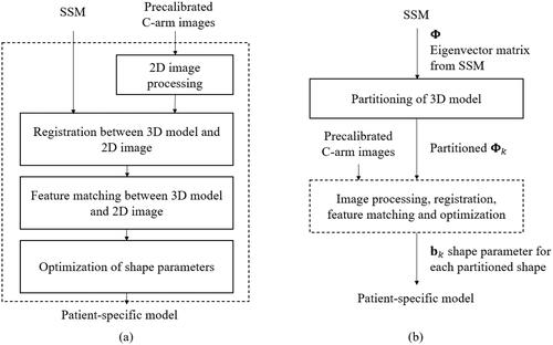
Recently, SSMs have been used to adapt 3D models to one or more specific examples. We applied SSMs to the patient-specific reconstruction of a given femur model, in which a 3D model represented by an SSM is changed to a more accurate model by matching the model to specific C-arm images, which are X-ray images obtained using a C-arm device. The procedure is summarized in Figure 1(a). To make the reconstruction process more flexible and accurate, SPSSM can be employed instead of the conventional SSM when the target example to be adapted shows severe partial-shape variation with respect to the training datasets. Here, the shapes are partitioned, and for each segment of a shape, we obtain a partitioned eigenvector matrix ${\mathbf{\Phi }}_{{\mathbf{p}}_{\mathit{k}}}$ which enables us to use the separate shape parameter vector ${\mathbf{b}}_{\mathit{k}}.$ Only one of the segments ${\mathbf{b}}_{\mathit{k}}$ works as a controlling parameter to optimize a segment, and it can take on a new value to improve the femur model. The new ${\mathbf{b}}_{\mathit{k}}$ produces a more patient-specific model which is matched to the 2D C-arm images of a patient. The detailed image processing steps, 3D/2D registration, feature matching, and optimization steps are summarized in Figure 1, and they will be elaborated on in the following sections.

Figure 1. (a) Configuration of the conventional SSM for femur reconstruction. (b) From the conventional SSM, the new SPSSM is constructed and used to produce a more patient-specific reconstruction of a 3D femur model.

Boundary descriptions of C-arm images

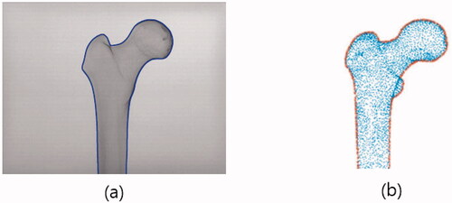
Our intent was to match pre-calibrated C-arm images to the projected 2D points of vertices of a 3D femur model described by an SSM. For this kind of matching, the boundary description of an object was adopted for its simplicity in image processing and advantage in speed. We note that the C-arm images only cover the part of a femur that is of clinical interest, that is, the proximal part or the distal part. Figure 2(a) shows the proximal part of a femur and its detected boundary.

Figure 2. (a) C-arm images and extracted outer boundary shown as a blue curve. (b) Vertex points are shown as blue dots, and the vertices of their outer boundary are extracted and shown as red dots.

3D/2D registrations

To match a 3D femur surface model with 2D C-arm images, a feature matching method was adopted. The first step is the estimation of the pose parameters, which reflect the changes in translation, rotation, and scale between 2D images and a 3D model. The second step is the projection of the 3D vertices of a femur model onto the 2D C-arm image plane. Based on the intrinsic parameters of the C-arm calibration procedure, a virtual X-ray source is assumed, and the vertices in the 3D models are projected onto 2D image points using a projection matrix consisting of intrinsic and extrinsic parameters as its elements. The X-ray imaging system is analyzed using a regular pinhole camera model [23]. The intrinsic parameters are determined by the focal length of the camera, the width and height of a pixel on the projection plane, and the principal points, whereas the extrinsic parameters are determined by the rotation and translation between the camera coordinates and the world coordinates [23,24]. The third step is to extract the outer vertices from the projected vertices, as shown in Figure 2(b). Procrustes analysis on these boundary points and the boundary points obtained from C-arm images are used to estimate the pose parameters between the 2D images and the 3D models.

Feature matching between 3D models and 2D images

After the pose parameters have been obtained, it is possible to align the 2D image with respect to the outer boundary points projected from the 3D model. The shapes of the 2D images are sometimes slightly different from the projected images of the model, so we cannot use simple matching, which pairs the two nearest points. Instead, we choose a starting point after the alignment, and we follow the boundary points of the two boundary images. We choose a pair of points that are located at roughly the same distance from a starting point after length normalization, and label them as corresponding points.

Optimization

To reconstruct the femur model, the shape parameters need to be updated after the presentation of the 2D images, which leads to the modification of x in Equation (3)(3) $$\mathbf{x}=\overline{\mathit{x}}+\mathbf{\Phi }\mathbf{b}$$(3) . We assume that there are N corresponding points in the previous feature matching procedure. Let $I_i=(x_i y_i)$ be the i^th point in the 2D images for i = 1,…, N, which corresponds to the i^th projected point $I_i^P=\left(x_i^P y_i^P\right)={\mathit{T}}_{\mathit{proj}}{\mathbf{x}}^{\mathbf{i}},$ where ${\mathbf{x}}^{\mathbf{i}}$ is the i^th matched shape vector and ${\mathit{T}}_{\mathit{proj}}$ is a projection matrix. Many methods have been used to define the cost function for fitting 2D image points and 3D model points. One category is based on the least-squares method, which minimizes the distances between 2D boundary points and matched projected points. The cost function E we used is defined as: (8) $$E\left(\mathbf{b}\right)={{\omega }_{1}E}_{\mathit{fit}}+{\omega }_2{E}_r={\omega }_1\sum _{i=1}^N\mathit{dis}{t}^2\left(I_i,I_i^P\right)+{\omega }_2\sum _{j=1}^m\frac{b_j}{{\sigma }_j}$$(8) in which dist($I_i,I_i^P$) is the Euclidean distance between two matched points. Here, the parameters ${\omega }_1$ and ${\omega }_2$ weigh the relative importance of two error terms, usually on the condition that ${\omega }_1+{\omega }_2=1.$ $E_{\mathit{fit}}$ is a fitting error term, and $E_r$ is a regularization term, which improves the convergence behavior [8]. Here, ${\sigma }_j$ is a weighting parameter for $b_j,$ which is the j^th element of b. We assume that the m largest eigenvalues are used in the optimization. The optimization using the interior-point algorithm [25], which is available in the Optimization Toolbox of MATLAB, has been performed to update the shape parameters using the cost function. This algorithm is chosen since it allows for imposing limitations on the magnitude of the shape parameters. The constraints we used are $-3\sqrt{{\lambda }_i}\le b_i\le 3\sqrt{{\lambda }_i},$ where ${\lambda }_i$ is i^th the eigenvalue of the covariance matrix S and $b_i$ is the i^th shape parameter. 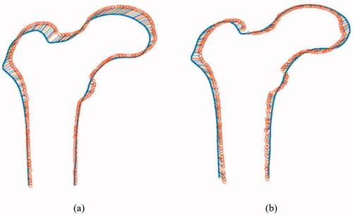These limitations are chosen since it was reported that $b_i$ over the training, data lies within three standard deviations of the mean [1]. Typical results for the optimization between two boundary points are shown in Figure 3. Figure 3(a and b) show the matching results before and after optimization.

Figure 3. Matching between the 2 D boundary points and projected points of the 3 D model vertices before optimization (a) and after optimization (b). A pair of matched points are linked by a line. After optimization, the red dots are rearranged, which results in lower cost, as shown clearly in (b).

Experimental results

Experimental setting

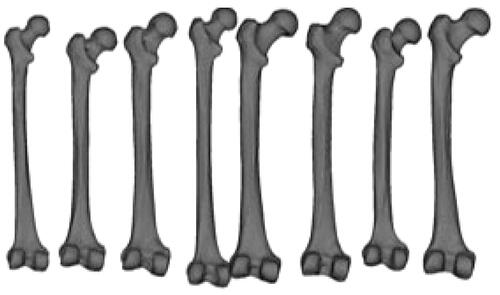
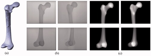
In our study, we used 12 commercial physical models of femur bone made from adult cadaver bones or real femur samples. We processed CT images of the bones to construct 3D surface models for building the SSM. The open-source 3D slicer [26] was used to convert 2D slice images into 3D surface mesh models. A mesh consists of triangle-shaped elements with three vertices. To build an SSM in 3D space, we used 9,871 ordered vertices defining meshes that correspond to their 3D coordinates across all models. Samples of the 3D surface models of the femurs are shown in Figure 4. The 2D femur images were introduced to make the SSM more patient-specific, and at least two X-ray images taken by C-arm from different viewing angles were used to adapt the 3D SSM. Two images separated by 30˚ were obtained. Some studies have used two orthogonal views separated by a 90˚, but we used a 30˚, because it is more practical in a clinical situation to use a small angle [7]. The images had a resolution of 1240 × 960 pixels, and the source-to-center distance was 600 mm. C-arm calibration [23,24] was used to estimate the intrinsic parameters of the C-arm, which will be used in the 3D/2D registration.

Figure 4. Samples of 3 D femur surface models were constructed from the CT images used in the experiments.

To evaluate the usefulness of the proposed SPSSM for the personalization of an SSM to the C-arm images of a patient, we devised two experiments on femur models. Twelve femurs were used, and the leave-one-out method [27] was used for cross-validation of the SSMs. One femur was chosen as the target to test the patient-specific reconstruction of SSMs or SPSSMs, while the remaining femurs were used to build SSMs. An SSM can change its shape via new shape parameters, thereby resembling the shape of a target. For healthy patients, a conventional SSM can be expected to perform reasonably well when it is adapted to the patient since the degree of variation in deformation for a patient is not very severe. We employed highly deformed models as targets based on the leave-one-out approach, and we used these deformed targets to evaluate the performance of the conventional SSM and the proposed SPSSM in terms of the reconstruction error. We built two types of deformed models. The first experiment involved the deformation of the femoral anteversion angle. In femur fracture reduction, it is occasionally necessary to test the degree of correctness of the estimation of the anteversion angle to restore a dislocation or a fracture of a femur to the normal position. Such a deformation model is especially useful for patients whose anteversion angles are so wide that it is difficult to build a useful reconstruction model using conventional SSM. The second model involved head scale deformation. The shapes or sizes of parts of a femur can vary from person to person. It can be theoretically or practically valuable to evaluate the way in which SSM can be adapted to the variation in the shape of a specific part of a femur. For this, we introduced a scale deformation model of the femoral head by changing the size of a femoral head, and we observed the capability of SSM to correctly restore the head size. There is no definite rule for selecting K since the number of segments is chosen by observing the local variations of the object and determining which part should be modified to obtain a better description of the local deformation.

In summary, we have presented a series of experiments on two types of deformations. The first experiment was concerned with the deformation of femoral anteversion angle and the resulting reconstruction errors, where one reconstruction result was obtained using X-ray images for SSM and SPSSM, and another result was obtained using DRRs for SSM and SPSSM. The second experiment was concerned with the scale deformation of the femoral head and the resulting reconstruction errors. We obtained two sizes of femoral heads by increasing or decreasing the scale by 20%. The reconstruction errors were obtained using DRRs for the SSM and SPSSM.

Results of deformation of femoral anteversion angle

The anteversion angle is formed by two lines: the line on the distal condylar axis, and the line obtained by projecting the line on the neck-shaft axis onto the horizontal plane. The anteversion angle roughly represents the rotation of the femoral neck with respect to the shaft [28]. We constructed a 3D deformation model in which the neck of the original femur was further rotated by 30˚ around the shaft of the femur in the counterclockwise direction, as shown in Figure 5(a). A series of C-arm images were captured for all the femur bone models. These images were used as 2D images to be matched with projected points from the 3D model. Since various models of deformation in the femur cannot easily be found in the market, and we could not obtain C-arm images directly from the deformed model, we reordered C-arm images from the normal model depending on the anteversion angle deformation. The two images in the upper row of Figure 5(b) show the proximal part, and the two remaining figures show the distal parts. For the reconstruction of 3D models by SSM, we used two views of C-arm images. For example, the two images in the first column in Figure 5(b) were employed for 3D/2D matchings. Since two views are required for 3D reconstruction, we introduced a different set of views, separated by 30˚, in the C-arm setting, as shown in the second column of Figure 5(b). During the process of building conventional SSMs and the proposed SPSSMs, the mean shape ($\overline{\mathit{x}}$) and the matrix of eigenvectors ($\mathbf{\Phi }$ or ${\mathbf{\Phi }}_{{\mathbf{p}}_{\mathit{k}}}$) had already been obtained, as described in the previous section, and the two views of C-arm images obtained from the deformed model in the anteversion angle were also available. For SPSSM, we first needed to divide the femur into two segments. We assumed a horizontal plane located midway along the length of the femur, by which the femur is split into two parts. Each part of the femur underwent the reconstruction procedure described below.

Figure 5. (a) Deformed 3 D model in which the deformation of the anteversion angle is 30˚. This deformed target was generated from the original No.10 femur. (b) C-arm images for the proximal and distal parts. The first column corresponds to C-arm images with a 0˚ view angle, whereas the second column corresponds to C-arm images with a 30˚ view angle. (c) Corresponding DRR images were obtained from the deformation model.

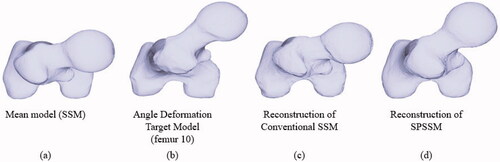
The first step was to reconstruct a new shape from the new shape parameters after 3D/2D registration, 3D/2D feature matching, and optimization, as previously detailed. The newly reconstructed shapes were evaluated in terms of point-to-surface error, which is generally used to measure the reconstruction error. We calculated the distances from the vertices of the reconstructed model to the surfaces of the target deformation model, and we used the root mean square (RMS) of the distance to represent the reconstruction error. One typical example which represents the shape reconstruction results of the deformed femur model is shown in Figure 6 for SSM and SPSSM. Figure 6(a) shows the mean model of the shape, and Figure 6(b) shows the target shape due to angle deformation, which is common in both cases. The shape reconstructed using the conventional SSM is shown in Figure 6(c), while the result reconstructed by the SPSSM is shown in Figure 6(d). The rotation deformation was not solved by using SSM, and its reconstruction result looks similar to the shape of the original mean model, while the rotation of the femoral head reconstructed using SPSSM is almost the same as that of the femoral head of the target model. The reason for the failure of SSM is that the highly anteverted femur does not exist in the SSM training set, and the anteversion distortion cannot be resolved by combining shape parameters (b) and the matrix of the main modes of variation ($\mathbf{\Phi }$). However, the alignment and reconstruction in the SPSSM are done independently on each partial shape, and the angle distortion can be corrected in the reconstruction result.

Figure 6. Angle deformation of femoral anteversion. (a) Mean model used in SSM and SPSSM. (b) Deformed target shape to be adapted by SSM and SPSSM. (c) Top view of the femoral shape reconstructed using conventional SSM. (d) Top view of femoral shape reconstructed using SPSSM.

As previously described, it is quite difficult to purchase deformation models, which means that we cannot obtain X-ray images directly from fabricated bone models. Our method uses simulated X-ray images called DRRs, which are obtained by projecting rays through the 3D volume of a model and accumulating the attenuation coefficients of the traversed voxels [9]. Some examples of such DRR images are shown in Figure 5(c). The same evaluation procedure was repeated for DRR images.

Table 1 shows the numerical error analysis of the reconstruction error using the RMS distances. For example, the reconstruction errors of the SSM (Figure 6(c)) and SPSSM (Figure 6(d)) corresponding to the No.10 femur were 5.14 mm and 3.22 mm with respect to the X-ray images. For the DRR of femur No.10, the reconstruction error of the SSM was 5.33 mm, but that of the SPSSM was 4.47 mm. Table 1 shows that the reconstruction errors of the SPSSMs were smaller than those of the SSMs. When we used X-ray images and averaged the reconstruction error over 12 deformed models, the average of the reconstruction errors of the SSM was 5.34 mm, and that of the SPSSM was 3.32 mm when we used DRRs. The average reconstruction error of the SSM was 5.65 mm, and that of the SPSSM was 3.98 mm. From these results, we concluded that DRRs could be used as a substitute for X-ray images.

Table 1. Reconstruction error of the conventional SSM and the proposed SPSSM for the anteversion angle deformation model for X-ray images and DRRs. The RMS point-to-surface distance is used as a reconstruction error measure.

	Conventional SSM (mm)	Proposed SPSSM (mm)	Conventional SSM (mm)	Proposed SPSSM (mm)
Femur number	X-ray images		DRRs
1	5.91	3.91	6.62	3.78
2	6.11	4.02	5.56	4.46
3	4.64	2.27	4.74	2.65
4	3.43	3.42	5.09	3.68
5	4.70	3.47	5.07	3.24
6	4.60	3.68	4.97	3.94
7	5.20	3.15	5.30	3.77
8	5.24	3.52	6.15	3.80
9	6.38	5.40	6.06	5.29
10	5.14	3.22	5.33	4.47
11	5.11	3.22	5.13	3.13
12	7.61	6.50	7.74	5.60
Average	5.34	3.82	5.65	3.98

Results of scale deformation of femoral head

The first step in generating a head-scale deformation model was to place a plane at the femoral neck, which is approximately orthogonal to the femoral neck axis, in order to separate the femoral head from the remaining parts. The ratio between the new head size and the original size is called the scale factor. The scale factors we used were 0.8 and 1.2, which means that the new femoral head was foreshortened by 20% or enlarged by 20% compared with the original head. The deformation models were then used to evaluate the ability of SPSSM to restore the size variation of the partial shape. As shown in Figure 7, the target shapes of the deformation models (Figure 7(b and e)) were smaller or larger than the mean shape of the SSM (Figure 7(a)). We found that the femoral heads of the SPSSM were reconstructed more faithfully than those of the conventional SSM. Figure 8 shows two poses of DRR images generated from the scale-deformed model of the femoral head, which was used instead of X-ray images. The 3D reconstruction of the conventional SSM failed to change the head size properly in both cases, as shown in Figure 7(c and f). Table 2 includes a summary of the numerical results of our deformation experiments. For example, when the No.10 femur was used and the scale factor was 0.8, the reconstruction error of the SSM was 3.46 mm (Figure 7(c)) and that of the SPSSM was 3.17 mm (Figure 7(d)). Similarly, when a scale factor of 1.2 was used for the No.10 femur, the reconstruction error of the SSM was 3.36 mm (Figure 7(f)) and that of the SPSSM was 2.61 mm (Figure 7(g)). Overall, the average reconstruction error was 4.70 mm for the SSM and 3.56 mm for the SPSSM, with a scale factor of 0.8. When the scale factor was 1.2, the average reconstruction error was 4.28 mm for the SSM and 3.10 mm for the SPSSM. The error reported here pertains to the whole femur, and thus includes the error of the head part as well as that of the remaining parts.

Figure 7. Experiment on scale deformation of the femoral head. (a) Mean model used in SSM and SPSSM. (b) Deformed target shape with smaller femoral head to be adapted by SSM and SPSSM. (c) Frontal view of the femoral shape reconstructed using conventional SSM. (d) Frontal view of femoral shape reconstructed using SPSSM. (e) Deformed target shape with the larger femoral head. (f) Frontal view of femoral shape reconstructed using conventional SSM. (g) Frontal view of femoral shape reconstructed using SPSSM.

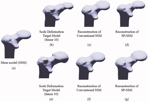
Figure 8. Two poses of DRR images were used to evaluate the scale deformation model. The femoral head of the proximal part is artificially enlarged by 20% in the deformation model.

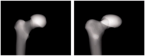
Table 2. Reconstruction error of the conventional method and the proposed method with two different sizes in the head scale deformation model. The head part was reduced by 20% or increased by 20% in the model.

	Conventional SSM (mm)	Proposed SPSSM (mm)	Conventional SSM (mm)	Proposed SPSSM (mm)
Femur number	Scale factor 0.8		Scale factor 1.2
1	3.60	3.04	3.55	3.45
2	5.72	4.24	3.59	2.80
3	4.39	2.96	3.33	2.55
4	7.09	2.78	6.09	2.68
5	4.59	3.65	4.01	3.28
6	3.93	3.59	3.23	2.35
7	4.28	3.82	3.21	2.90
8	5.36	5.21	4.44	4.04
9	5.44	2.88	6.62	2.99
10	3.46	3.17	3.36	2.61
11	4.07	3.91	4.87	3.66
12	4.48	3.50	5.06	3.95
Average	4.70	3.56	4.28	3.10

Discussion

We investigated the reason why the SPSSM performed better than the SSM. The size of the femoral head in the SPSSM case was enlarged or foreshortened by 20% under the influence of the eigenvector corresponding to the largest eigenvalue, arranged as one of the columns of the eigenvector matrix ${\mathbf{\Phi }}_{{\mathbf{p}}_{\mathit{k}}},$ which was found to be related to the effect of making the 3D model larger or smaller. However, the eigenvector in $\mathbf{\Phi }$ tended to enlarge or foreshorten the overall shape, which resulted in the failure of the conventional SSM to reduce the reconstruction error. For example, if only one part of a shape is made larger to reduce the error in the conventional SSM, the remaining parts also become larger, which in turn tends to an increase the error. Another reason for the smaller reconstruction error in SPSSMs was that segmented shapes are independently aligned in the reconstruction process, which is one of the reasons why the SPSSM has less reconstruction error than the SSM in the case of angle deformation of femoral anteversion. As an alternative to SPSSM, we can consider a stack or collection of independent SSMs in which an independent SSM is built on each segmented shape. This method seems to be promising at the first sight. However, segmenting specific parts from all the training shapes is a prerequisite for building independent SSMs, but reliable segmentation of part of a shape is challenging, especially when the shape under consideration is not composed of distinct parts, as is the case with the femur. When we try to develop a stack of SSMs, we can expect another problem. The 3D shape models should be broken down into multiple parts by automatic or manual segmentation to build individual SSMs. The segmentation procedure should be repeated for all the training datasets. The 3D vertices are in correspondence with each other in all the training datasets. When imperfect segmentation occurs, a vertex is assigned to one training dataset, while its corresponding vertex is assigned to another dataset. The unmatched vertices must be removed to build an SSM for each segment. When these partial SSMs are assembled into a final 3D model, the remaining vertices must be reconnected for a proper model because of lost vertices. The salient feature of our method is that we obtain segmented ${\mathbf{\Phi }}_{{\mathbf{p}}_{\mathit{k}}}$ by retaining the rows of $\mathbf{\Phi }$ related to landmarks without building SSMs one by one, because we partition only the final target model and group the landmarks included in each segment. So far, we have discussed the SPSSM for a single object. However, the SSM can be extended to model multiple objects. For example, one recent study [29] treated the eight small bones of the wrist, which was employed for diagnosing injuries of the wrist bones. The overall SSM was composed of several SSMs which individually represented the small bones. Each object was separated spatially from the other but pose information could be imposed on the SSMs. Similarly, a multi-object SSM was used in the reconstruction of knee anatomy [30], as the knee joins the femur to the tibia. However, we break a connected object into several parts by force and try to describe the broken parts using independent SSMs. This method corresponds to the stack of SSMs problem and inherits the same problems discussed above. We can also compare SPSSM with marginalized GPMM [21,22]. GPMM can be marginalized to the specific local region by using customized kernels which include spatially-varying kernels. The marginalized GPMM needs the design of the individual kernel functions, the combination of kernels and the adjustment of the kernel parameters to localize the region of interest and delimit its range. On the contrary, SPSSM can break down the mean model of the conventional SSM into several segments of anatomical interest by direct visual inspection and decision of the surgeon, which is simpler and faster. The concept of SPSSM can be applied to other types of SSMs without kernel functions such as SSM based on surrogate variables [19] and rSSM [20]. While GPMM is regarded as a generalized version of SSM, SPSSM can be considered the marginalized GPMM with the kernel functions.

Next, we discuss the issue of segmentation of proximal and distal femurs from X-ray images in a clinical situation. The segmentation of the proximal femur in X-ray images is regarded as a difficult problem, since the proximal femur shows low contrast in intensity distribution, overlaps the pelvic bone, and at the same time, its shape and size can differ from person to person. Even though the proximal femur segmentation is a challenging task, a series of studies on this issue has been undertaken steadily [31–34]. The authors of these studies used various techniques, such as U-net [31], an atlas-based method [32], active contours with curvature constraints [33], and an active shape model [34]. The distal part of the femur also needs to be segmented. A recent study [35] performed robust automatic segmentation to extract the distal femur and proximal tibia contours from knee X-ray images by using the spectral clustering and active shape model. The study reported accurate segmentation results for the distal femur and the tibia. The authors reported that the segmentation results were robust and accurate, and these segmentation methods seem to have been employed successfully in medical diagnosis. It can be noted that our research purpose is to propose the SPSSM under the assumption that femur segmentation can be successfully performed, leading to the successful outer boundary description of the femur used in the experiments. If a satisfactory segmentation algorithm is not available, we can resort to the manual extraction method or the semi-automatic method, since the number of X-ray images needed in the 3D reconstruction is quite limited. Actually, two X-ray images could produce a target model in our experiment.

Conclusions

In this work, we presented an SPSSM which enabled us to partition a shape into two or more segments and to find an SSM for each segment independently. The advantage of the SPSSM is that we can avoid the complicated procedure of building an SSM for each segment, adopting the procedure of dividing the shape into segments and calculating the eigenvectors using PCA for the corresponding covariance matrix. In the SPSSM, we can divide the given eigenvector matrix $\mathbf{\Phi }$ into a segment-based eigenvector ${\mathbf{\Phi }}_{{\mathbf{p}}_{\mathit{k}}}$ simply by retaining the rows of $\mathbf{\Phi }$ corresponding to the landmarks of the segment of a shape and filling the remaining rows with zeros. The SPSSM can be used for the problem of patient-specific personalization of the human femur. Two deformation cases were presented to demonstrate the validity of the SPSSM concept. The first case was concerned with the deformation of the femoral anteversion angle, and the second was concerned with the deformation of the femoral head size. In these two cases, the shape variations were quite severe, beyond the scope of the collected training femur datasets, or only part of a shape was subjected to severe distortion. In the latter case, the size of the femoral head was enlarged or foreshortened by 20%. The experimental results for the two deformation cases showed that the SPSSMs performed better than the conventional SSMs for both cases in terms of the reconstruction error.

Disclosure statement

None of the authors have potential conflicts of interest to be disclosed.

Additional information

Funding

This work was supported by the Technology Innovation Program (Grant No. 10063309) funded by the Ministry of Trade, Industry and Energy of Korea, was also supported by the Basic Science Research Program through the National Research Foundation of Korea (NRF) funded by the Ministry of Education (2020R1I1A1A01064673), and was also supported by the technology transfer and commercialization program through INNOPOLIS Foundation funded by the Ministry of Science and ICT (2021-DG-RD-0031/Fraction reduction system for precise rotational correction).

References

- Cootes TF, Taylor CJ, Cooper DH, et al. Active shape models-their training and application. Comput Vision Image Understanding. 1995;61(1):50–59.
- Reyneke CJF, Lüthi M, Burdin V, et al. Review of 2-D/3-D reconstruction using statistical shape and intensity models and X-ray image synthesis: toward a unified framework. IEEE Rev Biomed Eng. 2019;12:269–286.
- Baka N, Kaptein BL, de Bruijne M, et al. 2D-3D shape reconstruction of the distal femur from stereo X-ray imaging using statistical shape models. Med Image Anal. 2011;15(6):840–850.
- Chan CS, Edwards PJ, Hawkes DJ. Integration of ultrasound-based registration with statistical shape models for computer-assisted orthopedic surgery. Med Imag. 2003;5032:414–424.
- Fleute M, Lavallée S. Nonrigid 3-D/2-D registration of images using statistical models. In International Conference on Medical Image Computing and Computer-Assisted Intervention. Berlin, Heidelberg: Springer; 1999. p. 138–147.
- Benameur S, Mignotte M, Parent S, et al. 3D/2D registration and segmentation of scoliotic vertebrae using statistical models. Comput Med Imaging Graph. 2003;27(5):321–337.
- Zheng G, Gollmer S, Schumann S, et al. A 2D/3D correspondence building method for reconstruction of a patient-specific 3D bone surface model using point distribution models and calibrated X-ray images. Med Image Anal. 2009;13(6):883–899.
- Rajamani KT, Styner MA, Talib H, et al. Statistical deformable bone models for robust 3D surface extrapolation from sparse data. Med Image Anal. 2007;11(2):99–109.
- Sherouse GW, Novins K, Chaney EL. Computation of digitally reconstructed radiographs for use in radiotherapy treatment design. Int J Radiat Oncol Biol Phys. 1990;18(3):651–658.
- Yao J. Assessing accuracy factors in deformable 2D/3D medical image registration using a statistical pelvis model. In Proceedings Ninth IEEE International Conference on Computer Vision. IEEE; 2003. p. 1329–1334.
- Yu W, Chu C, Tannast M, et al. Fully automatic reconstruction of personalized 3D volumes of the proximal femur from 2D X-ray images. Int J Comput Assist Radiol Surg. 2016;11(9):1673–1685.
- Cerveri P, Sacco C, Olgiati G, et al. 2D/3D reconstruction of the distal femur using statistical shape models addressing personalized surgical instruments in knee arthroplasty: a feasibility analysis. Int J Med Robotics Comput Assist Surg. 2017;13(4):e1823.
- Cerveri P, Belfatto A, Manzotti A. Predicting knee joint instability using a Tibio-femoral statistical shape model. Front Bioeng Biotechnol. 2020;8:253.
- Youn K, Park MS, Lee J. Iterative approach for 3D reconstruction of the femur from un-calibrated 2D radiographic images. Med Eng Phys. 2017;50:89–95.
- Kim H, Lee K, Lee D, et al. 3D reconstruction of leg bones from x-ray images using CNN-based feature analysis. In 2019 International Conference on Information and Communication Technology Convergence (ICTC). IEEE; 2019. p. 669–672.
- Kasten Y, Doktofsky D, Kovler I. End-to-end convolutional neural network for 3D reconstruction of knee bones from bi-planar X-ray images. In International Workshop on Machine Learning for Medical Image Reconstruction. Cham: Springer, 2020. p. 123–133.
- O’Connor J, Rutherford M, Hill J, et al. Statistical shape model based 2D–3D reconstruction of the proximal femur—influence of radiographic femoral orientation on reconstruction accuracy. In Computer Methods in Biomechanics and Biomedical Engineering. Springer, Cham, 2018. p. 153–160.
- O'Connor JD, Hill JC, Beverland DE, et al. Influence of preoperative femoral orientation on radiographic measures of femoral head height in total hip replacement. Clin Biomech. 2021;81:105247.
- Blanc R, Reyes M, Seiler C, et al. Conditional variability of statistical shape models based on surrogate variables. In International Conference on Medical Image Computing and Computer-Assisted Intervention. Berlin, Heidelberg: Springer; 2009. p. 84–91.
- Zhang J, Malcolm D, Hislop-Jambrich J, et al. An anatomical region-based statistical shape model of the human femur. Comput Methods Biomech Biomed Eng Imag Vis. 2014;2(3):176–185.
- Lüthi M, Gerig T, Jud C, et al. Gaussian process morphable models. IEEE Trans Pattern Anal Mach Intell. 2018;40(8):1860–1873.
- Fouefack JR, Borotikar B, Douglas TS, et al. Dynamic multi-object gaussian process models. In International Conference on Medical Image Computing and Computer-Assisted Intervention. Cham: Springer; 2020. p. 755–764.
- Mitschke M, Navab N. Recovering the X-ray projection geometry for three-dimensional tomographic reconstruction with additional sensors: Attached camera versus external navigation system. Med Image Anal. 2003;7(1):65–78.
- Tsai RY, Lenz RK. Real time versatile robotics hand/eye calibration using 3D machine vision. In Proceedings 1988 IEEE International Conference on Robotics and Automation. IEEE; 1988. p. 554–561.
- Karmarkar N. A new polynomial-time algorithm for linear programming. In Proceedings of the Sixteenth Annual ACM Symposium on Theory of Computing. New York (NY): Association for Computing Machinery; 1984. p. 302–311.
- Pieper S, Halle M, Kikinis R. 3D Slicer. In 2004 2nd IEEE International Symposium on Biomedical Imaging: Nano to Macro (IEEE Cat No. 04EX821). IEEE; 2004. p. 632–635.
- Efron B. Estimating the error rate of a prediction rule: improvement on cross-validation. J Am Stat Assoc. 1983;78(382):316–331.
- Shefelbine SJ, Carter DR. Mechanobiological predictions of femoral anteversion in cerebral palsy. Ann Biomed Eng. 2004;32(2):297–305.
- Van de Giessen M, Foumani M, Streekstra GJ, et al. Statistical descriptions of scaphoid and lunate bone shapes. J Biomech. 2010;43(8):1463–1469.
- Baka N, Kaptein BL, Giphart JE, et al. Evaluation of automated statistical shape model based knee kinematics from biplane fluoroscopy. J Biomech. 2014;47(1):122–129.
- Lianghui F, Gang HJ, Yang J, et al. Femur segmentation in X-ray image based on improved U-Net. In IOP Conference Series: Materials Science and Engineering. IOP Publishing. 2019;533(1):012061.
- Ding F, Leow WK, Howe TS. Automatic segmentation of femur bones in anterior-posterior pelvis x-ray images. In International Conference on Computer Analysis of Images and Patterns. Springer, Berlin, Heidelberg, 2007. p. 205–212.
- Chen Y, Ee X, Leow WK, et al. Automatic extraction of femur contours from hip x-ray images. International workshop on computer vision for. Biomed Image Appl. 2005;3765:200–209.
- Pilgram R, Walch C, Kuhn V, et al. Proximal femur segmentation in conventional pelvic X ray. Med Phys. 2008;35(6):2463–2472.
- Wu J, Mahfouz MR. Robust x-ray image segmentation by spectral clustering and active shape model. J Med Imaging. 2016;3(3):034005.