Performance assessment of surgical tracking systems based on statistical process control and longitudinal QA

Abstract

A system for performance assessment and quality assurance (QA) of surgical trackers is reported based on principles of geometric accuracy and statistical process control (SPC) for routine longitudinal testing. A simple QA test phantom was designed, where the number and distribution of registration fiducials was determined drawing from analytical models for target registration error (TRE). A tracker testbed was configured with open-source software for measurement of a TRE-based accuracy metric $\epsilon$ and Jitter ($J$). Six trackers were tested: 2 electromagnetic (EM – Aurora); and 4 infrared (IR − 1 Spectra, 1 Vega, and 2 Vicra) – all NDI (Waterloo, ON). Phase I SPC analysis of Shewhart mean ($\overline{x}$) and standard deviation ($s$) determined system control limits. Phase II involved weekly QA of each system for up to 32 weeks and identified Pass, Note, Alert, and Failure action rules. The process permitted QA in <1 min. Phase I control limits were established for all trackers: EM trackers exhibited higher upper control limits than IR trackers in $\epsilon$ (EM: ${\overline{x}}_{\epsilon }\mathrm{ }\sim$2.8–3.3 mm, IR: ${\overline{x}}_{\epsilon }\mathrm{ }\sim$1.6–2.0 mm) and Jitter (EM: ${\overline{x}}_{\mathrm{jitter}} \sim$0.30–0.33 mm, IR: ${\overline{x}}_{\mathrm{jitter}}\mathrm{ }\sim$0.08–0.10 mm), and older trackers showed evidence of degradation – e.g. higher Jitter for the older Vicra (p-value < .05). Phase II longitudinal tests yielded 676 outcomes in which a total of 4 Failures were noted − 3 resolved by intervention (metal interference for EM trackers) – and 1 owing to restrictive control limits for a new system (Vega). Weekly tests also yielded 40 Notes and 16 Alerts – each spontaneously resolved in subsequent monitoring.

Keywords:

• Surgical navigation
• quality assurance
• statistical process control
• target registration error

1. Introduction

Surgical trackers are prevalent in minimally invasive surgery, including intracranial neurosurgery [1,2], spine surgery [3,4], joint reconstruction [5], and head and neck surgery [6]. However, there is a lack of standardized, streamlined quality assurance (QA) protocols to monitor tracking performance. A variety of methods for measurement of geometric accuracy have been developed for different surgical tracking systems – drawing, for example, from the American Society for Testing and Materials guidelines on measurement and reporting of tracking system accuracy under defined conditions [7]. Such testing is mostly applicable to calibration and characterization of optical/infrared (IR) tracking systems at the manufacturer’s site, as in [8]. A variety of measurement protocols have also been reported for tracker assessment in a laboratory environment for IR or electromagnetic (EM) trackers, including protocols for volumetric calibration and static or dynamic phantom measurements [9], assessment of tilt angle impact on instrument tracking accuracy [10] and commercially available tools like the Accuracy Assessment Kit (NDI, Waterloo ON) [11]. An overview of proposed validation approaches for EM tracking was described in [12], including guidelines for the design of assessment protocols.

While several approaches have been described for the assessment of tracker accuracy in the operating room (OR) [13–16], there is currently a lack of standardized procedures suitable to routine quality assurance (QA) in clinical settings. This, despite the fact that trackers are often cited as a source of uncertainty or frustration in clinical use. Common impediments include uncertainty in the accuracy of the current tracker-to-image registration, perceived geometric errors for which the cause is unclear (e.g. perturbation of the reference marker, deformation of patient anatomy, or degradation in the tracker itself), and common frustrations associated with marker occlusion, line-of-sight obstruction, or metal interference. Assured quality in the performance of the tracking system itself could mitigate some of these uncertainties, accelerate troubleshooting, improve their value in common clinical use, and avoid unnecessary workflow gaps or service calls.

An example specification of tracker test protocols was described in AAPM Task Group 147 [17], which defined protocols for the assessment of IR [18] and EM trackers [19] in radiotherapy. In the context of surgery, protocols for tracker assessment have also been described for both IR and EM tracking systems [13,14,20]. An example, an application-specific approach was described in [16] in the context of maxillofacial surgery using a purpose-built maxilla phantom. Consistent with the need to assure (and continuously improve) the quality of technologies deployed in the OR, a generalizable method that is rigorous, quantitative, free of steep manufacturing costs, and suitable to routine use in busy workflows could be of value to medical physicists, engineers, technicians and/or manufacturer field service engineers.

Statistical process control (SPC) defines a rigorous methodology for quality control that is widely adopted in manufacturing [21]. Central to SPC are concepts of upper and lower control limits (UCL and LCL, respectively) in one or more test metrics by which continuous monitoring of a system can be evaluated. Such an approach provides a basis from which to define tolerances in each test metric and action levels for pass/failure and intervention. SPC is applicable to other frequently performed, standardized processes and promises utility in healthcare and clinical QA/quality improvement as outlined by [22,23]. For example, SPC has been recognized as a potential basis for evaluating the quality of outcomes in computer-assisted orthopedic surgery [24] and cardiac surgery [25,26].

In this work, we adopt SPC as a basis for the QA of surgical trackers. A simple, low-cost QA test phantom is described based on statistical models of target registration error (TRE), and a system of hardware and software was developed that is potentially suitable to routine QA in clinical environments. The process was demonstrated with six (EM and IR) tracking systems, starting with the SPC definition of baseline UCL and LCL tolerance levels in precision and accuracy. Longitudinal QA studies spanning up to 32 weeks were analyzed in relation to control limits for each system, and action levels were identified such that the operator could quantifiably monitor quality and identify problems that warrant intervention or service.

2. Methods

2.1. Test phantom design and analysis: a principled approach

Target registration error (TRE) is a widely recognized metric of geometric accuracy in surgical tracking – rigorously established in seminal work by Fitzpatrick et al. [27] – and is the underlying quantity of one of the key figures of merit for tracker QA proposed below. TRE quantifies the expected distance between corresponding points after tracker registration (viz., between points that were not used for tracker registration). Compared to fiducial registration error (FRE), which is uncorrelated with TRE [28], this choice provides a metric that is generalizable across systems and intuitive with respect to the goal of accurate surgical navigation. Statistical analysis of point-based registration accuracy presents a considerable subject of ongoing work [27–34], with the design and analysis below based on rigid point-based registration. Drawing from $N$ points that can be unambiguously localized in the coordinate frames of both the tracker and a 3D image within which to navigate, we choose $N_r$ points as registration fiducials ($N_r=N-1$) and evaluate TRE at the remaining target position, $x.$ Assuming isotropic, homogeneous fiducial localization error (FLE), the expected value of TRE² can be expressed as a function of the number of registration fiducials and their spatial configuration with respect to the target location, $x$ [26]: (1) $$〈{\mathrm{TRE}\left(x\right)}^2〉=\frac{1}{N_r}(1+\frac{1}{3}\sum _{k=1}^3\frac{d_k^2}{f_k^2})〈{\mathrm{FLE}}^2〉$$(1) where $d_k$ denotes the distance of a target point ($x$) from the $k$^th principal axis of the fiducial configuration, and $f_k^2$ is the mean squared distance of all registration fiducials from the $k$^th principal axis of the fiducial configuration. Note that Equation (1)(1) $$〈{\mathrm{TRE}\left(x\right)}^2〉=\frac{1}{N_r}(1+\frac{1}{3}\sum _{k=1}^3\frac{d_k^2}{f_k^2})〈{\mathrm{FLE}}^2〉$$(1) is strictly valid only when FLE is zero-mean, isotropic, and identically distributed – assumptions that are not strictly observed for real tracking systems. While Equation (1)(1) $$〈{\mathrm{TRE}\left(x\right)}^2〉=\frac{1}{N_r}(1+\frac{1}{3}\sum _{k=1}^3\frac{d_k^2}{f_k^2})〈{\mathrm{FLE}}^2〉$$(1) is therefore an approximation to the performance of real trackers, it is nevertheless a useful guide to optimizing fiducial configurations. This model was used as the basis for a principled approach to the design of a QA test phantom and the analysis by which an ensemble of TRE measurements sampled from a distribution with approximately the same expectation value can be conveniently collected in routine assessment of tracking accuracy.

As detailed below, the test phantom presents a set of unambiguous points that can be freely designated as either registration fiducials (used to compute the tracker-to-image transform) or targets (used in the analysis of TRE). Following the analysis of Hamming et al. [31], which used Equation (1)(1) $$〈{\mathrm{TRE}\left(x\right)}^2〉=\frac{1}{N_r}(1+\frac{1}{3}\sum _{k=1}^3\frac{d_k^2}{f_k^2})〈{\mathrm{FLE}}^2〉$$(1) to analyze optimal fiducial configurations for image-guided head and neck surgery, we evaluated the design of a QA test phantom in terms of the magnitude and spatial dependence of expected TRE over all target locations on the phantom as a function of the number ($N_r$) and configuration ($d_k^2/f_k^2$) of registration fiducials. To efficiently generate an ensemble of TRE measurements from a single, streamlined test conducted in routine QA, we evaluated all configurations of $N_r=N-1$ registration fiducials within $N$ points in a leave-one-out (LOO) analysis. To make efficient use of the data, we drew $N$ points from $N_{\max } = 10$ available divots on the phantom and analyzed all possible configurations, ranging from less optimal (closely spaced arrangements of few fiducials, for which the expected TRE varies with position, denoted as ‘Inferior’) to more optimal (broadly distributed arrangements of many fiducials, yielding lower, more spatially uniform expected TRE, denoted as ‘Superior’). The aim of the analysis was to find the appropriate number, $N,$ for which the expected TRE is reasonably spatially uniform across LOO configurations – e.g. 10 point localizations, giving 10 permutations of $N_r$ = 9 registration fiducials from which LOO analysis yields 10 TRE measurements with approximately the same expectation value.

Equation (1)(1) $$〈{\mathrm{TRE}\left(x\right)}^2〉=\frac{1}{N_r}(1+\frac{1}{3}\sum _{k=1}^3\frac{d_k^2}{f_k^2})〈{\mathrm{FLE}}^2〉$$(1) provides a principled approach to phantom design, extended in [32] to include anisotropic, spatially inhomogeneous FLE, which we used to further validate the anticipated behavior of TRE measured as a function of the number and spatial configuration of the fiducials, taking anisotropic (but spatially homogeneous) FLE as a fit parameter. The analytical models convey intuitively that a greater number and superior configuration of registration fiducials reduce the magnitude and spatial variation in TRE, and comparison to measurements provided both validation and a useful guide to identify a point of diminishing return with respect to the goal of a streamlined QA procedure.

2.2. System for QA of surgical trackers

2.2.1. Testbed

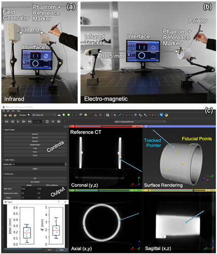
An example implementation of a system for tracker QA is shown in the benchtop setup of Figure 1. While the tracker and phantom can be freely positioned, the phantom was always repositioned at a nominal position (to within ±5 mm) with the reference marker within a few cm of the center of the measurement volume to ensure consistency across the longitudinal measurements. In principle, the same setup could be achieved on a stable, mobile cart that holds only the phantom and the computer workstation (user interface) with the tracker positioned on its normal support arm in the operating room, taking care to limit vibration of the tracker or phantom during testing.

Figure 1. Testbed for tracker QA. (a) Setup for an EM tracking system (Aurora #1), showing the field generator, phantom with reference marker, pointer, and software interface. (b) Setup for an IR tracking system (Vicra #1). (c) software interface showing coronal, axial, sagittal, and surface-rendered views of the phantom with fiducial points (yellow) overlaid after tracker-to-image registration. Also shown are the software controls and outputs of QA measurements.

2.2.2. Trackers

Measurements were performed using six tracking systems (all NDI): two electromagnetic (EM) trackers (denoted Aurora #1 and #2); two laboratory infrared (IR) trackers (denoted Vicra #1 and #2); and two clinical IR trackers (a Spectra and a Vega). The six trackers used in this work were subject to routine maintenance and/or recalibration as follows: (1) the Vicra #1 system was approximately 10 years old and gave no evidence of required recalibration since its initial deployment; (2) the Vicra #2 was approximately 6 years old and similarly gave no evidence of miscalibration; (3) the Aurora #1 was approximately 10 years old and was recalibrated once by the manufacturer (approximately six months prior to initiating this work); (4) the Aurora #2 was relatively new (2 years old) and was not recalibrated since its initial deployment; (5) the Stealth was approximately 4 years and was not recalibrated since its initial deployment; and (6) the Vega was the newest system (QA measurements for this study were started immediately after initial deployment). Overall, these systems likely experienced less routine use within a controlled research environment (weekly/monthly use within a laboratory) than systems in clinical use (daily use and subject to increased frequency of movement around the hospital). However, the extent to which they were subject to recalibration is comparable to that of clinical systems. For example, only the Aurora #2 was subject to recalibration during its lifetime when it was suspected of some degradation in performance. Similarly, the typical routine process for systems in clinical use is based on an initial check during instrument calibration with the software, and only if clear signs of failure or miscalibration are evident (presumably upon setup or use in a case) is the system recalibrated or replaced. For each system, a standard, pivot-calibrated pointer tool was used for point localization: a standard probe (NDI, part number 610065) for the Aurora systems; and a passive 4-marker probe (NDI, part number 8700340) for the Vicra, Spectra, and Vega systems. For the optical systems, the pointer tool tip was calibrated on a divot formed on a steel plate and with a conical drill bit. Calibrations were repeated 10 times, each sampling the marker for 30 s (amounting to ∼600 samples). The dispersion of the localized pointer tip was measured to be 0.84 ± 0.27 mm. The nominal sampling rate for each system was 40 Hz (Aurora), 60 Hz (Spectra and Vega), and 20 Hz (Vicra). The number of samples ($M,$ collected at the nominal sampling rate of each tracker) that was averaged to yield a single measurement point could be freely varied via the computer interface (below), and a study was conducted to identify the value of $M$ that balanced tradeoffs between a wider temporal averaging window (to reduce random electronic/quantum noise variations) and a shorter temporal averaging window (to reduce the time per measurement and avoid user-dependent instability/fatigue).

2.2.3. Test phantom

A test phantom was manufactured from a PVC cylinder (12.7 cm diameter × 9.5 cm length, with 0.5 cm wall thickness), fulfilling desirable design criteria of low cost, simplicity, ease of manufacture, rigidity, and robustness. Divot locations on the phantom’s surface were chosen drawing from the analysis in Section 2.1. A reference marker was rigidly attached to the phantom as shown in Figure 1 – a standard reference disk (NDI, part number 610066) for the EM trackers and a 4-marker dynamic reference frame (NDI, part number 8700339) for the IR trackers. Fiducial points that could be unambiguously localized with a pointer tool and in a 3D CT slice viewer were formed by the apex of conical divots (∼2 mm diameter × ∼2 mm depth) drilled in the surface of the cylinder with a 30° ‘V’ bit. For ergonomic ease of use, divots were selected in locations that could be easily reached by the operator working from one side of the cylinder, giving a total of $N$ = 10 divots within convenient reach. Note that the exact coordinates of the divots are not essential, and any distribution of fiducials leading to a reasonably narrow range of LOO TRE according to the analysis in Section 2.1 can be used to generate a QA phantom free-hand and without precise machining requirements. The reference position of each point in CT image coordinates was determined from a high-resolution CT scan (Canon Precision One CT scanner; 0.16 × 0.16 × 0.25 mm³ voxels) such that high-precision machining was not required for the phantom.

2.2.4. User interface

As illustrated in Figure 1(c), a software module for 3D Slicer [35] was developed to facilitate streamlined, routine QA tests, using the Plus toolkit [36] to interface with the tracking systems and send marker poses via the OpenIGTLink network protocol [37]. The graphical interface provides controls to connect to different trackers, collect position measurements, and save the results in a structured report. Figure 1(c) shows orthogonal slice views, a 3D surface rendering of the QA phantom, reference point locations overlaid, and the tracked pointer location (after registration). Also displayed on the interface are the position measurements and resulting figures of merit (below) resulting from a QA test (table and a boxplot).

2.3. Experimental methods

2.3.1. Metrics for tracker performance and QA

To measure the precision and accuracy of each tracker, fiducial points (divots) on the phantom were localized in the tracker and reference CT image coordinate frames. The position of each fiducial ($i\in \left\{1,\dots ,N\right\}$ fiducials) was measured by successively sampling at the fixed, default sampling rate of the tracker ($j\in \left\{1,\dots ,M\right\}$ samples), yielding positional measurements, $p_{i,j},$ in the tracker coordinate frame. The (true) reference location of each fiducial in CT image coordinates was determined (once; not with each QA test) from a mean of 10 repeats, manually localized by a single observer in a 3D orthogonal slice viewer. Two metrics were used to quantify the geometric precision and accuracy of tracker measurements:

2.3.2. Jitter ($\mathit{J}$)

For each fiducial, $i,$ the Jitter ($J_i$) was computed as the standard deviation of the distribution of position measurements $p_{i,j}.$ Jitter was evaluated as a function of the number of samples ($M$) averaged to yield a single point measurement to identify a nominal value that optimized the temporal averaging window. The median Jitter and 95% confidence interval (CI95) were determined over all point localizations, $i.$ Note that analysis of Jitter does not require distinction of ‘registration’ fiducials and ‘target’ points and simply uses all points for which there is a measurement.

2.3.3. Target registration error (TRE) based error metric $\mathit{\epsilon }$

A rigid registration transform ($T$) was computed between registration fiducials measured in the tracker coordinate frame ($p_i,$ obtained by averaging $p_{i,j}$ over $M$ samples) and corresponding reference fiducials in the CT image coordinate frame via Horn’s method using quaternions [38]. It is worth noting that the least-square solution in [38] is similarly valid (optimal) under the assumption that the FLE is zero-mean and identically distributed. While these assumptions are not strictly obeyed by real tracking systems, the method is a common choice for solving an approximate point-based registration. Future work could transcend such limitations with solutions that do not rely on such assumptions, such as the heteroscedastic error-in-variable (HEIV) solution by Matei and Meer [39]. For a given number of points ($N$) co-localized by the user, an ensemble of measurements was computed via LOO analysis (yielding $N_r=N-1$ registration markers for registration and $1$ marker, $i,$ for analysis of TRE). Target registration error for the $i$^th point (${\mathrm{TRE}}_i$) was measured as the distance between the registered point ($T{p}_i$) and its reference position. The extent to which the ensemble of TRE measurements can be considered samples from a common underlying distribution in TRE with approximately the same expectation value was investigated as a function of the number and configuration of registration fiducials. Due to the varying registration fiducial configurations, this ensemble of TRE measurements is similar, but not strictly representative of the true TRE; therefore, we subsequently refer to this LOO metric as an error, denoted $\epsilon .$ The median error, $\epsilon ,$ and CI95 were computed over all LOO configurations, $i\in \left\{1,\dots ,N\right\}.$

2.3.4. Statistical process control limits and longitudinal QA

Tracker performance was monitored according to principles of statistical process control (SPC) using 3-sigma Shewhart $\overline{x}$ and $s$ control charts, computed for both Jitter and error $\epsilon .$ Control limits were established in ‘Phase I’ measurements of the mean and standard deviation in Jitter and error $\epsilon ,$ resulting in 4 pairs of upper and lower control limits – denoted UCL and LCL, respectively, as in [40]. Specifically, the UCL and LCL for a metric mean ($\overline{x}$) is given by: (2) $$\mathrm{UCL}\left(\overline{x}\right)=\overline{\overline{x}}+3\frac{\overline{s}}{c_4\sqrt{n}}$$(2) (3) $$\mathrm{LCL}\left(\overline{x}\right)=\overline{\overline{x}}-3\frac{\overline{s}}{c_4\sqrt{n}}$$(3) where $\overline{\overline{x}}$ is the average of all observations (‘grand mean’) and $\overline{s}$ is the mean standard deviation across $m$ samples, each of size $n,$ given by $\overline{s}=\frac{1}{m}{\sum }_{i=1}^m{s}_i,$ with $s_i$ the standard deviation of the $i$^th sample. The statistic $\frac{\overline{s}}{c_4}$ is an unbiased estimator of the true sample standard deviation, where $c_4$ is given by: (4) $$c_4=\sqrt{\frac{2}{n-1}}·\frac{\left(\frac{n}{2}-1\right)!}{\left(\frac{n-1}{2}-1\right)!}$$(4) where the factorial for a non-integer argument is computed according to the definition in [40]: (5) $$\left(\frac{n}{2}\right)!=\left(\frac{n}{2}\right)\left(\frac{n}{2}-1\right)\left(\frac{n}{2}-2\right)···\left(\frac{1}{2}\right)\sqrt{\pi }$$(5)

Similarly, the UCL and LCL for the standard deviation in the metric is given by: (6) $$\mathrm{UCL}\left(s\right)=\overline{s}+3\frac{\overline{s}}{c_4}\sqrt{1-c_4^2}$$(6) (7) $$\mathrm{LCL}\left(s\right)=\overline{s}-3\frac{\overline{s}}{c_4}\sqrt{1-c_4^2}$$(7) recognizing that for metrics of Jitter and error $\epsilon ,$ the LCL may be superfluous in many cases; nevertheless, they are included in the analysis, since even abnormally low Jitter or error $\epsilon$ may signal a problem with the system. As in [40], the control limits were adjusted iteratively to reject out-of-control data points from those used to compute the control limits, with a data point defined to be out-of-control if it fell above the UCL for any of the four Shewhart charts. A minimum of $m=25$ data points was included in the control limit computation, following Shewhart’s rule of thumb to obtain ‘no less than 25 samples of size four’ [41]. Here, we obtained a larger sample size of $n=10$ (explained in more detail in 3.1).

‘Phase I’ measurements (i.e. those by which to establish control limits) for each tracking system involved 30 QA tests performed consecutively within approximately 2 h to ensure baseline consistency. Phase I analysis assumes the trackers to be operating in a normal state, which was confirmed for each tracking system in this work via previous laboratory studies of tracker accuracy. The measured mean ($\overline{x}$) in $\epsilon$ and Jitter are denoted ${\overline{x}}_{\epsilon }$ and ${\overline{x}}_{\mathrm{jitter}}$ with standard deviation ($s$) denoted $s_{\epsilon }$ and $s_{\mathrm{jitter}},$ respectively. Iteratively rejecting out-of-control points, 30 tests were sufficient to yield the minimum of 25 samples to establish control limits.

‘Phase II’ measurements involved longitudinal testing in weekly QA tests spanning up to 32 weeks for each tracker. The same measurement protocol for $\overline{x}$ and $s$ (i.e. mean and standard deviation for Jitter and error) was used as described above. In each case, the tracking system was allowed a warmup time of 5 min before a QA check. Although the temperature was not monitored, the experimental setup was located in a relatively stable environment close to standard temperature and pressure.

Table 1 summarizes a set of action rules proposed in this work for QA test outcomes – in particular, for measurements falling outside control limits. A QA check with all four test results within control limits constitutes a ‘Pass,’ of course. A single test result outside control limits triggers a ‘Note’ to the operator but does not constitute failure. Test results below LCL similarly trigger a ‘Note’ to the operator and do not constitute failure, since low Jitter or error $\epsilon$ may or may not indicate a problem; however, they may still warrant attention and judgment on the part of the operator. Two test results above UCL in the same metric category – i.e. in Jitter (${\overline{x}}_{\mathrm{jitter}}$ and $s_{\mathrm{jitter}}$) or in error $\epsilon$ (${\overline{x}}_{\epsilon }$ and $s_{\epsilon }$) – trigger an ‘Alert’ to the operator warranting further consideration – e.g. to repeat the test or monitor with vigilance in the subsequent longitudinal test. The rationale for the Alert action (cf., Fail) for two out-of-control findings in the same metric category is that the mean and standard deviation in the metric are seen to be correlated (not independent test measures) and may signal a common, underlying, spurious cause that does not warrant intervention. Two or more test results in different metric categories – i.e. in Jitter and error $\epsilon$ – constitute a ‘Fail’ and warrant action – e.g. an immediate retest, troubleshooting, intervention, and/or service.

Table 1. Summary of test outcomes associated with QA measurement results relative to established control limits.

Test result	Outcome
0 tests above UCL or below LCL	Pass
1 test above UCL	Note to operator
1 or more tests below LCL	Note to operator
2 tests above UCL in same metric category (i.e. Jitter or $\epsilon$)	Alert to operator
2 or more tests above UCL in different metric categories (i.e. Jitter and $\epsilon$)	Failure

3. Results

3.1. Analysis of QA test phantom design

Point localizations were performed for each tracking system using the test phantom of Section 2.2. Studies in which the temporal averaging window was varied showed that $M$ = 30 samples provided a reasonable tradeoff between statistical sampling and physical/user error due to vibration or fatigue. Depending on the sampling rate of the tracking system (and some latency for processing), the acquisition of $M$ = 30 successive position samples required 0.8–1.9 s, during which time the tip of the tracked instrument was statically held within the divot.

Following the rationale of Section 2.1, the extent to which the TRE is spatially uniform – and, therefore, a LOO analysis across $N$ point localizations can be expected to yield estimates of the same underlying expected value in TRE – is shown in Figures 2 and 3. In Figure 2, the range in TRE is shown across all target positions calculated in LOO analysis over all configurations of $N$ point localizations chosen from the 10 divots. For the three cases shown ($N$ = 4, 7, and 10), there are $\left(\begin{array}{c}10\\ N\end{array}\right)$ fiducial configurations, each with $N$ possible target positions in the LOO analysis. The range (and accordingly the spatial variation) in TRE decreases strongly with increasing $N.$ For the LOO corresponding to $N$ = 10 (i.e. $N_r$ = 9) the range in TRE is fairly narrow (0.8–1.4 mm); therefore, a similar expected TRE measurement is approximated for each of the ten target positions.

Figure 2. Range in TRE according to the model of Equation (1)(1) $$〈{\mathrm{TRE}\left(x\right)}^2〉=\frac{1}{N_r}(1+\frac{1}{3}\sum _{k=1}^3\frac{d_k^2}{f_k^2})〈{\mathrm{FLE}}^2〉$$(1) over all target positions in LOO analysis for all configurations of $N$ point positions ($N_r=N-1$ registration fiducials and 1 target position). Cases $N$ = 4, 7, and 10 are shown, the last giving a narrow range suggesting that all measurements are representative of a similar underlying statistical distribution in TRE. Violin plots show the range (upper and lower horizontal lines), distribution of samples (shaded envelope), and median (horizontal line). The vertical arrow signifies samples in the upper tail of the distribution.

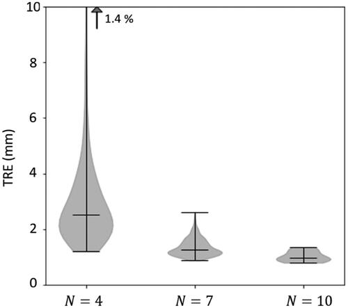
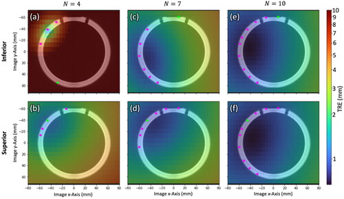
Figure 3. Spatial distribution in TRE computed by Equation (1)(1) $$〈{\mathrm{TRE}\left(x\right)}^2〉=\frac{1}{N_r}(1+\frac{1}{3}\sum _{k=1}^3\frac{d_k^2}{f_k^2})〈{\mathrm{FLE}}^2〉$$(1) over a cross section of the phantom for $N$ = 4, 7, and 10 registration fiducials for Inferior/Superior fiducial configurations. Registration fiducial/target locations (magenta/green) are projected onto the cross section. The low TRE magnitude, high degree of spatial uniformity, and similarity in TRE distributions for the $N$ = 10 case supports LOO analysis as a means to obtain 10 TRE estimates in a single QA test with 10 measurement points.

Figure 3 depicts the spatial distribution in TRE according to Equation (1)(1) $$〈{\mathrm{TRE}\left(x\right)}^2〉=\frac{1}{N_r}(1+\frac{1}{3}\sum _{k=1}^3\frac{d_k^2}{f_k^2})〈{\mathrm{FLE}}^2〉$$(1) superimposed on an axial image of the phantom for $N$ = 4, 7, and 10 point localizations for example fiducial configurations that are Inferior/Superior with respect to TRE magnitude and spatial uniformity. In each slice, the locations of registration fiducials and target positions are projected onto the axial image as magenta and green circles, respectively. The overall magnitude of TRE as well as the spatial variation decreases with an increasing number of fiducials for both configurations. For LOO analysis with $N$ = 10, the TRE distribution in Figure 3(e,f) is seen to be fairly constant throughout the cross section (also quantified in the narrow distribution range in Figure 2) and is similar between the Inferior/Superior configurations. Therefore, considering the expected range and spatial distribution in TRE for $N$ = 10, similar measurement results can be expected for all ten configurations of registration fiducials. Accordingly, the LOO analysis across $N$ = 10 point positions suggests a reasonable means to conveniently collect an ensemble of ten TRE measurements with each QA check (cf., repeating 10 times).

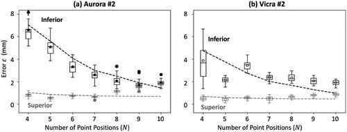
Figure 4 shows measurements of error $\epsilon$ as a function of the number of measured point positions $N$ [for the Superior (gray) and Inferior (black) configurations] from data acquired in Phase I definition of control limits. The examples shown correspond to one EM tracker (Aurora #2) and one IR tracker (Vicra #2). Note that each boxplot contains 30 samples of the error ($\epsilon$) corresponding to a single, example configuration (not an ensemble of LOO configurations). Also shown in Figure 4 are theoretical model fits according to the analysis of [32] (dashed lines) which follow the measured data reasonably well. A certain level of discrepancy is anticipated in light of the coarse assumptions on anisotropic, spatially homogeneous FLE, though agreement overall is within ∼1 mm. For example, for the superior configurations for $N$>7, we observe an increasing error ($\epsilon$) that deviates somewhat from the theoretical fit. The deviation can possibly be attributed to the fact that the $N$>7 configurations included, in particular, fiducials # 1-3, which were located at the edge of the fiducial distribution on the phantom and required the user to hold the pointer tool a bit differently than for other fiducial points – namely, pointing upwards. It is possible, therefore, that for both the Vicra and the Aurora trackers, those fiducials exhibited higher FLE than the others, such that the measurements deviated from the theoretical fit that assumed spatially homogeneous FLE. Another exception for the $N$ = 5 instance in Figure 4(b) is believed to be associated with measurements resulting in anomalously low error $\epsilon ,$ not a systematic discrepancy from theory. For both tracking systems, the results confirm the flattening trend in $\epsilon$ for $N$ = 10, with a small difference between the Inferior/Superior configurations, further justifying the LOO method as a means to conveniently collect an ensemble of measurements of error $\epsilon$ drawn from distributions with nearly equivalent expectation value. (For the N = 10 configuration, both the Superior and Inferior arrangements are within the LOO-ensemble for the single fiducial arrangement).

Figure 4. Measurements of error $\epsilon$ (from Phase I definition of control limits) as a function of the number of point positions for a single example Superior (gray) and Inferior (black) fiducial configuration. (a) Electromagnetic tracker (Aurora #2). (b) infrared tracker (Vicra #2). theoretical model fits are shown as dashed lines.

3.2. Control limits and longitudinal QA

3.2.1. Phase I: control limits

Figure 5 shows the Phase I measurements for all six tracking systems in Jitter (top row) and error $\epsilon$ (bottom row) as well as the resulting upper and lower control limits (red and blue, respectively) shown as vertical and horizontal lines. Data points iteratively rejected from the control limit computation are marked with a red circle, noting that the only rejections were due to high values in the Jitter mean and/or standard deviation; no data points were rejected due to higher-than normal error $\epsilon ,$ indicating that Jitter is within statistical control, but appears to be less stable than $\epsilon .$

Figure 5. Control limits in Jitter (top row) and error $\epsilon$ (bottom row) for the six tracking systems. Data points rejected from the analysis are marked with a red circle, leaving at least 25 measurements for the establishment of upper and lower control limits.

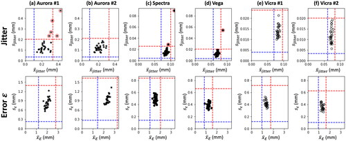
The resulting control limits for each system are summarized in Table 2. Upper control limits in mean Jitter were found to be higher for the EM trackers (${\overline{x}}_{\mathrm{jitter}}$ ∼0.30–0.33 mm) than for the IR trackers (${\overline{x}}_{\mathrm{jitter}}$ ∼0.08–0.10 mm). Similarly, control limits on Jitter standard deviation were an order of magnitude higher for EM trackers ($s_{\mathrm{jitter}}$ ∼0.20 mm) than for IR trackers ($s_{\mathrm{jitter}}$ ∼0.02–0.03 mm). Consistent with expectations, the EM trackers also exhibit slightly higher UCL in mean error $\epsilon$ (${\overline{x}}_{\epsilon }$ ∼2.8–3.3 mm) compared to the IR trackers (${\overline{x}}_{\epsilon }$ ∼1.6–2.0 mm). Interestingly, the EM trackers also exhibit higher UCL in $\epsilon$ standard deviation ($s_{\epsilon }$ ∼1.5 mm for the EM trackers, compared to ∼0.6–0.8 mm for the IR trackers). Overall, the newer and older systems performed similarly – for example, the Vicra #1 and Vicra #2 systems yielding nearly identical UCL and LCL in each metric. The newer wide baseline IR system (Vega) exhibited an improved (lower) UCL in ${\overline{x}}_{\epsilon }$ and $s_{\epsilon }$ compared to the older counterpart (Spectra) (both p-values < .05), confirming the improvement in accuracy found by [42]. Interestingly, the two Vicra systems also appeared to yield improved (lower) UCL in ${\overline{x}}_{\epsilon }$ and $s_{\epsilon }$ (both p-values < .05) compared to the (even older) Spectra system.

Table 2. Upper and lower control limits for the mean and standard deviation in Jitter and error $\epsilon$ for each tracking system.

Tracker	Metric	LCL (mm)	UCL (mm)
Aurora #1	${\overline{x}}_{\mathrm{jitter}}$	0.11	0.33
	$s_{\mathrm{jitter}}$	0.03	0.20
	${\overline{x}}_{\epsilon }$	1.21	2.79
	$s_{\epsilon }$	0.23	1.39
Aurora #2	${\overline{x}}_{\mathrm{jitter}}$	0.09	0.33
	$s_{\mathrm{jitter}}$	0.04	0.21
	${\overline{x}}_{\epsilon }$	1.44	3.28
	$s_{\epsilon }$	0.27	1.62
Spectra	${\overline{x}}_{\mathrm{jitter}}$	0.07	0.10
	$s_{\mathrm{jitter}}$	0.004	0.03
	${\overline{x}}_{\epsilon }$	1.08	2.02
	$s_{\epsilon }$	0.14	0.83
Vega	${\overline{x}}_{\mathrm{jitter}}$	0.06	0.08
	$s_{\mathrm{jitter}}$	0.003	0.02
	${\overline{x}}_{\epsilon }$	0.87	1.62
	$s_{\epsilon }$	0.11	0.66
Vicra #1	${\overline{x}}_{\mathrm{jitter}}$	0.07	0.10
	$s_{\mathrm{jitter}}$	0.004	0.02
	${\overline{x}}_{\epsilon }$	0.96	1.77
	$s_{\epsilon }$	0.12	0.71
Vicra #2	${\overline{x}}_{\mathrm{jitter}}$	0.06	0.08
	$s_{\mathrm{jitter}}$	0.003	0.02
	${\overline{x}}_{\epsilon }$	0.96	1.67
	$s_{\epsilon }$	0.10	0.63

3.2.2. Phase II: longitudinal QA measurements

Longitudinal QA tests resulting from each tracking system are summarized in Figure 6. Data points triggering either a Note, Alert, or Failure (Table 1) are marked in blue, yellow, or red, respectively. Across up to 32 weeks of QA testing of each system (676 test outcomes in total), a total of 40 Notes, 16 Alerts, and 4 Failures were reported. The somewhat forgiving set of action rules (Notes and Alerts in Table 1) is intended to keep the operator aware of potential issues without triggering unnecessary false alarms for retesting or service calls. For example, most Alerts were associated with exceeding the UCL in Jitter (${\overline{x}}_{\mathrm{jitter}}$ or $s_{\mathrm{jitter}}$), and such were typically spurious, with the system returning to normal performance the following week (e.g. spurious vibration).

Figure 6. Phase II longitudinal QA tests for each tracking system. UCL and LCL are marked by red and blue dashed lines, respectively. Interventions are marked by red arrows. Consistent with Table 1, Notes are marked by blue circles, Alerts are marked by yellow circles, and Failures are marked by red circles.

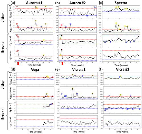
For both EM trackers, Alerts and Failures were evident in week 1 and 2. These were subsequently attributed to metal interference identified in proximity to the measurement volume, and the setup was adjusted accordingly. Specifically, the field generator was raised from ∼25 cm to ∼74 cm height above the metal testbed as shown in Figure 1. After this adjustment (interventions marked by red arrows), both systems performed within control limits.

For the Spectra system, a total of 6 Alerts were reported in Phase II longitudinal studies. This is perhaps attributable to this tracking system being significantly older than the others. This system also triggered 7 Notes, most of which were due to the mean $\epsilon$ falling below the LCL. This suggests that the initial Phase I control limits may have been too high, and the control limits should be updated or reestablished. For the Vega system, there is some evidence of drift in performance over the last 4–5 weeks of measurement, triggering two Alerts due to high Jitter and a Failure due to high Jitter and error $\epsilon$ in the last QA test. This system was acquired during the course of this study, and control limits were established on the system before it entered regular use (unlike other systems, which had been used regularly prior to this study). This perhaps introduced a bias for the Vega system toward overly narrow control limits, recognizing that 4–5 data points are insufficient to infer a trend in performance, and judgment of the operator could be exercised in vigilant monitoring in subsequent QA checks.

Both Vicra systems showed stable performance, triggering just 1–2 Alerts over 32 weeks of longitudinal testing – each due to high Jitter – and no Failures. The Vicra #2 exhibited a fairly high number of 14 Notes, most of which were due to mean $\epsilon$ falling below the LCL, again indicating that the Phase I control limits could be updated.

4. Discussion

The theoretical analysis of TRE employed in Section 2.1 provided a principled approach to phantom design by considering the number and arrangement of registration fiducials not only to understand the magnitude of expected TRE but also its spatial dependence and the extent to which a LOO analysis across various arrangements could be expected to yield the same expectation value in TRE. Due to the varying arrangements within the LOO analysis, the resulting metric is not strictly representative of TRE in an actual (clinical) navigation case, and the metric is referred to accordingly simply as error, $\epsilon .$ This metric is derived from a LOO analysis over TRE measurements according to the standard definition according to the theoretical relationship of Equation (1)(1) $$〈{\mathrm{TRE}\left(x\right)}^2〉=\frac{1}{N_r}(1+\frac{1}{3}\sum _{k=1}^3\frac{d_k^2}{f_k^2})〈{\mathrm{FLE}}^2〉$$(1) . Such analysis supported the implementation of a streamlined approach for generating an ensemble of measurements of error $\epsilon$ in routine QA checks – viz., 10 point localizations from which 10 $\epsilon$ measurements could be obtained in <1 min. The QA test phantom constructed from a PVC cylinder can be easily produced in-house and does not require high-precision machining, since point location truth definitions are achieved via a high-resolution CT scan, which is accessible in most settings where minimally invasive surgery is performed.

This work adds to a considerable body of literature on tracker performance – commonly cited as achieving TRE ∼1–2 mm for IR trackers and ∼2–3 mm for EM trackers in a laboratory setting – and extends that understanding rigorously in the context of upper and lower control limits established via SPC. In terms of both error $\epsilon$ and Jitter, the UCL and LCL suggest thresholds by which acceptance testing/clinical commissioning, routine QA, and troubleshooting can be conducted more rigorously and quantifiably.

Additional test metrics could certainly be envisioned – e.g. geometric accuracy (lack of distortion) throughout the field of measurement. The current work limited the analysis to error $\epsilon$ and Jitter (with upper and lower control limits for each) for two main reasons. First, these metrics are believed to convey different aspects of tracker performance – one spatial and the other temporal (although the two are certainly not unrelated) – and therefore yield assessment in somewhat distinct terms. As an aside, we had originally also included measurements of absolute distance accuracy between localized points (analogous to error $\epsilon$ but without image-to-world registration), and it was observed that this metric closely followed the results for $\epsilon .$ With such a close correlation to measurements of error $\epsilon ,$ it was determined that the absolute distance metric added little or no additional information and was omitted from the analysis. Second, from a practical perspective, limiting the analysis to two metrics (with four control limits) simplified assessment in a few 2D plots, consistent with the goals of simplicity and a streamlined QA check. While the registration-based metric shown in this work was intentionally designed to include hardware-related error relevant to the surgical navigation process (namely the tracker and associated registration algorithm), a dynamic, registration-free accuracy metric similar to that reported in [42] could be a valuable addition to be considered in future work, enabling assessment of tracker accuracy independent of other error sources.

Comparing the control limits established in Phase I among different versions of the same tracker model (i.e. Aurora #1 and #2 or Vicra #1 and #2) similar performance was observed, but statistically significant differences (p < .05, Welch’s t-test) were evident; therefore, to avoid false alarms, best practice is likely to establish control limits for each tracking system individually, rather than apply a single set across a broad class of trackers. Two important considerations for such methodology to gain broad utilization are: (1) the test metrics pertinent to routine testing must be agreed upon and standardized; and (2) it would be helpful for manufacturers to include performance specification in terms of those test metrics for purposes of acceptance testing and commissioning by the user.

There are a variety of means by which Phase I control limits could be established. The most expedient – as done in this work – is to perform at least 25 consecutive tests immediately prior to commissioning the system for clinical use. The resulting limits are then compared to manufacturer specification for purposes of basic acceptance and constitute the thresholds by which subsequent Phase II tests will be assessed. Potential limitations in this approach include: measurements performed by a single operator could reflect a user-specific bias that does not translate to a more diverse group of users performing Phase II tests; and Phase I measurements conducted in a short interval (e.g. 2 h in this work) may be subject to environmental bias at the time of the tests – e.g. temperature or building vibration. Such factors could bias control limits toward either higher or lower values.

Alternatively, the system could be commissioned based on a single acceptance test in comparison to manufacturer specification and subsequently monitored on a routine schedule (for at least 25 tests) to establish Phase I control limits. While potentially mitigating the factors mentioned above for a single Phase I test session, this approach has the clear disadvantage that a single test for acceptance lacks statistical power and may bias the initial acceptance outcome. Moreover, it suggests an extended period of use (e.g. 25 test intervals) during which routine checks are not compared to a control limit – i.e. there is no basis by which to Fail – and errors may go undetected. Alternatively, following the establishment of control limits in a single session, one could consider evolving the control limits after deployment by pooling with Phase II measurements. Clearly, doing so requires careful consideration and invites time-dependent biases of its own; for example, if control limits are updated too frequently, they will fail to detect drift in tracker performance.

The Phase II longitudinal data demonstrate the utility of SPC to monitor tracker performance via QA tests performed with a particular frequency. Among the 676 test outcomes resulting from 6 tracking systems in this work tested in up to 32 weeks, there were a total of 40 Notes, 16 Alerts, and 4 Failures. The Notes and Alerts were cautionary and seemed to be associated with spurious factors that resolved by the subsequent test, and the Failures appeared to be associated with real factors of the test setup. The process therefore succeeded in detecting ‘assignable variations,’ and variations due to ‘common causes’ did not trigger false alarms, supporting the somewhat forgiving action rules for Notes, Alerts, and Failures defined in Table 1. It is worth noting, of course, that offline QA as described here does not guarantee a low level of geometric error within a particular case (which can be confounded by suboptimal patient registration, anatomical deformation, etc.), but it does provide assurance that the tracker itself is operating within control limits.

The proposed process is pertinent to the development of routine QA protocol in clinical environments. With a streamlined protocol requiring a few minutes for physical setup and warmup and <1 min for the actual measurement, the system enables rigorous, quantitative assessment against baseline control limits and facilitates immediate verification of tracker performance by showing the measured $\epsilon$ and jitter distributions at a glance. While the methodology for establishing UCL and LCL is well defined in SPC, identifying the frequency with which tests should be performed is less well defined and is subject of future work. In the studies reported above, tests were performed weekly in order to test and demonstrate the principles of SPC in the context of surgical trackers in a relatively short total time (32 weeks); however, there is no evidence in this work that such a high frequency would be warranted in routine clinical QA. No errors were detected that necessitated a service call by the manufacturer, and while a firm answer on the frequency of such tests deserves more consideration, these studies suggest that a monthly or quarterly interval could be sufficient to give reasonable assurance of system performance.

The testbed could in principle be translated to a mobile cart, and the measurement process is suitable to being carried out by a medical physicist, engineer, technician, or vendor representative/field service engineer. Conducting such tests in-house, however, requires that the tracking systems permit interfacing via open protocols. For the NDI systems in laboratory use, this was straightforward in the current study. Although not included in the longitudinal results shown above, we successfully integrated the system with a commercially available clinical tracking system (StealthStation™ S7, Medtronic, Minneapolis MN) via the (‘StealthLink’) communication protocol made available by the manufacturer (The StealthStation system was not included in results shown above for reasons of brevity and because the system suffered a failure unrelated to the QA tests early in the work). Access to tracker communication protocols in an ‘engineering mode’ would support routine QA by hospital engineers/physicists/technicians, which in turn could mitigate some of the uncertainties in the quality of surgical trackers, improve the quality of systems in the field, and reduce unnecessary troubleshooting or service calls for issues unrelated to the tracker. Moreover, the methods described above could augment the toolkit of field service engineers in commissioning and routine preventative maintenance.

5. Conclusions

A process for QA of surgical trackers was realized based on a simple phantom designed according to a principled approach in the analysis of TRE, control limits established via SPC, and longitudinal continuity testing against established control limits with a set of action rules in the event of test results that are outside control. The test phantom is low-cost and easily manufactured, requiring a high-resolution CT scan for the definition of true point locations. The principles of SPC translated to the context of surgical trackers provide a valuable framework by which to assess tracker performance in acceptance testing/commissioning as well as routine QA. The approach was demonstrated in longitudinal studies across 6 tracking systems in up to 32 weeks of regular QA checks, showing the ability to detect assignable variations without raising false alarms. The system is potentially suitable to routine clinical QA by a medical physicist or engineer (provided communication protocols to the tracking system) and/or to field service engineers for regular preventative maintenance or troubleshooting.

Acknowledgments

The authors thank Dr. Chuck Montague (Biomedical Engineering, Johns Hopkins University) and Dr. Don Wardell (Operations and Information Systems, University of Utah) for a useful discussion of statistical process control.

Disclosure statement

The authors have no conflicts of interest related to this work. This research was supported in part by an academic-industry partnership with Medtronic (Minneapolis MN, USA) and the John C. Malone Professorship from the Whiting School of Engineering, Johns Hopkins University (Baltimore MD, USA). Data is available from the authors on reasonable request.

References

- Germano IM, Queenan JV. Clinical experience with intracranial brain needle biopsy using frameless surgical navigation. Comput Aid Surg. 1998;3(1):33–39. doi: 10.3109/10929089809148126.
- Omay SB, Barnett GH. Surgical navigation for meningioma surgery. J Neurooncol. 2010;99(3):357–364. doi: 10.1007/s11060-010-0359-6.
- Sembrano JN, Yson SC, Theismann JJ. Computer navigation in minimally invasive spine surgery. Curr Rev Musculoskelet Med. 2019;12(4):415–424. doi: 10.1007/s12178-019-09577-z.
- Virk S, Qureshi S. Navigation in minimally invasive spine surgery. J Spine Surg. 2019;5(Suppl 1):S25–S30. doi: 10.21037/jss.2019.04.23.
- Broers H, Jansing N. How precise is navigation for minimally invasive surgery? Int Orthop. 2007;31(Suppl 1):S39–S42. doi: 10.1007/s00264-007-0431-9.
- Siessegger M, Mischkowski RA, Schneider BT, et al. Image guided surgical navigation for removal of foreign bodies in the head and neck. J Craniomaxillofac Surg. 2001;29(6):321–325. doi: 10.1054/jcms.2001.0254.
- Standard ASTM. F2554-10 standard practice for measurement of positional accuracy of computer assisted surgical systems. West Conshohocken (PA): ASTM Int; 2010.
- Wiles AD, Thompson DG, Frantz DD. Accuracy assessment and interpretation for optical tracking systems. Medical Imaging 2004: Visualization, Image-Guided Procedures, and Display vol. 5367; 2004. p. 421. doi: 10.1117/12.536128.
- Frantz DD, Wiles AD, Leis SE, et al. Accuracy assessment protocols for electromagnetic tracking systems. Phys Med Biol. 2003;48(14):2241–2251. doi: 10.1088/0031-9155/48/14/314.
- Banivaheb N. Comparing measured and theoretical target registration: error of an optical tracking system. Master's Thesis, York University; 2015. http://hdl.handle.net/10315/30053
- Frantz DD, Kirsch SR, Wiles AD. Specifying 3D tracking system accuracy one manufacturer’s views. In: Proceedings of Bildverarbeitung für die medizin 2004. Berlin: Springer; 2004. p. 234–238.
- Franz AM, Haidegger T, Birkfellner W, et al. Electromagnetic tracking in medicine -A review of technology, validation, and applications. IEEE Trans Med Imaging. 2014;33(8):1702–1725. doi: 10.1109/TMI.2014.2321777.
- Teatini A, Perez de Frutos J, Lango T, et al. Assessment and comparison of target registration accuracy in surgical instrument tracking technologies. Annu Int Conf IEEE Eng Med Biol Soc. 2018;2018:1845–1848. doi: 10.1109/EMBC.2018.8512671.
- Koivukangas T, Katisko JPA, Koivukangas JP. Technical accuracy of optical and the electromagnetic tracking systems. Springerplus. 2013;2(1):90. doi: 10.1186/2193-1801-2-90.
- Wilson E, Yaniv Z, Zhang H, et al. A hardware and software protocol for the evaluation of electromagnetic tracker accuracy in the clinical environment: a multi-center study. Medical Imaging 2007: Visualization and Image-Guided Procedures, vol. 6509, 2007. p. 65092T. doi: 10.1117/12.712701.
- Seeberger R, Kane G, Hoffmann J, et al. Accuracy assessment for navigated maxillo-facial surgery using an electromagnetic tracking device. J Craniomaxillofac Surg. 2012;40(2):156–161. doi: 10.1016/j.jcms.2011.03.003.
- Willoughby T, Lehmann J, Bencomo JA, et al. Quality assurance for nonradiographic radiotherapy localization and positioning systems: report of task group 147. Med Phys. 2012;39(4):1728–1747. doi: 10.1118/1.3681967.
- Fattori G, Hrbacek J, Regele H, et al. Commissioning and quality assurance of a novel solution for respiratory-gated PBS proton therapy based on optical tracking of surface markers. Z Med Phys. 2022;32(1):52–62. doi: 10.1016/j.zemedi.2020.07.001.
- Santanam L, Noel C, Willoughby TR, et al. Quality assurance for clinical implementation of an electromagnetic tracking system. Med Phys. 2009;36(8):3477–3486. doi: 10.1118/1.3158812.
- Eppenga R, Kuhlmann K, Ruers T, et al. Accuracy assessment of wireless transponder tracking in the operating room environment. Int J Comput Assist Radiol Surg. 2018;13(12):1937–1948. doi: 10.1007/s11548-018-1838-z.
- Shewhart WA. Economic quality control of manufactured product. Bell Syst Tech J. 1930;9(2):364–389. doi: 10.1002/j.1538-7305.1930.tb00373.x.
- Benneyan JC, Lloyd RC, Plsek PE. Statistical process control as a tool for research and healthcare improvement. Qual Saf Health Care. 2003;12(6):458–464. doi: 10.1136/qhc.12.6.458.
- Mohammed MA, Cheng KK, Rouse A, et al. Bristol, shipman, and clinical governance: Shewhart’s forgotten lessons. Lancet. 2001;357(9254):463–467. doi: 10.1016/S0140-6736(00)04019-8.
- Stiehl JB, Bach J, Heck DA. Validation and metrology in CAOS. In: Stiehl JB, Konermann WH, Haaker RG, DiGioia AM, editors. Navigation and MIS in orthopedic surgery. Berlin, Heidelberg: Springer; 2007. p. 68–78. doi: 10.1007/978-3-540-36691-1_9.
- Noyez L. Control charts, Cusum techniques and funnel plots. A review of methods for monitoring performance in healthcare. Interact Cardiovasc Thorac Surg. 2009;9(3):494–499. doi: 10.1510/icvts.2009.204768.
- Shahian DM, Williamson WA, Svensson LG, et al. Applications of statistical quality control to cardiac surgery. Ann Thorac Surg. 1996;62(5):1351–1359. doi: 10.1016/0003-4975(96)00796-5.
- Fitzpatrick JM, West JB. The distribution of target registration error in rigid-body point-based registration. IEEE Trans Med Imaging. 2001;20(9):917–927. doi: 10.1109/42.952729.
- Fitzpatrick JM. Fiducial registration error and target registration error are uncorrelated. Proceedings of SPIE – The International Society for Optical Engineering, vol. 7261; 2009. p. 726102. doi: 10.1117/12.813601.
- Fitzpatrick JM, West JB, Maurer CRJ. Predicting error in rigid-body point-based registration. IEEE Trans Med Imaging. 1998;17(5):694–702. doi: 10.1109/42.736021.
- Heiselman JS, Miga MI. Strain energy decay predicts elastic registration accuracy from intraoperative data constraints. IEEE Trans Med Imaging. 2021;40(4):1290–1302. doi: 10.1109/TMI.2021.3052523.
- Hamming NM, Daly MJ, Irish JC, et al. Effect of fiducial configuration on target registration error in intraoperative cone-beam CT guidance of head and neck surgery. in 2008 30th Annual International Conference of the IEEE Engineering in Medicine and Biology Society; 2008. p. 3643–3648. doi: 10.1109/IEMBS.2008.4649997.
- Danilchenko A, Fitzpatrick JM. General approach to first-order error prediction in rigid point registration. IEEE Trans Med Imaging. 2011;30(3):679–693. doi: 10.1109/TMI.2010.2091513.
- Ma B, Ellis RE. Analytic expressions for fiducial and surface target registration error. Med Image Comput Comput Assist Interv. 2006;9(Pt 2):637–644. doi: 10.1007/11866763_78.
- Wiles AD, Likholyot A, Frantz DD, et al. A statistical model for Point-Based target registration error with anisotropic fiducial localizer error. IEEE Trans Med Imaging. 2008;27(3):378–390. doi: 10.1109/TMI.2007.908124.
- Fedorov A, Beichel R, Kalpathy-Cramer J, et al. 3D slicer as an image computing platform for the quantitative imaging network. Magn Reson Imaging. 2012;30(9):1323–1341. doi: 10.1016/j.mri.2012.05.001.
- Lasso A, Heffter T, Rankin A, et al. Plus: open-source toolkit for ultrasound-guided intervention systems. IEEE Trans Biomed Eng. 2014;61(10):2527–2537. doi: 10.1109/TBME.2014.2322864.
- Tokuda J, Fischer GS, Papademetris X, et al. OpenIGTLink: an open network protocol for image-guided therapy environment. Int J Med Robot. 2009;5(4):423–434. doi: 10.1002/rcs.274.
- Horn BKP. Closed-form solution of absolute orientation using unit quaternions. J Opt Soc Am A. 1987;4(4):629. doi: 10.1364/JOSAA.4.000629.
- Matei B, Meer P. Optimal rigid motion estimation and performance evaluation with bootstrap. Proceedings 1999 IEEE Computer Society Conference on Computer Vision and Pattern Recognition (Cat. No PR00149), vol. 1, IEEE; 1999. p. 339–345. doi: 10.1109/CVPR.1999.786961.
- Heckert N, Filliben J, Croarkin C, et al. Handbook 151: NIST/SEMATECH e-Handbook of statistical methods. Gaithersburg (MD): National Institute of Standards and Technology; 2002. (NIST Interagency/Internal Report (NISTIR)).
- Shewhart WA. Statistical method from the viewpoint of quality control. New York (NY): Dover Publications Inc.; 1937.
- Fattori G, Lomax AJ, Weber DC, et al. Technical assessment of the NDI polaris vega optical tracking system. Radiat Oncol. 2021;16(1):87. doi: 10.1186/s13014-021-01804-7.