Public transportation network scan for rapid surveillance

Abstract

As people move around using public transportation networks such as train and airplanes, it is expected that emerging infectious diseases will spread on the network. The scan statistics approach has been frequently applied to identify high-risk locations, and the results are widely used for making a clinical decision in a timely manner. However, they are not optimally designed for modeling the spread and might not effectively work in the emergency situation where computational time is essentially important. We propose a new scan statistics approach for the public transportation network, called PTNS (Public Transportation Network Scan). PTNS utilizes the available network structure to construct potential candidates of clusters, and thus it can work well especially in situations where public transportation is the main medium of the infection spread. Further, it is designed for rapid surveillance. Lastly, PTNS is generalized to detect space-time clusters by customizing the iteration for potential clusters creation. Using the simulation data generated with a real railway network, we showed that, PTNS outperformed the conventional methods, including Circular- and Flex-scan approaches, in terms of the detection performance, while the computational time is feasible.

Keywords:

• Scan statistics
• Spatio-Temporal analysis
• rapid surveillance
• public Transportation
• covid-19

1. Introduction

1.1. Previous studies and settings

Detecting high-risk geographical areas, say hotspots, of emerging infectious diseases such as COVID-19 is an important task that is expected to provide the estimates accurately and rapidly. To address it, the scan statistics approach has been frequently applied to rapidly identify the hotspots in the area of interest, and the results are widely used for making a clinical decision on medical resource allocations, prioritization, and interventions in a timely manner. In addition, the scan statistics approach has been applied not only in the field of infectious diseases but also in medical imaging, parasitology, forestry cancer epidemiology, and astronomy [1–9].

Consider a network structure with vertices and edges $G=(V,E)$, and counts $c_i$ for each vertex $s_i(\in V)$, scan statistic approach tries to detect the subset $S\subset V$, where the number or rate of interest is larger than other subsets in V. To detect the subset S with a significantly higher number or rate of interest, scan statistic approach takes following three steps. (1) construct candidate potential clusters, which are denoted by $Z_j(j=1,\dots ,M)$, and sets of $s_i$, for a given region, network, and area, (2) calculate summary (likelihood-based) statistics $D(Z_j)$, and then (3) identify the most likely cluster (MLC) that has the highest $D(Z_j)$.

For example, if we consider a train network, $s_i$ represents each station. That is, $s_1,s_2,\dots ,s_m$ represent Shinjuku, Yoyogi, and Tokyo stations, and so on, respectively. Further, $Z_j$ represents the set of stations $\{s_i\}$. The fact that $Z_j$ is a hotspot means that the stations which belong to $Z_j$ have higher infection rate than the other stations.

Various types of summary statistics in Step (2) have been proposed [10–13]. For example, Neil et al. proposed Bayesian version of summary statistics [14]. Further, Gangon and Clayton proposed weighted likelihood-based summary statistics [15].

Scan statistics approach counts the number of events $c_i$ observed in a fixed area $s_i\in S(i=1,\dots ,m)$, where S is the whole area of interest. There are three main steps:

1.2. How to construct potential clusters of scan statistics and space-time scan statistics for rapid surveillance

Here, we explain how to construct candidate potential clusters $\{Z_j{\}}_{j=1}^M$. Ideally, all possible clusters should be constructed as potential clusters: $M=2^m$ combinations should be constructed. However, it is difficult in practice because M increases exponentially as m increases, and the computational complexity becomes enormous.

To tackle it, various methods for potential cluster construction were proposed. To make potential clusters within a feasible time, these methods restrict the shape of potential clusters to certain types. Naus [16], and Loader [17] proposed a rectangle-shaped potential cluster. Also, Openshaw et al. [18], Besag and Newwell [19], and Kulldorff et al. [10] proposed a circular-shaped potential cluster, and the radius of the cluster varies. In a similar way, Christiansen et al. [20] and Kulldorff et al. [21] proposed an elliptic potential cluster. Due to the restriction on the shape, the computational time for the calculation remains reasonable. In these methods, a method proposed by Kulldorff is the most famous and widely used [10]. Software called SatScan (https://www.satscan.org/) is frequently used in various practical studies such as Azage et al. [22], Coleman et al. [23], and Sherman et al. [24].

As pointed out by Tango and Takahashi [25], although the above-mentioned methods, which construct the restricted shape of potential clusters, are useful and widely used in practice, Christiansen et al. [20], and so on, there exist the clusters whose shapes are irregular, and the existing methods cannot cover such irregularly shaped clusters.

To address it, Tango and Takahashi  proposed methods that can construct non-circle-shaped and flexible type potential clusters [25]. The details can be found elsewhere [12, 13, 25–30]. These methods are known to work well, especially when the number of potential clusters is small, and thus the computational time remains reasonable range. However, as prior studies pointed out [30–32], these methods become unfeasible due to the long computational time as the number of potential clusters goes large. In addition, in the field of computer science, there are similar attempts that use external information such as GraphScan approach [33, 34] to restrict the search space for the potential clusters.

These methods construct potential clusters from a spatial perspective, but several methods that try to extend the potential cluster from a space-time perspective have also been proposed [35, 36].

1.3. Cluster detection on public transportation network

In today's cities, there are many means of transportation, such as cars, trains, planes, and buses, and they make their unique network structure. As people move around on the network, it is expected that infection will spread on the network. In the public transportation networks, airborne, droplet, and contact infections are likely to occur. Thus, infectious diseases which are likely to be transmitted by airborne, droplet, or contact are likely to spread on the networks.

Although existing methods could theoretically be applied to the network data, they are not optimally designed for modeling the spread of infection on the network and might not effectively work on detecting clusters along with the network within the limited computational time. Circular-shaped approach might not be suitable for the detection of long consecutive clusters: i.e. when many infected persons move on a long train line, and thus the cluster takes a linearly expanded shape along with the line, Circular approach can not capture it because of its non-circular shape. In addition, although flexible type approaches can construct the arbitrary shape of potential clusters, and thus they can contain any clusters along with the network as the subset, the computational burden is heavy, and it is too slow to be used in rapid surveillance. To capture the real-time spread of infection, we need to develop a new method to construct potential clusters suitable for detecting long consecutive clusters along with a network of interest in a timely manner. Note that we assume $s_i$ is each node, which represents a station, bus stop, or car park, on a given network instead of a geographical area in the conventional scan statistics.

1.4. Contribution

To address the above issues, we propose a new scan statistics approach for the public transportation network, called PTNS (Public transportation network scan), for rapid surveillance of infectious diseases. This paper's contribution is four-fold.

1. Computational burden of our method is small compared with conventional scan methods. The number of iterations is linear in the number of nodes in the networks (Proposition 2.2).

2. Our method can detect long hotspots which are difficult to detect in the conventional methods.

3. Our method can be generalized to detect both space and space-time hotspots.

4. For the long hotspot detection, the result shows that our method outperforms the conventional methods in terms of accuracy, sensitivity, and positive predicted value.

The remainder of the article is organized as follows. In Section 2, we review the basic idea of the scan statistics approach and introduce our new scan-based method to detect high-risk clusters along with an available network structure, and then it is extended to detect space-time clusters. To demonstrate that the proposed method outperforms the conventional approaches in terms of accuracy, sensitivity, and the positive predicted values, the results using the simulation data generated with a real railway network in Japan are presented in Section 3. Finally, Section 3 contains a discussion and our conclusion.

2. Methods

Here, we describe the proposed method. First, we briefly explain the basic idea of scan statistics for count data. We follow the notations used in [37]. Let $\mathcal{G}$ be a network (also called as a graph) which consists of m nodes. $s_i(i=1,\dots ,m)$ denotes a node on the network, e.g. railway station, bus stop and car park. G is the set of $s_i$, i.e. $G:=\{s_1,\dots ,s_m\}$. $b_i$ and $c_i$ are the expected number of infected people and the observed number of infected people on the node $s_i$ for $i=1,\dots ,m$, respectively. Generally, $b_i$ is assumed to be given or calculated from the past observed data, as follows: $b_i=n_i\frac{\sum _{i=1}^m{c}_{i,past}}{\sum _{i=1}^m{n}_i},$ where $n_i$ represents the number of residents around $s_i$, the number of users of $s_i$, and so on. You can tailor $n_i$ to your problem. Then, $Z_j(j=1,\dots ,M)$ denote potential clusters, which consist of multiple nodes, e.g. $Z_j:=\{s_1,s_2,s_3\}$. The aim of scan statistics is to compare potential clusters and identify the specified $Z_j$ which has the significantly higher risk under the hypothesis testing.

2.1. Scan statistic for count data

Here we explain the specified examples of the scan statistic used in the hypothesis testing. We assume that $c_i$ follows the Poisson distribution with the mean parameter $q{b}_i$ as follows: (1) $c_i\sim \text{Po}(q{b}_i),$(1) where $\text{Po}(a)$ indicates the Poisson distribution with the mean parameter a, q represents the infection rate. Under the null hypothesis $H_0$, we assume that $c_i$ are generated by $\text{Po}(q_{all}{b}_i)$ for all $s_i\in G$, where $q_{all}$ takes the same constant rate for all $s_i\in G$. Under the alternative hypothesis $H_1(Z_j)$, we assume that $c_i$ are generated by $\text{Po}(q_{in}{b}_i)$ for all $s_i\in Z_j$ and $c_k$ are generated by $\text{Po}(q_{out}{b}_k)$ for all $s_k\in G-Z_j$, where $q_{in}$ and $q_{out}$ are some constants and $q_{in}>q_{out}$. In the above settings, the following test statistic is known [10]: (2) $\begin{array}{rl}D\left(Z_j\right):& ={\left(\frac{C_{in}}{B_{in}}\right)}^{C_{in}}{\left(\frac{C_{all}-C_{in}}{B_{all}-B_{in}}\right)}^{C_{all}-C_{in}},\\ & \text{if}\frac{C_{in}}{B_{in}}>\frac{C_{all}-C_{in}}{B_{all}-B_{in}},\end{array}$(2) and $D(Z_j):=1$ otherwise, where $C_{in}=\sum _{s_i\in Z_j}{c}_i$, $B_{in}=\sum _{s_i\in Z_j}{b}_i$, $C_{all}=\sum _{s_i\in G}{c}_i$ and $B_{all}=\sum _{s_i\in G}{b}_i$. When $C_{all}=B_{all}$, the condition $\frac{C_{in}}{B_{in}}>\frac{C_{all}-C_{in}}{B_{all}-B_{in}}$ can be reduced to $C_{in}>B_{in}$ [31]. The above scan statistic focuses on both potential clusters and the outside of them. On the other hand, Neil et al. (2005) focuses on the only potential clusters in the following sense [37]: Under the null hypothesis $H_0$, we assume that $c_i$ are generated by $\text{Po}(b_i)$ for all $s_i\in G$. Under the alternative hypothesis $H_1(Z_j)$, we assume that $c_i$ are generated by $\text{Po}(q{b}_i)$ for all $s_i\in Z_j$ and $c_k$ are generated by $\text{Po}(b_k)$ for all $s_k\in G-Z_j$, where q is some constant and q>1. The test statistic $D(Z_j)$ is represented as follows: (3) $D(Z_j):={\left(\frac{C_{in}}{B_{in}}\right)}^{C_{in}}\exp (B_{in}-C_{in}),\text{if}{B}_{in}>C_{in},$(3) and $D(Z_j):=1$ otherwise. Here we provide the following relation for these scan statistics.

Proposition 2.1

Under $C_{all}=B_{all}$ and $C_{all}\to \mathrm{\infty }$, the Equations (2(2) $\begin{array}{rl}D\left(Z_j\right):& ={\left(\frac{C_{in}}{B_{in}}\right)}^{C_{in}}{\left(\frac{C_{all}-C_{in}}{B_{all}-B_{in}}\right)}^{C_{all}-C_{in}},\\ & \text{if}\frac{C_{in}}{B_{in}}>\frac{C_{all}-C_{in}}{B_{all}-B_{in}},\end{array}$(2) ) and (3(3) $D(Z_j):={\left(\frac{C_{in}}{B_{in}}\right)}^{C_{in}}\exp (B_{in}-C_{in}),\text{if}{B}_{in}>C_{in},$(3) ) are equivalent.

Proof.

From the Equation (2(2) $\begin{array}{rl}D\left(Z_j\right):& ={\left(\frac{C_{in}}{B_{in}}\right)}^{C_{in}}{\left(\frac{C_{all}-C_{in}}{B_{all}-B_{in}}\right)}^{C_{all}-C_{in}},\\ & \text{if}\frac{C_{in}}{B_{in}}>\frac{C_{all}-C_{in}}{B_{all}-B_{in}},\end{array}$(2) ), $\begin{array}{rl}D\left(Z_j\right)& ={\left(\frac{C_{in}}{B_{in}}\right)}^{C_{in}}{\left(\frac{C_{all}-C_{in}}{B_{all}-B_{in}}\right)}^{C_{all}-C_{in}}\\ & ={\left(\frac{C_{in}}{B_{in}}\right)}^{C_{in}}{(1+\frac{B_{in}-C_{in}}{B_{all}-B_{in}})}^{C_{all}-C_{in}}\\ & ={\left(\frac{C_{in}}{B_{in}}\right)}^{C_{in}}{\left\{{(1+\frac{B_{in}-C_{in}}{C_{all}-B_{in}})}^{\frac{C_{all}-C_{in}}{B_{in}-C_{in}}}\right\}}^{B_{in}-C_{in}}.\end{array}$ Then, we have $\to {\left(\frac{C_{in}}{B_{in}}\right)}^{C_{in}}\exp (B_{in}-C_{in})\text{ as }{C}_{all}\to \mathrm{\infty }.\text{■}$

With these statistics, we can detect the clusters whose count of interest is higher than expected. For all M potential clusters, we calculate $\{D(Z_j){\}}_{j=1}^M$. Then, MLC with the highest $D(Z_j)$ is selected. We confine our interest to the efficient construction of set of potential clusters $\{Z_j{\}}_{j=1}^M$ for rapid surveillance of infectious disease.

2.2. Proposed algorithm: PTNS

Let $|S|$, K, and $A_i$ be the size of set S, maximum size of a potential cluster, and the set of nodes that is adjacent to $s_i$ on a given network or in a given geographical area. Define the distance between two nodes $s_i$, and $s_j$ as $d(s_i,s_j)$.

There are several possible distance measures: for example, Euclidean distance between two geographical locations or network-connectivity-based distance such as passenger volume between two stations. Further, travel time between two stations can be used as the distance measure. Then, we construct the list of potential clusters $\{Z_{ik}{\}}_{i=1,\dots ,m,k=1,\dots ,K}$ as the following Algorithm 1.

Lastly, the constructed $Z_{ik}$ with the highest $D(Z_{ik})$ defined in Equation (2(2) $\begin{array}{rl}D\left(Z_j\right):& ={\left(\frac{C_{in}}{B_{in}}\right)}^{C_{in}}{\left(\frac{C_{all}-C_{in}}{B_{all}-B_{in}}\right)}^{C_{all}-C_{in}},\\ & \text{if}\frac{C_{in}}{B_{in}}>\frac{C_{all}-C_{in}}{B_{all}-B_{in}},\end{array}$(2) ) is selected as the MLC. The set $\{Z_{ik}{\}}_{i=1\dots ,m,k=1,\dots ,K}$ is equivalent with $Z_j$ in the above. The following proposition guarantees the computational efficiency or equivalence of PTNS, which is measured by the number of internal iterations, and compared with other conventional scan statistics approach. Algorithm ?? directly induces the following proposition:

Proposition 2.2

PTNS requires $\mathcal{O}(mK)$ iterations to construct size of (at most) K-nodes potential cluster centered at each m-node. Thus, the number of iterations is linear in the size of potential cluster K. The same order can be applied to Circular-scan statistics developed by [10]: i.e. Circular-scan algorithm requires $\mathcal{O}(mK)$ iterations. On the other hand, Flex-scan algorithm developed by [25] requires $\mathcal{O}(m{K}^2)$ iterations to construct size of K-nodes potential cluster centered at each m-node. Thus, The number of iterations is exponential in the size of potential cluster K.

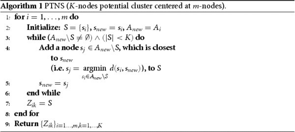
It is worth noting that, although PTNS has the same iteration order $\mathcal{O}(mK)$ to that of the Circular-scan, PTNS can capture any clusters that are along with the network structure and thus be able to identify clusters that have a longer diameter of a given network $\mathcal{G}$, as shown in the simulation data analysis section. Figure 1 illustrates the examples of characteristic clusters detected by each algorithm. It shows that Circular-scan approach tends to detect a circular-shaped cluster centered with one station, and Flex-scan tends to have a smaller diameter of the cluster on the network because the clusters tend to become compact in one place with many short branches on the network. In contrast, PTNS tends to detect a cluster with a larger diameter on the network because it expands the set of potential clusters along with the network structure. Therefore, PTNS can work well in situations where the railway is the major media of the infection spreads.

Figure 1. Examples of detected clusters by each algorithm: Proposed (Top), Circular-scan (Bottom left), and Flex-scan (Bottom right).

2.3. Extension of PTNS to space-time potential clusters

We have explained how to construct spatial potential clusters for spatial scanning, but the idea of the cluster can be easily extended from a space-time perspective [38–41]. Here we assume only the nodal attribute (i.e. $c_i$) is time-varying and other network structure is time-invariant.

Let T, and $Z_{j,t}(j=1,\dots ,M,t=1,\dots ,T)$ be the number of time points, and the jth potential cluster at time t, respectively. Assume that the set of nodes included in $Z_{j,t}$ is fixed same over time. We construct a list of space-time potential clusters, which is denoted as $\{Z_{j,t_s:t_e}{\}}_{j=1\dots ,M,t_s=1,\dots T,t_e=1,\dots ,T,t_s\le t_e}$, between time $t_s$, and $t_e$ ($t_s\le t_e$) as follows.

In addition, we can apply this method to other algorithms. By using this algorithm, we make space-time potential clusters for other space potential cluster generating algorithms in the following simulation study.

3. Simulation data analysis result

3.1. Settings

In this section, we examine the performance of PTNS by using a simulation data generated with the Japan railway (JR) network in Tokyo. Figure 2 shows the train station network. The black line and gray circle indicate train lines, and an 800-m ball centered at each station.

Figure 2. JR network in Tokyo: black line is JR railway line, and gray circle is 800-m ball centered at each station.

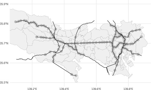
JR network in Tokyo includes 142 train stations and 22 lines. We simulate one true space-time cluster, each of which is a set of stations, and check the performance of our, and conventional algorithms, including Circular-, and Flex-scan approaches, for identifying the true cluster. When constructing potential clusters by PTNS, Circular and Flex-scan, we need to decide what kind of the distance measure we use. In this study, we use geographical Euclidean distance. Of course, as we mentioned in the previous section, we can use other distances such as passenger volume and travel time between two stations. We denote the ith station at time t by $s_{i,t}(i=1,\dots ,142,t=1,\dots ,T)$.

The procedure to prepare for the true clusters is as follows:

1. Select n as the size of a true cluster H

2. Select a line randomly

3. Select the sequential n-stations on the line randomly and set the n-station as a true cluster H

4. Select the number of time points T from $\{1,2,3,4,5\}$ randomly

5. Select $t_s$ as the start-time of the true cluster from $\{1,\dots ,T\}$ randomly

6. Select $t_e$ as the start-time of the true cluster from $\{t_s\dots ,T\}$ randomly

7. Extend H to $H_{t_s:t_e}$, which represents a true time-space cluster

8. For each station at time of t, $s_{i,t}\in H_{t_s:t_e}$, generate the number of patient $c_{i,t}\sim \text{Po(200)}$

9. For each station at time of t, $s_{i,t}\notin H_{t_s:t_e}$, generate the number of patient $c_{i,t}\sim \text{Po(100)}$

$Po(a)$ is a Poisson distribution with the mean parameter a. We assume that there is only one true cluster in the JR network, and its size varies from 5 to 20 ($n=5,\dots ,20$). We perform Monte Carlo simulations 100 times for each n.

3.2. Evaluation metrics

For the MLCs detected by each method in each setting, we calculate the accuracy, sensitivity, and positive predicted value (PPV) to compare the performance. The evaluation metrics are defined as follows.

Let H, and M represent the set of stations in one true cluster, and in one MLC, respectively.

We define accuracy as $\text{Accuracy}=\{\begin{array}{ll}1& (H=M)\\ 0& (\text{otherwise}),\end{array}$ which measures the exact detection power of each algorithm. An algorithm with high accuracy can detect the true cluster more accurately than an algorithm with low accuracy.

Sensitivity is defined as the proportion of stations detected correctly among the stations in the true cluster: $\text{Sensitivity}=|M\cap H|/|H|.$ PPV is defined as $\text{PPV}=|M\cap H|/|M|.$ PPV is the proportion of stations detected correctly among the stations in the MLC. These metrics are often used in the studies of scan statistics [42, 43].

3.3. Computational efficiency of PTNS

The number of potential clusters that were created in each algorithm is shown in Table 1. For each K, each algorithm provides potential clusters. Note that as the number of potential clusters increases, the computational time becomes longer.

Table 1. Number of potential clusters created in each algorithm.

K	PTNS	Circular	Flex
1	142	142	142
2	240	240	227
3	344	366	365
4	449	488	505
5	559	602	673
6	661	721	935
7	766	841	1288
8	870	960	1846
9	966	1086	2627
10	1064	1206	4083
11	1156	1331	6169
12	1240	1452	9714
13	1326	1574	16443
14	1407	1695	26744
15	1483	1818	40987
16	1554	1940	68974
17	1621	2063	107915
18	1683	2185	183180
19	1742	2302	302465
20	1798	2420	513992

The number of potential clusters generated by the proposed method is about 1.35, and 285.87 times smaller than that of Circular-, and Flex-scan algorithms, resulting in a shorter computational time. In our experimental environment (CPU: Intel Xeon (R) Gold 6242, 2.8GHz, Memory: 384 GB), each computation for creating potential clusters is taken 0.91, 0.10, and 31.55 seconds for the proposed, Circular-, and Flex-scan methods, respectively, in the case of K = 20. As mentioned in Proposition 2.2, the number of potential clusters generated by the proposed, and Circular-scan methods increases in a linear order. On the other hand, the number of potential clusters generated by the Flex-scan methods increases in an exponential order.

Note that, in addition to the creation of potential clusters, the calculation of $D(Z_j)$ is required, whose iterations also take as many times as the iteration for the creation of potential clusters. It means that the total computational time of the whole procedure, including the creation of potential clusters in Algorithm 1 or 2, and the calculation of $D(Z_j)$, in Circular- and Flex-scan should be 1.35 × (the number of potential clusters in Circular-scan), and 285.87 × (the number of potential clusters in Flex-scan) times longer than that of PTNS.

The result implies that the proposed method can provide the estimated high-risk area without spending much time, which is a similar computational burden with Circular-scan.

3.4. Performance results

Figure 3 shows the results of 100 simulations for each true cluster size n $(n=5,\dots ,20)$. In terms of accuracy, when n is small, Flex-scan is superior to the proposed method, and Circular-scan (n = 5: Proposed = 0.47, Flex-scan = 0.84, Circular = 0.17). In contrast, as n increases, the proposed method outperforms Flex-scan, and the accuracy of Flex-scan converges to almost 0, which is same with that of Circular scan ($n=20$: Proposed = 0.09, Flex-scan = 0.00, Circular = 0.00). A similar trend is observed in the sensitivity: as n increases, the proposed method outperforms the conventional methods: when n = 5: Proposed = 0.85 (0.20), Flex-scan = 0.96 (0.09), and Circular = 0.79 (0.22), and when n = 20: Proposed = 0.81 (0.13), Flex-scan = 0.63 (0.10), and Circular = 0.57 (0.14). In terms of PPV, when n is small, Flex-scan provides slightly better performance than the proposed method, and Circular-scan (n = 5: Proposed = 0.91 (0.19), Flex-scan = 0.99 (0.04), and Circular = 0.84 (0.20)). However, the PPV of the proposed method is equivalently high with that of Flex-scan, especially when n>10 (n = 20: Proposed = 0.98 (0.03), Flex-scan = 1.00 (0.00), and Circular = 0.81 (0.16)).

Figure 3. Simulation results: Accuracy, Sensitivity, Positive predicted value (PPV) and calculation time (second) of proposed (PTNS), Circular-, and Flex-scan approaches.

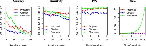
These results imply that given the large true cluster, the proposed method PTNS can work better than the conventional methods, especially in terms of accuracy, and sensitivity.

4. Conclusion and discussion

In this study, we proposed a new method of scan statistics, PTNS, with the information of the public transportation network to construct potential clusters that stretch along with the network structure. PTNS is tailored for the rapid surveillance of emerging infectious diseases such as COVID-19. It means that the goal of this study is to propose a faster but accurate algorithm for detecting high-risk areas of infectious diseases under the emergency situation where the computational time the method takes to provide results is essentially important, and our method is expected to be used in a special situation where high-risk areas should be rapidly identified and shut down immediately. Given this goal, we showed that PTNS outperforms the conventional methods, including Circular- (fast but not accurate), and Flex-scan (slow but accurate), by using the Using the simulation data generated with the real railway network: PTNS succeeds in identifying true high-risk clusters with better performance than the other methods while the computational burden still remains in the preferable range. Especially, the results show that PTNS is superior to Circular- and Flex-scan approaches in terms of the accuracy, and sensitivity of detecting true clusters when the true cluster is large.

As the limitations of PTNS, it is noteworthy that it highly depends on the available network structure. For example, the iterations in PTNS will stop if the node is on a loop. Another limitation is that PTNS does not contain a mechanism to return to the original node, and it tends to grow only in one direction along with the network, thus they may not work well in networks that show complex branching. In the fields of change detection in network structure or surveillance, there are various studies related to the identification of the hot-spots. These studies include applications such as social network detection [44], financial market analysis [45], network traffic monitoring [46], and detection of natural disasters [47]. These studies try to detect the changes in summary information on network by using the field-specific information. When considering the epidemic of infectious diseases, human mobility is a crucial factor for understanding disease transmission [48, 49]. That is, the utilization of the information on passenger volume or travel time between two stations mentioned in Section 2 is important. In addition, PTNS utilizes only the information on the simple distance metric between each node. However, network structure contains more additional information, which we can utilize as $d()$ in Algorithm ?? instead of the simple distance metric [50]: e.g. cumulative edge weight, centrality, hierarchical structure, and similarity between sub-networks. For example, the idea of the shortest path between two nodes might work well here because the human and the associated infection are assumed to move to their destination node along with the shortest path to save their mobility time [51]. In addition, when we consider a public transportation system in a real world, it might be a mixture of several networks such as buses, trains, and airplanes. To model such a mixture network, one idea is to consider the union of available networks (i.e. $G_1\cup G_2\cup \cdots \cup G_M=G_{union}$, where $G_m(m=1,\dots ,M)$ is a one public transportation network structure.) and define an appropriate $d()$ on $G_{union}$.

Disclosure statement

Mr Kentaro Matsuura reports personal fees from Chugai Pharmaceutical Co., Ltd., outside the submitted work.

Data availability statement

In this study, we do not use real data.

Additional information

Funding

This work was partially supported by KAKENHI Grant-in-Aid for Young Scientists (21K17292), KAKENHI Grant-in-Aid for Research Activity Start-up (19K24340), Daiwa Securities Health Foundation, a grant from the Ministry of Education, Culture, Sports, Science and Technology of Japan (21H03203), and Precursory Research for Embryonic Science and Technology from the Japan Science and Technology Agency (JPMJPR21RC).

Notes on contributors

Yuta Tanoue

Dr Yuta Tanoue is an Assistant Professor in the Institute for Business and Finance, Waseda University, Tokyo, Japan. His research interests include data science for finance and management.

Daisuke Yoneoka

Dr Daisuke Yoneoka is a Chief of the Epidemiology and Statistics unit at Infectious Disease Surveillance Center, National Institute of Infectious Diseases. His research interests include statistics and its applications of related fields.

Takayuki Kawashima

Dr Takayuki Kawashima is an Assistant Professor in the Department of Mathematical and Computing Science at Tokyo Institute of Technology, Tokyo, Japan. His research interests include mathematical statistics and its applications of related fields.

Shinya Uryu

Mr Shinya Uryu is an Engineer working with National Institute for Environmental Studies (NIES). He is passionate about data science, management and statistics. His favorite open-source language is R.

Shuhei Nomura

Dr Shuhei Nomura is an Associate Professor working in the Department of Health Policy and Management, School of Medicine, Keio University, Tokyo, Japan; and an Assistant Professor of the Department of Global Health Policy, Graduate School of Medicine, The University of Tokyo, Tokyo Japan. His major research interests include global burden of disease, global health policy, biostatistics, and epidemiology.

Akifumi Eguchi

Dr Akifumi Eguchi is an Assistant Professor in the Department of Sustainable Health Science, Center for Preventive Medical Sciences, Chiba University, Chiba, Japan. His research interests include statistics and its applications of related fields as well as environmental impact assessment.

Koji Makiyama

Mr Koji Makiyama is an Engineer working with HOXO-M Inc., Tokyo, Japan. His research interest includes data science and biostatistics.

Kentaro Matsuura

Mr Kentaro Matsuura is an Engineer working with Chugai Pharmaceutical Co., Ltd. Tokyo, Japan. He is also a student of Department of Management Science, Graduate School of Engineering, Tokyo University of Science, Tokyo, Japan. His research interest includes data science and biostatistics.

References

- Kulldorff M, Feuer EJ, Miller BA, et al. Breast cancer clusters in the northeast united states: a geographic analysis. Am J Epidemiol. 1997;146(2):161–170.
- Fukuda Y, Umezaki M, Nakamura K, et al. Variations in societal characteristics of spatial disease clusters: examples of colon, lung and breast cancer in Japan. Int J Health Geogr. 2005;4(1):16.
- Malleson N, Andresen MA. Spatio-temporal crime hotspots and the ambient population. Crime Sci. 2015;4(1):1–8.
- Dahly D, Gilthorpe M. P1-16 a latent class analysis of socioeconomic status and obesity in young adults from Cebu, Philippines. J Epidemiol Community Health. 2011;65(Suppl 1):A71–A71.
- Tuia D, Ratle F, Lasaponara R, et al. Scan statistics analysis of forest fire clusters. Commun Nonlinear Sci Numer Simul. 2008;13(8):1689–1694.
- Yoshida M, Naya Y, Miyashita Y. Anatomical organization of forward fiber projections from area te to perirhinal neurons representing visual long-term memory in monkeys. Proc Natl Acad Sci. 2003;100(7):4257–4262.
- Enemark HL, Ahrens P, Juel CD, et al. Molecular characterization of Danish Cryptosporidium parvum isolates. Parasitology. 2002;125(4):331.
- Coulston JW, Riitters KH. Geographic analysis of forest health indicators using spatial scan statistics. Environ Manage. 2003;31(6):764–773.
- de La Fuente Marcos R, de La Fuente Marcos C. From star complexes to the field: open cluster families. Astrophys J. 2008;672(1):342–351.
- Kulldorff M. A spatial scan statistic. Commun Stat-Theor Meth. 1997;26(6):1481–1496.
- Neill DB, Cooper GF. A multivariate Bayesian scan statistic for early event detection and characterization. Mach Learn. 2010;79(3):261–282.
- Shiode S. Street-level spatial scan statistic and STAC for analysing street crime concentrations. Trans GIS. 2011;15(3):365–383.
- Shiode S, Shiode N. A network-based scan statistic for detecting the exact location and extent of hotspots along urban streets. Comput Environ Urban Syst. 2020;83:101500.
- Neill D, Moore A, Cooper G. A Bayesian spatial scan statistic. Adv Neural Inf Process Syst. 2005;18:1003–1010.
- Gangnon RE, Clayton MK. A weighted average likelihood ratio test for spatial clustering of disease. Stat Med. 2001;20(19):2977–2987.
- Naus JL. Clustering of random points in two dimensions. Biometrika. 1965;52(1–2):263–266.
- Loader CR. Large-deviation approximations to the distribution of scan statistics. Adv Appl Probab. 1991;23(4):751–771.
- Openshaw S, Charlton M, Wymer C, et al. A mark 1 geographical analysis machine for the automated analysis of point data sets. Int J Geogr Inf Syst. 1987;1(4):335–358.
- Besag J, Newell J. The detection of clusters in rare diseases. J R Stat Soc: Ser A (Stat Soc). 1991;154(1):143–155.
- Christiansen LE, Andersen JS, Wegener HC, et al. Spatial scan statistics using elliptic windows. J Agric Biol Environ Stat. 2006;11(4):411–424.
- Kulldorff M, Huang L, Pickle L, et al. An elliptic spatial scan statistic. Stat Med. 2006;25(22):3929–3943.
- Azage M, Kumie A, Worku A, et al. Childhood diarrhea exhibits spatiotemporal variation in northwest Ethiopia: a satscan spatial statistical analysis. PLoS ONE. 2015;10(12):e0144690.
- Coleman M, Coleman M, Mabuza AM, et al. Using the satscan method to detect local malaria clusters for guiding malaria control programmes. Malar J. 2009;8(1):68.
- Sherman RL, Henry KA, Tannenbaum SL, et al. Peer reviewed: applying spatial analysis tools in public health: an example using satscan to detect geographic targets for colorectal cancer screening interventions. Prev Chronic Dis. 2014;11:
- Tango T, Takahashi K. A flexibly shaped spatial scan statistic for detecting clusters. Int J Health Geogr. 2005;4(1):421.
- Patil GP, Taillie C. Upper level set scan statistic for detecting arbitrarily shaped hotspots. Environ Ecol Stat. 2004;11(2):183–197.
- Duczmal L, Assuncao R. A simulated annealing strategy for the detection of arbitrarily shaped spatial clusters. Comput Stat Data Anal. 2004;45(2):269–286.
- Shiode S, Shiode N, Block R, et al. Space-time characteristics of micro-scale crime occurrences: an application of a network-based space-time search window technique for crime incidents in Chicago. Int J Geogr Inf Sci. 2015;29(5):697–719.
- Quick M, Law J. Exploring hotspots of drug offences in Toronto: a comparison of four local spatial cluster detection methods. Can J Criminol Crim Justice. 2013;55(2):215–238.
- Torabi M, Rosychuk RJ. An examination of five spatial disease clustering methodologies for the identification of childhood cancer clusters in Alberta, Canada. Spat Spatiotemporal Epidemiol. 2011;2(4):321–330.
- Tango T, Takahashi K. A flexible spatial scan statistic with a restricted likelihood ratio for detecting disease clusters. Stat Med. 2012;31(30):4207–4218.
- Rashidi P, Wang T, Skidmore A, et al. Spatial and spatiotemporal clustering methods for detecting elephant poaching hotspots. Ecol Modell. 2015;297:180–186.
- Cadena J, Chen F, Vullikanti A. Near-optimal and practical algorithms for graph scan statistics with connectivity constraints. ACM Trans Knowl Discov Data (TKDD). 2019;13(2):1–33.
- Speakman S, McFowland III E, Neill DB. Scalable detection of anomalous patterns with connectivity constraints. J Comput Graph Stat. 2015;24(4):1014–1033.
- Ishioka F, Kurihara K, Suito H, et al. Detection of hotspots for three-dimensional spatial data and its application to environmental pollution data. J Environ Sci Sustain Soc. 2007;1:15–24.
- Mennis J, Guo D. Spatial data mining and geographic knowledge discovery – an introduction. Comput Environ Urban Syst. 2009;33(6):403–408.
- Neill DB, Moore AW, Sabhnani M, et al. Detection of emerging space-time clusters. Proceedings of the eleventh ACM SIGKDD international conference on Knowledge discovery in data mining; 2005. p. 218–227.
- Rao H, Shi X, Zhang X. Using the Kulldorff's scan statistical analysis to detect spatio-temporal clusters of tuberculosis in Qinghai province, China, 2009–2016. BMC Infect Dis. 2017;17(1):1–11.
- Butt UM, Letchmunan S, Hassan FH, et al. Spatio-temporal crime hotspot detection and prediction: a systematic literature review. IEEE Access. 2020;8:166553–166574.
- Tang J-H, Tseng T-J, Chan T-C. Detecting spatio-temporal hotspots of scarlet fever in Taiwan with spatio-temporal Gi* statistic. PLoS ONE. 2019;14(4):e0215434.
- Agarwal S, Yadav L, Thakur MK. Circular and cylindrical hotspots detection for spatial and spatio-temporal data. 2019 Twelfth International Conference on Contemporary Computing (IC3); IEEE; 2019. p. 1–5.
- Jung I, Kulldorff M, Klassen AC. A spatial scan statistic for ordinal data. Stat Med. 2007;26(7):1594–1607.
- Jung I, Ali M. Spatial scan statistics for matched case-control data. PLoS ONE. 2019;14(8):e0221225.
- Yu R, He X, Liu Y. Glad: group anomaly detection in social media analysis. ACM Trans Knowl Discov Data (TKDD). 2015;10(2):1–22.
- Durante D, Dunson DB. Bayesian dynamic financial networks with time-varying predictors. Stat Probab Lett. 2014;93:19–26.
- Sun J, Tao D, Faloutsos C. Beyond streams and graphs: dynamic tensor analysis. Proceedings of the 12th ACM SIGKDD international conference on Knowledge discovery and data mining; 2006. p. 374–383.
- Cheng H, Tan P-N, Potter C, et al. A robust graph-based algorithm for detection and characterization of anomalies in noisy multivariate time series. 2008 IEEE International Conference on Data Mining Workshops; IEEE; 2008. p. 349–358.
- Nomura S, Tanoue Y, Yoneoka D, Gilmour S, Kawashima T, Eguchi A, Miyata H. Mobility Patterns in Different Age Groups in Japan during the COVID-19 Pandemic: a Small Area Time Series Analysis through March 2021. Journal of Urban Health. 2021;98(5):635–641. https://doi.org/10.1007/s11524-021-00566-7.
- Nomura S, Yoneoka D, Tanoue Y, et al. Time to reconsider diverse ways of working in Japan to promote social distancing measures against the covid-19. J Urban Health. 2020;97(4):457–460.
- Brandes U. Network analysis: methodological foundations. Vol. 3418, New York: Springer Science & Business Media; 2005.
- Kolaczyk ED, Csárdi G. Statistical analysis of network data with R. Vol. 65, New York: Springer; 2014.