A long short-term memory model for forecasting the surgical case volumes at a hospital

Abstract

Surgical procedures are the primary source of expenditures and revenues for hospitals. Accurate forecasts of the volume of surgical cases enable hospitals to efficiently deliver high-quality care to patients. We propose an algorithm to forecast the expected volume of surgical procedures using multivariate time-series data. This algorithm uses feature engineering techniques to determine factors that affect the volume of surgical cases, such as the number of available providers, federal holidays, weather conditions, etc. These features are incorporated in a long short-term memory (LSTM) network to predict the number of surgical procedures in the upcoming week. The hyperparameters of this model are tuned via grid search and Bayesian optimization techniques. We develop and verify the model using historical data of daily case volume from 2014 to 2020 at an academic hospital in North America. The proposed model is validated using data from 2021. The results show that the proposed model can make accurate predictions six weeks in advance, and the average $R^2$ = 0.855, RMSE = 2.017, MAE = 1.104. These results demonstrate the benefits of incorporating additional features to improve the model’s predictive power for time series forecasting.

Keywords:

• Clustering
• forecasting surgical case volume
• feature engineering
• long short-term memory model
• machine learning algorithm

1. Introduction

Surgical procedures are the main source of expenditures and revenues for hospitals. A study by Best et al. (2020) showed that, in 2017, there were over 14.6 million elective inpatient and outpatient surgical procedures in the USA. The total annual cost of these procedures was $129.9 billion, and the corresponding annual net income was $47.1 to $61.6 billion. These expenditures are due to the cost of labor (surgeon, anesthesia provider, nurses), cost of operating room (OR), cost of surgical implants, etc. A study by Muñoz et al. (2010) showed an expected 59.5% increase in surgical expenditures in 2025 as compared to 2005. This increase is mainly due to expanding and aging populations (Lim & Mobasher, 2012). Other factors that impact these costs are inefficiencies in the scheduling of OR cases and OR staff. These inefficiencies lead to overtime use or idle time of these critical resources (Bam et al., 2017). The overreaching goal of this research is to reduce the cost of healthcare by developing tools that provide high quality forecasts of the expected volume of surgical procedures. These forecasts lead to better planning, thus, better use of resources needed to operate the ORs.

Hospitals use forecasting models to determine the expected volume of surgical cases in the next week or the next month. These forecasts are used to determine the OR schedule, nurse schedule, order surgical implants, medication, and supplies, plan for capacity extensions, etc. (Jones et al., 2002; Zinouri et al., 2018). Accurate forecasts enable hospitals to efficiently use critical resources while delivering high-quality care to patients. Improving the efficiency of critical resources leads to savings and reduces waste, which contribute to reducing the cost of healthcare. The accuracy of forecasting models is impacted by the variability in the volume of surgical cases. This variability is due to patient, and provider scheduling preferences, cancelations, emergencies, and add-on cases (Zinouri et al., 2018). Additionally, the volume of surgical procedures is seasonal since patients prefer to schedule surgery during certain times of the year, such as holidays, or at the end of the fiscal year of their insurance plans (Boyle et al., 2012). These realities make forecasting challenging, and forecasting errors often raise doubt about the value of using forecasting models in hospitals. Nevertheless, historical data has often been used to predict the volume of surgical cases (Tiwari et al., 2014; Zinouri et al., 2018).

Most of the literature provides examples of time-series forecasting models being used to determine the expected number of emergency patients, surgical volume, patient flow, and demand for resources (Aravazhi, 2021). The most popular methods used in healthcare analytics are the auto-regressive integrated moving average (ARIMA), seasonal ARIMA (SARIMA), vector auto-regressive (VAR), VAR moving average (VARMA), etc. (Box et al., 2015; Ekström et al., 2015; Lütkepohl, 2006). The underlying assumption of these models is that the time series is a linear function of past values and random errors. However, ARIMA models fail to capture the nonlinear patterns often observed in time series from real-life problems, providing accurate forecasts only for a short period of time, etc. (Zhang, 2003). The aforementioned limitations have motivated researchers to develop and use machine learning (ML) and deep learning models for time series forecasting. Some of the algorithms used include support vector machine (SVM), artificial neural networks (ANN), convolutional neural networks (CNN), recurrent neural networks (RNN), long short-term memory network (LSTM), multilayer perceptron (MLP), etc. (Ahmed et al., 2010; Cui et al., 2016; Kaushik et al., 2020; Lipton et al., 2015; Pham et al., 2016; Widiasari et al., 2017; Zhao et al., 2017). Although these approaches show improvement over the statistical time-series techniques, their performance varies depending on the applications, especially in health care.

A number of companies provide support for time-series forecasting for different business applications. For example, Facebook’s Prophet is an open-source forecasting tool that is simple, easy to interpret, and highly configurable (Taylor & Letham, 2017). However, it shares some limitations with the additive models and works primarily on a univariate time series.

The proposed work is motivated by inefficiencies observed in the forecasting of the surgical case volume at a major hospital in North America. We propose a tool to forecast the surgical case volume. The development of this tool is assisted by data preprocessing and exploration, feature engineering, model development, and model deployment and monitoring. The proposed forecasting model is developed using data about the daily volume of surgical cases from 2014 to 2019. The model is validated using data from 2021. Next, we provide details of the models developed (Section 2), experimental results (Section 3), and conclusions (Section 4).

2. Methods

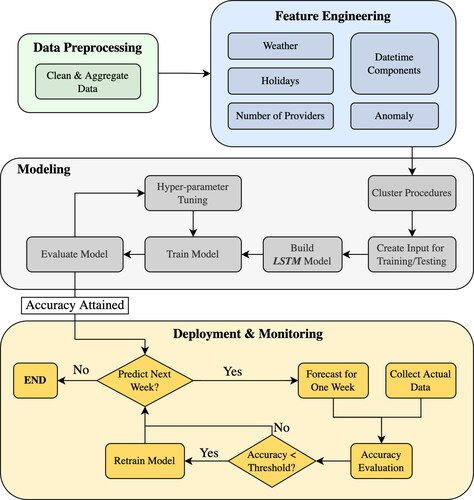
This study focuses on developing a tool to forecast the volume of weekly surgical cases at an academic hospital in North America. Figure 1 presents the framework of the proposed study. It includes a data analysis step, feature engineering, model development and training, and forecasting. Next, we provide details about each step.

Figure 1. Modeling framework.

2.1. Data preprocessing and analysis

We obtained data for the period May 2014 to September 2021 from the Arkansas Clinical Data Repository (UAMS, 2021). The dataset keeps a record of the day of the surgery, service type, a description of the surgical procedure, patient information, location of the operating room (OR), and surgeon and staff names. The dataset contains a total of 133,468 records (cases). These records represent a total of 1,865 different procedures, which belong to 27 different service types. An identification number is associated with each procedure (referred to as proc_id). To protect sensitive information of the data, we randomly generate a unique synthetic number (SID) per procedure.

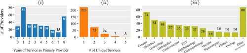
Figure 2 summarizes the data related to primary providers (doctors) and the services provided. There is a total of 330 doctors in this hospital. We notice that many doctors performed surgeries for one year or less (see Figure 2(i)). This is mainly because the majority of the doctors in the database are students who complete their one-year long medical residency in this (academic) hospital. Most of the doctors perform surgeries that belong to a single service type (see Figure 2(ii)). The most popular services are general, obstetrics, and gynecology (see Figure 2(iii)).

Figure 2. Data associated with the primary providers and services provided. Distribution of the (i) primary providers based on years of service; (ii) unique services per provider; (iii) number of surgical procedures by service during May 2014 to September 2021 (data of 2020 is excluded).

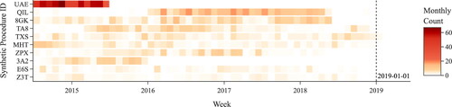
A number of procedures were discontinued after December 2018. Figure 3 maps the frequency of observations over time for ten procedures that were discontinued. Hence, we did not consider these procedures in our model development.

Figure 3. Heat map of ten procedures that were not scheduled after December 2018.

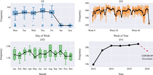
Based on Figure 4(iv), the volume of surgical cases increased from 2014 to 2019. There was a significant decrease in the volume of cases during 2020 because of the COVID-19 pandemic. Since 2020 was not a typical year, we decided not to consider the corresponding data in our analysis. We observe a significant difference in the volume of cases scheduled during the week and weekend (Figure 4(i)). We also noticed that there is no statistically significant difference in the volume of cases among months of the year (Figure 4(iii)) and among weekdays (Figure 4(i)). In addition, the volume of cases is generally lower for the weeks during which there is a major holiday. For example, the volume of cases is lowest during the week of July 4th (week 23) and the week between Christmas and New Year (week 53) (Figure 4(ii)).

Figure 4. Distribution of the volume of surgical cases based on (i) day of the week, (ii) week of year, (iii) month of the year, and (iv) total number per year.

2.2. Feature engineering

We initially developed a univariate time series to forecast the volume of surgical cases per week. This time series contained a count of the number of surgical cases per week and per surgical procedure. The outcomes of this time series forecasting were not encouraging. Thus, to improve the accuracy of our forecasting model, we engineered a few features by manipulating the raw data (Zheng & Casari, 2018). This process transformed our univariate into a multivariate time series. This transformation enhanced the accuracy of our prediction model. Other studies use feature engineering to improve the quality of predictions for healthcare applications. A study by Vollmer et al. (2021) uses feature engineering to capture the impact of school holidays on demand at an emergency department (ED). Similarly, a study by McCarthy et al. (2008) uses feature engineering to capture the impact of weather conditions, patient’s age, gender, and insurance status on the hourly demand at an ED. Table A2 in the Appendix presents the features proposed and a short description.

We introduce a (binary) feature that represents the weekend since we observed that the volume of surgical cases during the weekend is significantly lower than the rest of the week (Figure 4(i)). From the graphs in Figure 4 we notice that April, August, and October are the busiest months of the year; Thursday is the busiest day of the week, the last week in December is the least busy week of the year, etc. To capture these characteristics of the data and their impact on the daily case volume, we also introduce (integer) features that represent the week of the year, day of the week, day of the year, month of the year, quarter of the year, and year.

From the graphs in Figure 4 we notice seasonality in the data. A common approach to encode cyclical features is transforming them into two dimensions via sine and cosine transformations using the equations in (1) (Adams & Vamplew, 1998). For example, by treating the day of the week as a cyclical feature, the technique preserves the logical order that 0 represents Monday, following 6 which represents Sunday, rather than abruptly changing these values between weeks. (1) $$x_{\hspace{0.17em}\sin \hspace{0.17em}}=\hspace{0.17em}\sin \hspace{0.17em}\left(\frac{2\pi x}{\max (x)}\right),x_{\hspace{0.17em}\cos \hspace{0.17em}}=\hspace{0.17em}\cos \hspace{0.17em}\left(\frac{2\pi x}{\max (x)}\right),\forall x\in A,$$(1) where, A is the list of values of the cyclical feature x. We use this approach to encode the following cyclical features, day of the week, month, and quarter of the year.

Figure 5(i) presents the average volume of surgical cases scheduled during a regular weekday, weekend, and Federal holidays, and the magnitude of the corresponding standard deviation. We notice that the average volume of surgical cases scheduled during Federal holidays is significantly lower than that of scheduled cases during other weekdays. For example, the average volume of surgical cases on a weekday is 75.58, and on Christmas day, it is 8.14. Hence, we engineered a binary feature to represent Federal holidays and capture their impact on the volume of surgical cases.

Figure 5. (i) Distribution of the volume of surgical cases during a regular day, Federal holidays, and weekend. (ii - iv) The volume of surgical cases several business days prior and proceeding three major holidays.

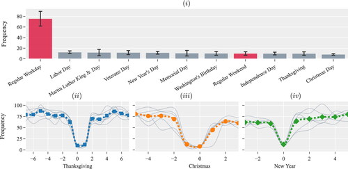
We observe variations in the volume of surgical cases a few business days before and after major holidays. Figure 5(ii)–(iv) present the volume of surgical cases a few business days prior and proceeding to three major holidays. Each of the gray lines represents observations from a particular calendar year. The volume of surgical cases during Thanksgiving, Christmas, and New Year are very low. However, the volume of surgical cases a few days before and after the holidays is typically higher than during regular business days. Such a trend was not observed during other Federal holidays. Thus, we introduce a total of 6 binary features to represent the business days preceding and following Thanksgiving, Christmas, and New Year.

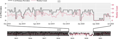
Figure 6(i) presents a snapshot of the volume of cases of the procedure with SID XJS during October 2018 and July 2020 and the number of unique providers scheduled for these procedures by week. We observe that the volume of cases and the number of providers change (increase/decrease) at the same time. A similar trend is observed for the rest of the data (see Figure 6(ii)). In Figure 6(i), the shaded area in this figure captures the impact of the COVID-19 pandemic on the volume of surgical cases. During this period, the weekly volume of cases reduces significantly. To capture the impact of workforce size, represented by the number of providers, on the number of procedures scheduled, we add a feature that represents the total number of unique providers per month.

Figure 6. (i) Snapshot and (ii) timeline show the relationship between the number of primary providers and the number of times procedure XJS was scheduled per week.

Extreme weather conditions like heavy rain and snow could lead to appointment cancelations and traffic accidents. Furthermore, most hospital systems have inclement weather policies in place to provide services during these conditions. In order to evaluate whether weather conditions impact the volume of surgical cases, we conducted the following statistical analysis. We extracted meteorological data from the National Centers for Environmental Information (NCEI) Application Programming Interface (API). We collected this data for the specific meteorological station located near the partnering hospital. Using this data, we determined the snow weekdays during the period of study. Next, we calculated the average and standard deviation of the volume of surgical cases during weekdays without snow and weekdays with snow. We found out that the average volume of surgical cases on weekdays without snow is $\mu$ = 74.21, and the standard deviation is $\sigma$ = 16.38. For snow days, we found $\mu$ = 56.54 and $\sigma$ = 19.81. The difference of these population means is statistically significant at p-value of 0.0093. Thus, to capture the impact of weather conditions on the volume of surgical cases during the period of study, we extracted four features from this meteorological database: (i) the minimum daily temperature, (ii) the maximum daily temperature, (iii) daily precipitation, and (iv) daily snow accumulation depth.

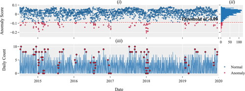
Figure 7(iii) summarizes the total volume of daily records (cases) for the procedure with SID XJS. Figure 7(i) presents the anomaly score for each daily record, and Figure 7(ii) presents the distribution of the anomaly scores. The anomaly score is calculated for each data point using the isolated forest (IsolationForest) algorithm (Ding & Fei, 2013) that is available in the scikit-learn package in Python (Pedregosa et al., 2011). A data point represents the total volume of surgical cases on a particular day. We use the distribution of the anomaly score to determine the anomaly threshold. We select the threshold in such a way that $5\%$ of the data points have a lower anomaly score, and are classified as outliers. We engineer a (binary) feature to represent these outliers.

Figure 7. (i) Anomaly scores per observation of procedure XJS. (ii) Distribution of the anomaly score. (iii) A time series of the procedure with the corresponding anomalies.

2.3. Model development

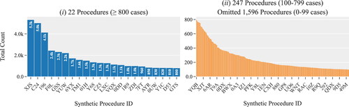
We propose a long short-term memory (LSTM) model to predict the volume of surgical cases per week. LSTM is an artificial recurrent neural network (RNN) architecture capable of learning order dependence in sequential data. Successful implementations of LSTM require large amounts of data. Our data analysis shows that only a few procedures have the necessary data to develop, train and test procedure-specific LSTMs (see Figure 8). For example, for only 22 procedures we have more than 800 records per procedure. These procedures account for 29.5% of the observations. We developed an LSTM model for each of the 22 procedures for which we have sufficient data. The rest of the procedures are clustered together based on certain similarities. An LSTM model is developed for each cluster. We create 26 clusters, which account for 16% of the observations. In the following sections, we provide details of the clustering algorithm and of the LSTM model.

Figure 8. Distribution of surgical procedures based on the total number of observations during the period of study. (i) Procedures with more than 800 observations; and (ii) Procedures with less than 800 observations.

2.3.1. Clustering of surgical procedures

Our data analysis reveals that several procedures belonging to the same service type have a similar description and identification number (proc_id). For example, “surgery on the left hand” and “surgery on the right hand” are two procedures of Orthopedics service type. These two procedures have only minor variations in their description and also share the first digits of their four-digit identification number (proc_id). We have identified nine procedures that share the same first three digits of their proc_id, 133x. These procedures have the word “arthroplasty” in their description. Other common words are “knee,” “hip,” “shoulder,” and “elbow.”

These observations influenced our approach to clustering the less frequently observed procedures. We cluster together procedures that belong to the same service type and have similar descriptions and proc_id. This clustering approach is also motivated by the fact that our forecasts are used to determine the inventory of surgical instruments in the hospital. Surgeries that belong to the same cluster do use similar instruments.

We begin our clustering by creating two lists, a list of words and a list of n-grams commonly used to describe a procedure. The n-grams are sequences of n contiguous words in the description of procedures. For example, suppose the description for an arbitrary procedure is “right index finger amputation”; the bi-grams include “right_index,” “index_finger,” and “finger_amputation.” We clustered those procedures with the common word(s) and/or n-grams in their description and similar ID numbers. This process resulted in the clustering of 230 procedures into 26 clusters.

2.3.2. The long short-term memory model

LSTM is a special kind of recurrent neural network (RNN) that was introduced by Hochreiter and Schmidhuber in 1991 (Hochreiter & Schmidhuber, 1997). An RNN is capable of identifying structures and patterns in the data from earlier stages for the purpose of forecasting future trends via forward and backward propagation. The main challenge with a generic RNN is that does not remember long sequences of data. Different from RNN, LSTM uses gates and a memory line to overcome this challenge. Each LSTM consists of a set of cells where sequences of data are stored. Each cell consists of the Cell State, Hidden State and three types of gates (Forget, Input and Output). Cells act as long-term memory lines along which the information flows. In each cell, the gates regulate the flow of information. The gates determine what data in a sequence is important to keep or discard (Hochreiter & Schmidhuber, 1997).

The proposed model uses the data from the last 4 wk (28 days) to make predictions about the expected volume of surgical cases in next week (7 days). To generate the input for the LSTM model, we divided the dataset into overlapping sequences. As such, only the first and last days of two consecutive sequences are different. Each sequence consists of (historical) data and predictions about next week’s weather. Recall that weather prediction is a feature we have engineered for this LSTM model. Thus, using these sequences as an input for the LSTM model is a challenge. For this reason, we develop an Encoder-Decoder Sequence To Sequence (seq2seq) LSTM model (Sak et al., 2017).

We use the mean squared error (MSE) as the loss function and adaptive moment estimation (Adam) as the optimizer (Kingma & Ba, 2014). We use the Keras deep learning API to build the LSTM model in Python 3.9 (Chollet et al., 2015). Nvidia RTX 3080 GPU is utilized in the training process. The features fed to the LSTM are normalized. We use the value of the coefficient of determination, $R^2,$ the root mean squared error (RMSE) and mean absolute error (MAE) to assess the accuracy of the predicted values. (2) $$R^2=1-\frac{\sum _i{(y_i-{\widehat{y}}_i)}^2}{\sum _i{(y_i-\overline{y})}^2},\mathrm{\hspace{1em}}\mathrm{\hspace{1em}}\mathit{RMSE}=\sqrt{\frac{\sum _i{(y_i-{\widehat{y}}_i)}^2}{n}},\mathrm{\hspace{1em}}\mathrm{\hspace{1em}}\mathit{MAE}=\frac{1}{n}\sum _{i=1}^n\left|y_i-{\widehat{y}}_i\right|,$$(2) where $y_i,$ ${\widehat{y}}_i$ denote the actual and predicted values in day i, respectively. $\overline{y}$ denotes the average value of all observations, and n represents the number of observations in the test dataset.

We perform hyperparameter tuning for every LSTM model developed. We tune five hyperparameters, (i) the number of recurrent layers, (ii) the number of hidden layers, (iii) the dropout probability, (iv) the learning rate, and (v) the number of epochs. We use two approaches for tuning the hyperparameters, a grid search and a Bayesian optimization technique. The grid search evaluates the model for each possible combination of the listed hyperparameters. Each evaluation is performed in isolation. Different from the grid search, the Bayesian optimization technique uses the results from previous evaluations to narrow down the search space. In our experiments, we use Optuna, a Bayesian optimizer of Python (Akiba et al., 2019). We select the hyperparameters that produce the highest RMSE score. The best hyperparameters are exported for the implementation phase or future use.

3. Experimental results and discussions

3.1. Model evaluation

We compare the results of the proposed LSTM model with various popular forecasting models that are available in Python, such as Facebook’s Prophet (Taylor & Letham, 2017), and gradient boosting machine (GBM) (Ke et al., 2017). We use 6 wk of data in our experiments. The results are summarized in Table 1. Based on these results, the proposed LSTM model outperforms both, Prophet and GMB.

Table 1. Performance evaluation.

	LSTM	Facebook Prophet	GBM
R^2	0.875	0.547	0.635
RMSE	1.526	3.548	2.432
MAE	0.882	1.657	1.231

3.2. Experimental results

Figure 9 illustrates the quality of the forecasts for the procedure XJS by the LSTM model. For this procedure, we have a total of 4,742 cases for the period of study. Table 2 provides a summary of different performance measures. These results indicate that the predictions for the next six weeks are of high quality. However, the model’s predictability degrades over time. This observation is supported by the decrease of the value of $R^2,$ the increase of the value of RMSE and MAE (in Table 2), and the increased variance of residuals (in Figure 10) as the prediction interval increases from 6 to 15 wk.

Figure 9. Predictions for procedure XJS.

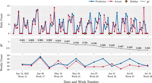
Figure 10. Distribution of the residuals for procedure XJS.

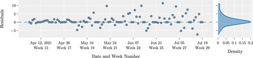
Table 2. Summary of model performance.

	Procedure XJS		Largest cluster: C1
Testing length	6 wk	15 wk	6 wk	15 wk
R^2	0.858	0.341	0.630	0.314
RMSE	1.526	3.091	0.622	0.816
MAE	0.882	1.846	0.429	0.575

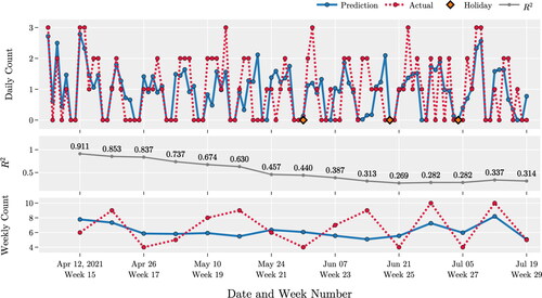
Figure 11 illustrates our forecasts for the largest cluster of surgeries, C1. This cluster consists of seven procedures with a total of 2,307 records. Notice that the procedure XJS has twice the number of observations of this cluster. The number of observations impacts the quality of the forecasting model developed. This explains the difference in the average $R^2$ that we observe for procedure XJS and cluster C1 (see Table 2). The quality of predictions for the 1st week is high for both LSTM models. The corresponding values of $R^2$ are 0.95 and 0.91. However, the values of $R^2$ for predictions beyond 1 week, for cluster C1, drop fast.

Figure 11. Predictions of the largest cluster of procedures, C1.

3.3. Model deployment and monitoring

Figure 12 illustrates the results of the deployment and monitoring process for procedure XJS. The deployment period for this study is from April to October 2021. We trained the model 3 times to predict the daily volume of cases for procedure XJS. After each training of the model, we monitor performance by calculating $R^2.$ The model is retrained when the value of $R^2$ drops below a certain threshold, which for this experiment is set to 0.85. In Figure 12(i), the shaded areas represent outdated predictions. In this figure, we show the prediction and actual values to provide a visual understanding of the changes in the quality of our predictions over time. Figure 12(ii) presents the corresponding values of $R^2.$ The black markers represent the points in time when the model was retrained, and the new predictions replaced the older ones.

Figure 12. Results of model deployment and monitoring for procedure XJS.

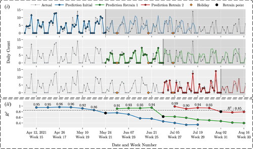
Notice that, the quality of predictions deteriorates faster during the weeks of major Federal holidays. For example, the predictions after the 1st training of the model are highly accurate for 6 wk, from April to the end of May. During this period, there are no Federal holidays. The quality of the forecast deteriorates during the week of Memorial day, which corresponds to the end of this period. After the 2nd training, the quality of prediction is accurate for only 4 wk, after which the quality drops quickly. This period begins with Memorial day and ends with Independence day. After the 3rd training, the quality of predictions is above the threshold level for 4 wk. The quality of predictions remains high because the only Federal holiday observed during this period is Labor day. This observation highlights the impact that fluctuations in the volume of surgical cases during the week of Federal holidays have on the quality of the forecast. These observations justify the use of features we engineered to capture these fluctuations.

3.4. Future research directions

via our numerical analysis, we make observations which are worth further exploration. For example, we notice that the providers’ schedule impacts the volume of surgical cases. Incorporating this schedule in forecasting model via feature engineering could lead to better predictions. We plan to extend our model to consider providers’ schedule.

We did not consider in our analysis the data from 2020 because the daily volume of surgical cases was significantly smaller due to the COVID-19 pandemic. The effects of the pandemic were also observed in 2021. We plan to use the data from 2020 and 2021 to develop forecasting models that capture the impacts of major catastrophic events on predicting the daily volume of surgical cases.

Finally, we will use the results of these predictions to improve the models used by our partnering hospital to predict the inventory of supplies and surgical instruments. We expect that the use of the proposed prediction models will lead to improved inventory management, lower costs, and higher quality of care.

4. Summary and conclusions

The goal of the proposed research is to improve the quality of forecasting the volume of surgical cases at a hospital. Accurate forecasts lead to improved inventory management of supplies and surgical instruments, and in general improved supply chain decisions. These improvements have the potential to reduce the cost of healthcare and improve the quality of care.

We propose a modeling framework which consists of data preprocessing and data exploration, feature engineering, model development, and model deployment and monitoring. The development of this framework is informed by 7 years worth of data from a major hospital in North America. The data exploration identified factors that impacted the volume of surgical cases. Some of these are seasonal factors, such as, certain days of the week, weeks in a year, and months in a year. Other factors are major holidays, the number of providers, and weather conditions. These observations motivated the engineering of a few features which are included in the dataset used for model development. We develop a Long Short-Term Memory (LSTM) Model. LSTM is a special kind of recurrent neural network (RNN), and is capable to identify and remember structures and patterns in the data from earlier stages for the purpose of forecasting future trends. The development of an LSTM model requires large amounts of data. Thus, we could develop an LSTM for each of the 22 procedures that have high volume. These procedures account for 29.5% of the observations. We used a clustering algorithm to group 247 procedures together into 26 clusters. We clustered procedures that belong to the same service type and have similar descriptions. These procedures account for 16% of the observations. We develop an LSTM for each cluster. We tuned the hyperparameters of this model via grid search and Bayesian optimization techniques.

We compare the proposed LSTM with other popular forecasting models, such as, Facebook’s Prophet and the gradient boosting machine. Our analysis demonstrates that the proposed LSTM outperforms these models. We evaluated the performance of our model for procedure XJS and for one of the clusters. These evaluations indicate that the proposed model is of high quality. We deployed the model using data from 2021. The results show that the model should be retrained every 4 wk to provide the best results.

Consent and approval statement

This study has been exempt from the requirement for approval by an institutional review board. We have only used secondary data.

Role of the funders

Not applicable.

Disclosure statement

The authors report there are no competing interests to declare.

Additional information

Funding

The author(s) reported there is no funding associated with the work featured in this article.

Appendix

Table A1. Description of columns in the dataset.

Column Name	Description
date	date of the surgery
proc_id	procedure identification number (i.e., 4 digit numbers)
SID	synthetic procedure identification number (i.e., 3 randomly assigned characters)
proc_descr	procedure description
prov_name	name of the primary healthcare provider

Table A2. Description of features used in the forecasting model.

Feature Name	Type	Description
count^(a)	integer	the number of times a procedure is performed according to the aggregation level (i.e., daily or weekly)
day_of_year, week_of_year	integer	Day of the year and week of the year, respectively
year_XX	binary	Repeated for each year XX. 1 if the date belongs to year XX and 0 when not
sin_YY, cos_YY^(b)	float	Repeated for each YY, where YY comprises of day of the week, month, and quarter. Sine and cosine transformation of feature YY
is_holiday	binary	1 if the date is a Federal holiday and 0 otherwise
is_weekend	binary	1 if the date is either Saturday or Sunday and 0 otherwise
is_anomaly	binary	1 if the date is identified as abnormal and 0 otherwise
num_prov	integer	number of primary providers observed for each month
temp_max, temp_min, prcp, snow_depth	float	Maximum and minimum temperatures, precipitation, snow depth during the entire day, respectively

(a) indicates the target variable.

(b) indicates the encoded cyclical features.

References

- Adams, A., & Vamplew, P. (1998). Encoding and decoding cyclic data. The South Pacific Journal of Natural Science, 16, 54–58.
- Ahmed, N. K., Atiya, A. F., Gayar, N. E., & El-Shishiny, H. (2010). An empirical comparison of machine learning models for time series forecasting. Econometric Reviews, 29(5–6), 594–621. https://doi.org/10.1080/07474938.2010.481556
- Akiba, T., Sano, S., Yanase, T., Ohta, T., & Koyama, M. (2019). Optuna: A next-generation hyperparameter optimization framework.
- Aravazhi, A. (2021). Hybrid machine learning models for forecasting surgical case volumes at a hospital. AI, 2(4), 512–526. https://doi.org/10.3390/ai2040032
- Bam, M., Denton, B. T., Van Oyen, M. P., & Cowen, M. E. (2017). Surgery scheduling with recovery resources. IISE Transactions, 49(10), 942–955. https://doi.org/10.1080/24725854.2017.1325027
- Best, M. J., McFarland, E. G., Anderson, G. F., & Srikumaran, U. (2020). The likely economic impact of fewer elective surgical procedures on us hospitals during the covid-19 pandemic. Surgery, 168(5), 962–967. https://doi.org/10.1016/j.surg.2020.07.014
- Box, G. E., Jenkins, G. M., Reinsel, G. C., & Ljung, G. M. (2015). Time series analysis: Forecasting and control. John Wiley & Sons.
- Boyle, J., Jessup, M., Crilly, J., Green, D., Lind, J., Wallis, M., Miller, P., & Fitzgerald, G. (2012). Predicting emergency department admissions. Emergency Medicine Journal: EMJ, 29(5), 358–365. https://doi.org/10.1136/emj.2010.103531
- Chollet, F., et al. (2015). Keras. https://keras.io
- Cui, Z., Chen, W., & Chen, Y. (2016). Multi-scale convolutional neural networks for time series classification.
- Ding, Z., & Fei, M. (2013). An anomaly detection approach based on isolation forest algorithm for streaming data using sliding window. IFAC Proceedings Volumes, 46(20), 12–17. https://doi.org/10.3182/20130902-3-CN-3020.00044
- Ekström, A., Kurland, L., Farrokhnia, N., Castrén, M., & Nordberg, M. (2015). Forecasting emergency department visits using internet data. Annals of Emergency Medicine, 65(4), 436–442.e1. https://doi.org/10.1016/j.annemergmed.2014.10.008
- Hochreiter, S., & Schmidhuber, J. 11 (1997). Long short-term memory. Neural Computation, 9(8), 1735–1780. ISSN 0899-7667. https://doi.org/10.1162/neco.1997.9.8.1735
- Jones, S. A., Joy, M. P., & Pearson, J. O. N. (2002). Forecasting demand of emergency care. Health Care Management Science, 5(4), 297–305. https://doi.org/10.1023/a:1020390425029
- Kaushik, S., Choudhury, A., Kumar Sheron, P., Dasgupta, N., Natarajan, S., Pickett, L. A., & Dutt, V. (2020). Ai in healthcare: Time-series forecasting using statistical, neural, and ensemble architectures. Frontiers in Big Data, 3(4), 4. https://doi.org/10.3389/fdata.2020.00004
- Ke, G., Meng, Q., Finley, T., Wang, T., Chen, W., Ma, W., Ye, Q., & Liu, T.-Y. (2017). Lightgbm: A highly efficient gradient boosting decision tree. Advances in Neural Information Processing Systems, 30, 3146–3154.
- Kingma, D. P., & Ba, J. (2014). Adam: A method for stochastic optimization. arXiv preprint arXiv:1412.6980.
- Lim, G., & Mobasher, A. (2012). Operating suite nurse scheduling problem: A column generation approachIn Proceedings of the 2012 Industrial and Systems Engineering Research Conference, Orlando, FL,
- Lipton, Z. C., Kale, D. C., Elkan, C., & Wetzel, R., 11 (2015). Learning to diagnose with lstm recurrent neural networks. 4th International Conference on Learning Representations, ICLR 2016 – Conference Track Proceedings https://doi.org/10.48550/arxiv.1511.03677
- Lütkepohl, H., 1 (2006). Chapter 6 forecasting with varma models. Handbook of Economic Forecasting, 1:287–325 ISSN 1574-0706. https://doi.org/10.1016/S1574-0706(05)01006-2
- McCarthy, M. L., Zeger, S. L., Ding, R., Aronsky, D., Hoot, N. R., & Kelen, G. D. (2008). The challenge of predicting demand for emergency department services. Academic Emergency Medicine, 15(4), 337–346. ISSN 1553-2712. https://doi.org/10.1111/J.1553-2712.2008.00083.X
- Muñoz, E., Muñoz, W., III., & Wise, L. (2010). National and surgical health care expenditures, 2005–2025. Annals of Surgery, 251(2), 195–200. https://doi.org/10.1097/SLA.0b013e3181cbcc9a
- Pedregosa, F., Varoquaux, G., Gramfort, A., Michel, V., et al. (2011). Scikit-learn: Machine learning in Python. Journal of Machine Learning Research, 12, 2825–2830.
- Pham, T., Tran, T., Phung, D., & Venkatesh, S. (2016). Deepcare: A deep dynamic memory model for predictive medicine. Lecture Notes in Computer Science (Including Subseries Lecture Notes in Artificial Intelligence and Lecture Notes in Bioinformatics), 9652 LNAI:30–41, 2. ISSN 16113349. https://doi.org/10.1007/978-3-319-31750-2˙3
- Sak, H., Shannon, M., Rao, K., & Beaufays, F. (2017). Recurrent neural aligner: An encoder-decoder neural network model for sequence to sequence mapping. Interspeech, 8, 1298–1302.
- Taylor, S. J., & Letham, B. (2017). Forecasting at scale. PeerJ, 9, 37–45. ISSN 2167-9843. https://doi.org/10.7287/peerj.preprints.3190v2
- Tiwari, V., Furman, W. R., & Sandberg, W. S. (2014). Predicting case volume from the accumulating elective operating room schedule facilitates staffing improvements. Anesthesiology, 121(1), 171–183. https://doi.org/10.1097/ALN.0000000000000287
- UAMS. (2021). Arkansas clinical data repository. https://ar-cdr.uams.edu/.
- Vollmer, M. A., Glampson, B., Mellan, T., Mishra, S., Mercuri, L., Costello, C., Klaber, R., Cooke, G., Flaxman, S., & Bhatt, S. (2021). A unified machine learning approach to time series forecasting applied to demand at emergency departments. BMC Emergency Medicine, 21(1), 1–14. 12 ISSN 1471227X. https://doi.org/10.1186/S12873-020-00395-Y/FIGURES/8
- Widiasari, I. R., Nugroho, L. E., & Widyawan. (2017). Deep learning multilayer perceptron (MLP) for flood prediction model using wireless sensor network based hydrology time series data mining [Paper presentation]. In 2017 International Conference on Innovative and Creative Information Technology (ICITech), 1–5, https://doi.org/10.1109/INNOCIT.2017.8319150
- Zhang, P. G. (2003). Time series forecasting using a hybrid ARIMA and neural network model. Neurocomputing, 50, 159–175. ISSN 0925-2312. https://doi.org/10.1016/S0925-2312(01)00702-0
- Zhao, B., Lu, H., Chen, S., Liu, J., & Wu, D. (2017). Convolutional neural networks for time series classification. Journal of Systems Engineering and Electronics, 28(1), 162–169. https://doi.org/10.21629/JSEE.2017.01.18
- Zheng, A., & Casari, A. (2018). Feature engineering for machine learning: Principles and techniques for data scientists (1st ed.). O’Reilly Media, Inc.
- Zinouri, N., Taaffe, K. M., & Neyens, D. M. (2018). Modelling and forecasting daily surgical case volume using time series analysis. Health Systems (Basingstoke, England), 7(2), 111–119. https://doi.org/10.1080/20476965.2017.1390185